Abstract
Most arsenic cancer risk assessments have been based solely on epidemiological studies to characterize the dose-response relationship for arsenic-associated cancer and to perform risk calculations. However, current epidemiological evidence is too inconsistent and fraught with uncertainty regarding arsenic exposure to provide reliable estimates. This makes it hard to draw a firm conclusion about the shape and slope of the dose-response relationship from individual studies. Meta-analysis is a statistical approach to combining results across studies and offers expanded opportunities for obtaining an improved dose-response relationship. In this study, a meta-analysis of arsenic studies was conducted by combining seven epidemiological studies from different regions to get an overall dose-response relationship between the amount of arsenic intake and the excess probability of bladder cancer. Both the fixed-effect and random-effect models were used to calculate the averaged coefficient of the linear-logistic regression model. A homogeneity test was also conducted. The final product of this research is an aggregated dose-response model in the range of empirical observation of arsenic. Considering the most recent arsenic MCL (maximum contaminant level, i.e. 10μg/L), the associated bladder cancer risk (lifetime excess probability) at this MCL is 2.29 × 10⁻⁵.
Introduction
In risk-based regulation, data are needed to characterize the dose-response relationship for risk calculations. The accuracy of the data and the ability to fit them by an appropriate model in turn determine the scientific validity of a risk assessment [1]. In the case of arsenic risk assessment, there are inadequate data and models from animal experiments, while there are relatively plentiful human data. Therefore, arsenic cancer risk assessments have been mostly based on observational studies in epidemiology [2]. There are many advantages to using epidemiological studies as a source of data for dose-response analysis in risk assessment, including development of direct evidence of carcinogenic or other health effects in humans, thereby avoiding the uncertainty associated with inter-species extrapolation. However, current epidemiological evidence is highly variable and at times conflicting. So it is not appropriate to draw a firm conclusion about the shape or magnitude of the dose-response relationship based on an individual study.
Meta-analysis is a statistical tool for integrating and analyzing data from related but independent studies. Applying a set of statistical procedures, which quantitatively aggregate the results of multiple primary studies, an overall conclusion or summary of average properties such as risk coefficients across these studies may be reached [3]. If conducted appropriately, the overall conclusion or summary measure could be a more objective appraisal of the evidence, and uncertainty and disagreement among studies can also be characterized. Moreover, meta-analysis assists in the exploration and evaluation of results, including reasons for any differences in results between studies. This additional information helps in characterizing uncertainty and locating sources of inter-subject variability [4].
The quantitatively-aggregating ability of meta-analysis allows it to examine relationships not investigated in the original primary studies [3], and to test hypotheses about sources and magnitudes of heterogeneity and bias [5]. Therefore, meta-analysis can be an alternative to a single large, expensive, and logistically problematic study [4]; the use of a single study as the basis for risk assessments; or the use of purely subjective summary judgments in weight-of-evidence determinations. In a word, meta-analysis, if appropriately conducted, is a tool to quantitatively analyze a collection of epidemiological study results, and can be used in risk assessment to combine results across studies with the goal of estimating measures of association with improved precision. In practice, meta-analysis has been used in the steps of hazard identification and dose-response assessment [6].
The objective of this study is to use meta-analysis to combine several epidemiological datasets to produce an aggregated dose-response function for the relationship between bladder cancer risk and arsenic intake from drinking water.
Materials and Methods
Search Methods
The criteria for inclusion of epidemiological studies in the present meta-analysis are: all studies are of a case-control or cohort design, and evaluate the relationship between arsenic concentration in drinking water and bladder cancer; studies are of males, females or of both genders combined; studies examine incidence or mortality as the study outcome; studies provide information required for the statistical analysis; studies are published in English between 1970 and 2005; and studies are referenced in the U.S. EPA IRIS (Integrated Risk Information System), NRC’s (National Research Council) Reports [1, 7] or Medline database. Besides these searches, the list of references in the identified articles was also systematically examined for additional studies.
The study outcomes varied. In cohort studies, relative risks were used as the study outcome; in case-control studies, odds ratios were the outcomes. Considering that bladder cancer is a rare disease, the odds ratio was assumed approximately the same as relative risk, and relative risk was used as the study outcome. Only one cohort mortality study [8] used SMR (standardized mortality rate) as the study outcome. But this study was criticized because “the comparison of the study population to all of Utah is not appropriate for estimating excess risks” and “the study is not powerful enough to estimate excess risks with enough precision to be useful for arsenic risk analysis” [9]. Hence it was excluded in this meta-analysis.
Seven studies were included in the meta-analysis since they satisfied the criteria mentioned above. They were from different regions, including Taiwan, U.S., Argentina, Chile and Finland [10–16]. Most of the study outcomes were adjusted by factors of age, gender and cigarette smoking. The details of these studies are listed in Table 1.

Table 1.
Studies of Bladder Cancer (188)
Rescaling of Exposure
As for deciding the exposure midpoint assigned to a subpopulation, if the highest category of arsenic exposure was open-ended, its interval was set equal to the width between 0 and the lower bound of the open-ended boundary. For example, in the study of Chiou et al. [13], the highest category of arsenic exposure was open-ended (>100); this open-ended interval was setequal to the width between 0 and 100, and its midpoint was 150. If the lowest category was open-ended, the lowest boundary was considered as zero. The upper- and lower-bound values of arsenic concentration in each category were then used to calculate the mid-point of exposure for that subpopulation [17]. Also, the definition of arsenic exposure varied among studies. In most of the articles, “arsenic exposure” means the annual average concentration of arsenic in drinking water (in units of μg/L or ppb). Studies using another exposure index (i.e. lifetime exposure) were rescaled to concentration assuming population-average rates of water ingestion.
Dose-response Model
For each study, using the information on RR (relative risk) and average arsenic exposure (X) for each subpopulation, the hazard as a function of exposure can be modeled as [18] :
Where X is the exposure (in μg/L), ΔX is the difference in arsenic concentration intake between each category of exposure (X) and the reference category in each study (X0). The coefficient b is the fitted slope factor in the linear-logistic regression model. This linear-logistic model estimates the logarithm of the observed relative risks (estimated as the odds ratio in some studies), and accounts for the correlation between risk estimates for separate exposure levels depending on the same reference group.
After finding the coefficient (bi) of each study, the summary estimate is the pooled coefficient (b̄). The individual slopes of each study were combined by weighted average, using the inverse of their variances as weights. The 95% confidence intervals (CI) were calculated for the common regression slopes. The fixed-effects model was first used and the homogeneity test was conducted. The random-effect model was applied when the homogeneity test provided evidence of heterogeneity.
Statistical Methods
The underlying statistical theory of meta-analysis is “Sample Error Theory”. The sample error stems from the variation of characteristics between samples and the original population, given that a sample typically can’t represent the whole population. There are two major sources of variation to be considered when conducting a meta-analysis: (i) within-study variation, resulting from different random sampling errors within each study; and (ii) inter-study variation, resulting from the heterogeneity between studies.
Fixed-effects Model
The fixed-effects model assumes there is only within-study variation in the mean outcomes of a study, and that inter-study variation can be excluded. It also assumes that the underlying population from which studies are generated is the same and has identical characteristics and study effect for all studies considered in the meta-analysis. [19] This is called the homogeneity assumption.
Random-effects Model
The random-effects model assumes both within-study and between-study variations exist. The population from which studies are generated may have different characteristics and study effects. This assumption leads to wider and more conservative confidence intervals than the fixed effects model [19].
Calculating the Summary Estimator
Meta-analysis uses a weighted average of the results from the individual studies:
Where wi is the weight of each study, yi is the parameter being estimated of each study (here, the slope factor), and yw is the weighted average of the parameter being estimated.
The weight usually is the inverse of the variance of the result for each study. The larger studies therefore have more influence than the smaller ones [6, 20]. The weight used for a fixed-effects model generally is:
, and for the random effects model is:
, where si2 is the within-study variation and τi2 is the inter-study variation [19].
Test of Homogeneity
The fixed-effects model assumes that all studies are sampled from the same population, so the k study-specific summary statistics share a common mean θ. A statistical test for the homogeneity of study means is equivalent to testing[19]:
The chi-square test can be employed as a basic statistical test of the homogeneity assumptions [21]:
Where wi (weight) = 1/si2, Ȳ = ∑wiYi/∑wi, and k = number of studies.
If H0 cannot be rejected, we have to accept the null hypotheses; i.e. the k studies share a common mean θ and are homogeneous. Otherwise, if H0 is rejected, it may be concluded that these study means arose from different populations and are not homogeneous. Under this condition, Normand (1999) suggests to “…continue proceeding by either attempting to identify covariates that stratify studies into the homogeneous populations or estimating a random-effects model” [19].
Results
Dose-Response Relationship for Each Study
From Figure 1, we can see that the results of observational studies of arsenic in drinking waster are quite dispersed. In three studies Bates et al. [11], Steinmaus et al. [14], and Bates et al. [16], a dose-response relationship is not evident between the exposure to arsenic and the relative risk of bladder cancer, or is negative. In the study of Kurttio et al. 1999, a much stronger relationship is noted from the limited and lower range of arsenic exposure. Although two studies done by Chiou et al. [10, 13] are different study designs from two different regions in Taiwan, their dose-response relationships are quite similar.
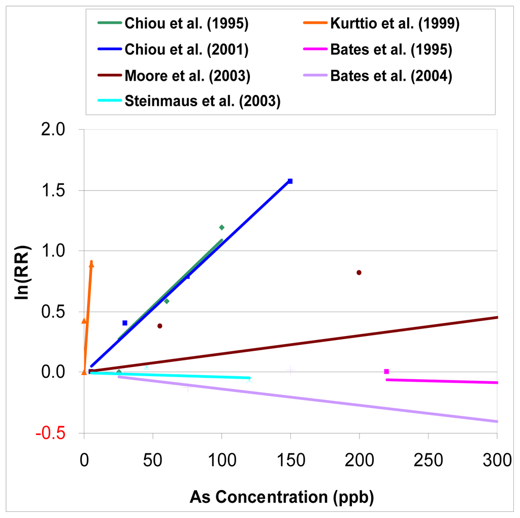
Figure 1.
Dose-response analysis of relative risk of bladder cancer for arsenic intake from drinking water.
Calculating the Summary Estimator and Test of Homogeneity
The fixed-effects model was first used. The pooled estimate of slopes from seven studies was 0.00615 (95% CI: 0.00588, 0.00642), with the unit of lnRR per unit increase of exposure. But the chi-square statistic was quite large (i.e. Q= 3197.110 on 6 degrees of freedom, p= 0.00), which rejects the null hypothesis of homogeneity and means there was evidence of heterogeneity.
The fitted slope (with the unit of lnRR per unit increase of exposure) of each study and the combined estimate of slope by using fixed-effect model are presented as box plots in figure 2. The horizontal line of each study corresponds to its 95% confidence interval, and the size of the square reflects the weight of each study. From Figure 2, it is clear that the Finland study done by Kurttio et al. [12] has a much wider horizontal line and no box, showing that its 95% confidence interval is much wider than other studies but with very little weight. We then concluded that this study might be an outlier for its far lower arsenic exposure. This study was then excluded to solve the problem of heterogeneity. But this didn’t lower the value of the chi-square statistic sufficiently, showing that heterogeneity still exists even in the remaining subset of six studies. Therefore, a random-effect model was used next.
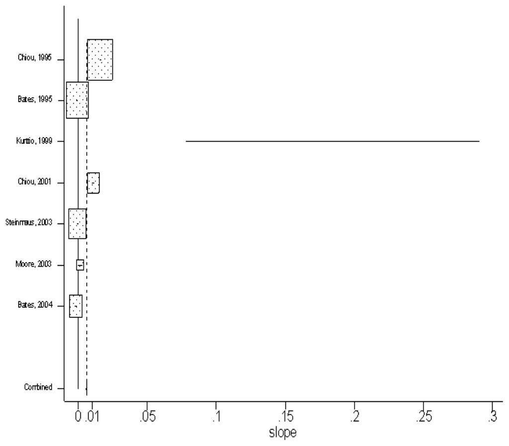
Figure 2.
Slope (with the unit of lnRR per unit increase of exposure) of each study and the combined estimate of slope by using fix-effect model. The horizontal line of each study corresponds to its 95% confidence interval, and the size of the square reflects the weight of each study.
Sensitivity Analysis
To make sure the exclusion of the Finland study done by [12] doesn’t cause a significant effect on the result, another meta-analysis using the random-effect model and including all seven studies was conducted. The average of the slopes is 0.005 (95% C.I.: −0.002, 0.012). Comparing this result with the previous one using the random-effect model but excluding the Finland study, their best-estimates are only slightly different (0.004 vs. 0.005), and the difference between them will be even slighter when exponential functions are applied to these two values. Also, their upper-bound estimates are the same (i.e. 0.012). Therefore, it is appropriate to exclude the Finland study. The comparison of these results is shown in Table 2.

Table 2.
Comparison of the results by using different models and including different studies.
Calculating the Summary Estimator by using the Random-effect model
By using the random-effect model, the pooled estimate of the slopes from the seven studies was found to be 0.004 (in units of per μg/L) (95% CI: −0.03, 0.012). The results are shown in Figure 3.
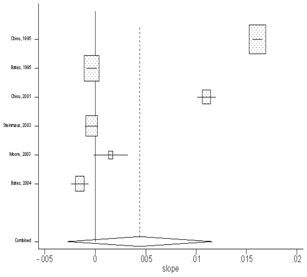
Figure 3.
Slope (with the unit of lnRR per unit increase of exposure) of each study and the combined estimate of slope by using random-effect model.
Figure 4 shows both the summary estimators from the fixed-effect and random-effect models (including six studies).
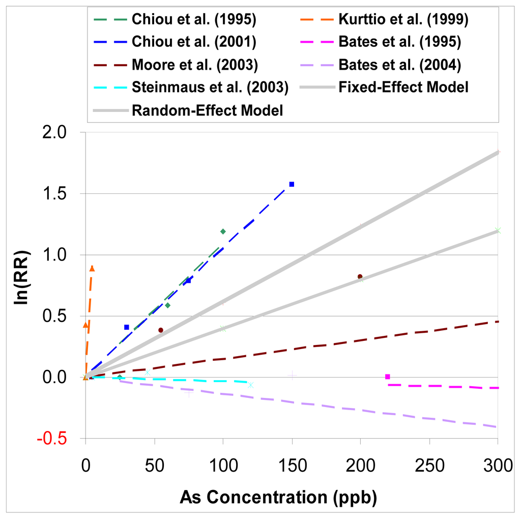
Figure 4.
Dose-response relationship of relative risk of bladder cancer for arsenic intake from drinking water by using fixed-effect and random-effect model.
Risk Calculation
The result of the meta-analysis supports the claim that there is a positive dose-response relationship between exposure to arsenic in drinking water and bladder cancer. Using the results presented above, the best estimate of the relative risk associated with an increase of arsenic exposure can be estimated as:
Were X is the waterborne arsenic concentration in units of μg/L. Using the upper 95% confidence limit, the plausible upper limit of the relative risk associated with an increase of arsenic exposure can be estimated as:
The absolute risk (AR) of bladder cancer is calculated by multiplying the excess relative risk (ERR) by the natural rate (NR) of bladder cancer. Excess relative risk equals the relative risk minus one (i.e. ERR=RR-1). Therefore, AR can be calculated as:
Figure 5 and Table 3 show the results of the AR calculation for bladder cancer associated with a variety of proposed MCLs (maximum contaminant levels) by using two different estimates from the meta-analysis: the best estimate and the upper bound estimate of the slope factor. At the most recent arsenic MCL (i.e. 10 μg/L), the associated bladder cancer risk (lifetime excess probability) is 2.29 × 10⁻⁵ by using the upper bound estimate of the slope factor.
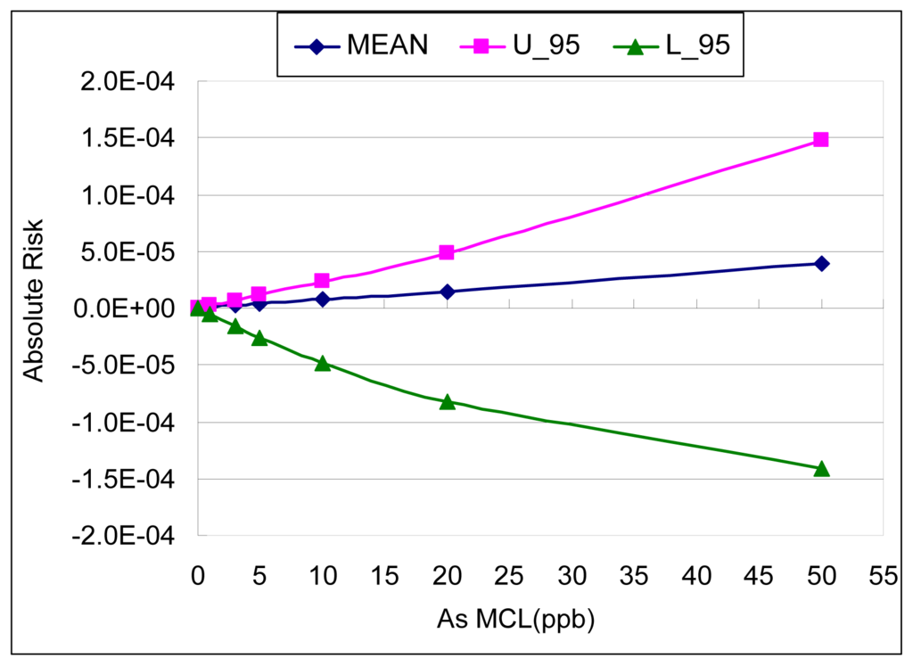
Figure 5.
Absolute Risk of Bladder Cancer at different proposed MCLs (Maximum Contaminant Levels) from meta-analysis. (Mean: the best estimation of slope factor, U_95: the upper bound estimation of slope factor)

Table 3.
Risk of bladder cancer at different MCLs
From the upper bound result of the meta-analysis, the arsenic concentration corresponding to a lifetime excess probability of 10−3 is approximately 160 μg/L; the concentration corresponding to 10−4 is approximately 40 μg/L; and the concentration corresponding to 10−5 is 4.5 μg/L.
Aggregated Slope Factors for Dose-Response Relationship
The slope factor was fitted using the equation of Pc = SF × ADRI, where Pc is the mean probability of cancer, SF is the slope factor, and ADRI is average daily rate of intake of arsenic (μg/kg/day). ADRI (μg/kg/day) was transformed from arsenic MCL (μg/L or ppb) by assuming a tap water ingestion rate of 0.023 L/kg-day. A linear function (characterized by a slope factor) was then fitted as an approximation to the dose-response curve for the meta-analysis results. Figure 6 shows the regression results of slope factors.
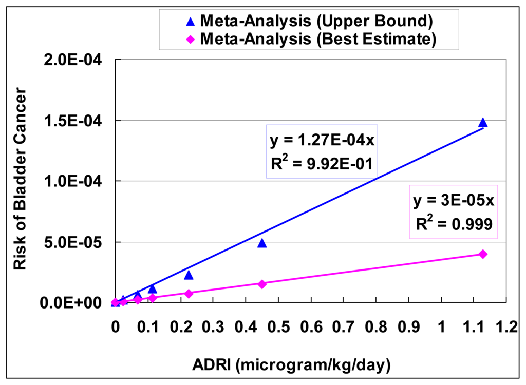
Figure 6.
Slope factors of bladder cancer generated from meta-analysis results.
The best estimate of the slope factor from the meta-analysis is 3.0 × 10⁻⁵ (with unit of probability per μg//kg/day), with the upper bound of 1.27 × 10⁻⁴. These slope factors from the meta-analysis are lower than the ones from the EPA (1.5 × 10⁻³) and NRC (8.85 × 10⁻⁴).
Discussion
In this study, a meta-analysis of arsenic studies was conducted by combining several epidemiological studies from different regions (such as Taiwan, US, Argentina, Chile and Finland) to produce a composite dose-response relationship between the amount of arsenic exposure and the excess probability of cancer. Both the fixed-effect and random-effect models were used to calculate the averaged coefficient of the linear-logistic regression model. A homogeneity test was conducted first to check the heterogeneity among these studies. Because the heterogeneity was found to be high, a random-effect model had to be used. This results in a wider confidence interval of slopes and a more conservative upper bound quantitative summary of risk. The high heterogeneity shows that there are large differences between studies, which suggest it may not be appropriate to simply extrapolate from Taiwanese studies to the U.S.
The final product is an aggregated dose-response model in the range of empirical observation of arsenic. The best estimate of the slope factor from the meta-analysis is 3.0 × 10⁻⁵ (with unit of probability per microgram/kg/day), with the upper bound of 1.27 × 10⁻⁴. These slope factors from the meta-analysis are lower than the ones from the EPA (1.5 × 10⁻³) and NRC (8.85 × 10⁻⁴). There clearly are large differences between the current study and the EPA/NRC results. The possible reason for the difference is because EPA/NRC conducted their study mainly based on data from Taiwan, while we used meta-analysis to combine data from several different regions.
Considering the most recent arsenic MCL (i.e. 10 μg/L), the associated bladder cancer risk (lifetime excess probability) conducted using the upper bound result of the meta-analysis is 2.29 × 10⁻⁵ (7.35 × 10⁻⁶ if the best estimate is used), which is much lower than NRC’s theoretical lifetime excess risk of bladder cancer for U.S. Populations (1.2 × 10⁻³ for female and 2.3 × 10⁻³ for male).
One shortcoming of this study is that there are only seven observational studies available for the meta-analysis. The available data makes it difficult to do further investigation, such as meta-regression to check whether an overall study result varies among subgroups (e.g. study type or location), or a sensitivity analysis to detect the robustness of the findings to different assumptions. New observational studies of arsenic, especially ones involving a case-control or cohort design, need the investment of large amounts of money and time. Even given that requirement, meta-analysis can be an appropriate tool to resolve the discrepancies among existing epidemiological data, and to produce a reasonable generalized dose-response model and its distribution of parameter values.
References
- NRC, Arsenic in Drinking Water; Washington, D.C; National Academy Press, 1999.
- Abernathy, C. O.; Chappell, W. R.; Meek, M. E.; Gibb, H.; Guo, H-R. Is ingested inorganic arsenic a “threshold” carcinogen? Fundamental and Applied Toxicology 1996, 29, 168–175. [Google Scholar]
- Arthur, W.; Bennett, W.; Huffcutt, A. I. Conducting meta-analysis using SAS; N. J. Mahwah; Lawrence Erlbaum Associates, 2001. [Google Scholar]
- Egger, M.; Smith, G. D. Meta-analysis: Potentials and promise. BMJ 1997, 315, 1371–1374. [Google Scholar]
- Greenland, S. Can meta-analysis be salvaged? American Journal of Epidemiology 1994, 140(9), 783–787. [Google Scholar]
- Steenland, K.; Savitz, D. A. Topics in environmental epidemiology; New York; Oxford University Press, 1997. [Google Scholar]
- NRC, Arsenic in Drinking Water. In Update 2001; Washington, D.C; National Academy Press, 2001.
- Lewis, D. R.; Southwick, J. W.; Ouellet-Hellstrom, R.; Rench, J.; Calderon, R. L. Drinking water arsenic in Utah: A cohort mortality study. Environmental Health Perspectives 1999, 107(5), 359–365. [Google Scholar]
- USEPA, 40 CFR Parts 141 and 142, National Primary Drinking Water Regulations; Arsenic and Clarifications to compliance and New Source Contaminants Monitoring; Final Rule; Federal Register. Environmental Protection Agency 2001.
- Chiou, H.; Hsueh, Y.; Liaw, K.; Horng, S.; Chiang, M.; Pu, Y.; Lin, J.; Huang, C.; Chen, C. Incidence of internal cancers and ingested inorganic arsenic: a seven-year follow-up study in Taiwan. Cancer Research 1995, 55(6), 1296–1300. [Google Scholar]
- Bates, M.; Smith, A.; Cantor, K. Case-control study of bladder cancer and arsenic in drinking water. American Journal of Epidemiology 1995, 141(6), 523–530. [Google Scholar]
- Kurttio, P.; Pukkala, E.; Kahelin, H.; Auvinen, A.; Pekkanen, J. Arsenic concentrations in well water and risk of bladder and kidney cancer in Finland. Environmental Health Perspectives 1999, 107(9), 705–710. [Google Scholar]
- Chiou, H.-Y.; Chiou, S.-T.; Hsu, Y.-H.; Chou, Y.-L.; Tseng, C.-H.; Wei, M.-L.; Chen, C.-J. Incidence of transitional cell carcinoma and arsenic in drinking water: A follow-up study of 8,102 residents in an arseniasis-endemic area in Northeastern Taiwan. American Journal of Epidemiology 2001, 153(5), 411–418. [Google Scholar]
- Steinmaus, C.; Yuan, Y.; Bates, M. N.; Smith, A. H. Case-control study of bladder cancer and drinking water arsenic in the western United States. American Journal of Epidemiology 2003, 158(12), 1193–1201. [Google Scholar]
- Moore, L. E.; Smith, A. H.; Eng, C.; DeVries, S.; Kalman, D.; Bhargava, V.; Chew, K.; Ferreccio, C.; Rey, O. A.; Hopenhayn, C.; Biggs, M. L.; Bates, M. N.; Waldman, F. M. P53 alterations in bladder tumors from arsenic and tobacco exposed patients. Carcinogenesis 2003, 24(11), 1785–1791. [Google Scholar]
- Bates, M. N.; Rey, O. A.; Biggs, M. L.; Hopenhayn, C.; Moore, L. E.; Kalman, D.; Steinmaus, C.; Smith, A. H. Case-control study of bladder cancer and exposure to arsenic in Argentina. Am. J. Epidemiol 2004, 159(4), 381–389. [Google Scholar]
- Norat, T.; Lukanova, A.; Ferrari, P.; Riboli, E. Meat consumption and colorectal cancer risk: Dose-response meta-analysis of epidemiological studies. Int. J. of Cancer 2002, 98(2), 241–256. [Google Scholar]
- Greenland, S.; Longnecker, M. Methods for trend estimation from summarized dose-response data, with applications to meta-analysis. American Journal of Epidemiology 1992, 135(11), 1301–1309. [Google Scholar]
- Normand, S.-L. Tutorial in Biostatistics. Meta-analysis: formulating, evaluating, combining, and reporting. Statistics in Medicine 1999, 18, 321–359. [Google Scholar]
- Egger, M.; Smith, G. D.; Phillips, A. N. Meta-analysis: Principles and procedures. BMJ 1997, 315, 1533–1537. [Google Scholar]
- Wang, M. C.; Bushman, B. J. SAS Institute, Integrating results through meta-analytic review using SAS software; Cary, NC; SAS Institute, 1999. [Google Scholar]
© 2006 MDPI. All rights reserved.