
Bayesian Hierarchical Framework from Expert Elicitation in the South African Coal Mining Industry for Compliance Testing


Abstract
1. Introduction
2. Methods
2.1. Study Design and Data Collection
2.2. Expert Elicitation Process
Selection of Experts
2.3. Statistical Methods
2.3.1. Producing Joint Distribution from Experts’ Elicitation
2.3.2. Bayesian Framework
2.3.3. Model Specification Using Current Likelihood Data
2.3.4. Model Specification Using a Non-Informative Prior Distribution, and Informative Prior from the Historical Data and Expert Judgements
2.3.5. The Sensitivity Analysis for the Parameter Space
3. Results
4. Discussion
5. Conclusions
Author Contributions
Funding
Institutional Review Board Statement
Informed Consent Statement
Data Availability Statement
Acknowledgments
Conflicts of Interest
Appendix A

| Category | Description | Statistical Illustration | Exposure Profile | Minimum Frequency |
|---|---|---|---|---|
| 1. | Exposures less than 10% of the OEL 5% of the time | P95 < 0.1% OEL | Very highly controlled | No sampling plan for this category. Measurement results that are below 10% of the OEL will be reported under this category |
| 2. | Exposures exceed 10% of the OEL and less than 50% of the OEL 5% of the time | P95 ≥ 0.1 OEL and <0.5 OEL | Highly controlled | Sample 5% of employees within a HEG on an annual basis with a minimum of 5 samples per HEG, whichever is greater. |
| 3. | Exposures exceed 50% of the OEL and less than OEL 5% of the time | P95 ≥ 0.5 OEL and <OEL | Adequately controlled | Sample 5% of employees within a HEG on a 6-monthly basis with a minimum of 5 samples per HEG, whichever is greater |
| 4. | Exposures exceed the OEL 5% of the time | P95 ≥ OEL | Poorly controlled | Sample 5% of employees within a HEG on a 3-monthly basis with a minimum of 5 samples per HEG, whichever is greater. |
Appendix B. Data Collection Questionnaire
- (a)
- Based on your experience in the industry, what would be your best guess in percentages, of the P95 of exposure concentrations being found in each of the exposure categories?
- (b)
- What would be the maximum and minimum percentages in each of the exposure categories?
- (c)
- How sure are you that the above answers are correct?
Appendix C
| Job Titles | Ratings | SA Exposure Categories, Coal Dust OEL (2 mg/m3) | ||||
|---|---|---|---|---|---|---|
| P95 < 0.1% OEL | P95 ≥ 0.1 OEL and <0.5 OEL | P95≥ 0.5 OEL and <OEL | P95 ≥ OEL | Total (%) | ||
| Job title X (This is an example, say for expert 1) | a | 40% | 5% | 20% | 35% | 100 |
| b | 20% to 70% | 0 to 15% | 2% to 30% | 30 to 90% | ||
| c | 70% sure | 50% sure | 90% sure | 100% sure | ||
| Beltsman | a | 100 | ||||
| b | ||||||
| c | ||||||
| CM Operator | a | 100 | ||||
| b | ||||||
| c | ||||||
| Conveyer belt Attendant | a | 100 | ||||
| b | ||||||
| c | ||||||
| Emico Driver | a | 100 | ||||
| b | ||||||
| c | ||||||
| Electrician | a | 100 | ||||
| b | ||||||
| c | ||||||
| Face Boss | a | 100 | ||||
| b | ||||||
| c | ||||||
| Pump Attendant | a | 100 | ||||
| b | ||||||
| c | ||||||
| Roofbolt Operator | a | 100 | ||||
| b | ||||||
| c | ||||||
| Safety Officer | a | 100 | ||||
| b | ||||||
| c | ||||||
| Shuttle Car Operator | a | 100 | ||||
| b | ||||||
| c | ||||||
References
- U.S. Department of Energy, Energy Information Administration, Office of Coal, Nuclear, Electric and Alternate Fuels. International Energy Outlook. 1991. Available online: http://www.eia.gov/forecasts/ieo/coal.cfm (accessed on 1 October 2022).
- Government Communication and Information System (GCIS): South Africa Yearbook. 2013. Available online: https://www.gcis.gov.za/content/resourcecentre/sa-info/yearbook2013-14 (accessed on 20 April 2022).
- Petsonk, E.L.; Rose, C.; Cohen, R. Coal mine dust lung disease. New lessons from an old exposure. Am. J. Respir. Crit. Care Med. 2013, 1, 1178–1185. [Google Scholar] [CrossRef]
- Soutar, C.; Campbell, S.; Gurr, D.; Lloyd, M.; Love, R.; Cowie, H.; Cowie, A.; Seaton, A. Important deficits of lung function in three modern colliery populations: Relations with dust exposure. Am. Rev. Respir. Dis. 1993, 147, 797–803. [Google Scholar] [CrossRef]
- Attfield, M.D.; Seixas, N.S. Prevalence of pneumoconiosis and its relationship to dust exposure in a cohort of US Bituminous coal miners and ex-miners. Am. J. Ind. Med. 1995, 27, 137–151. [Google Scholar] [CrossRef]
- Made, F.; Kandala, N.B.; Brouwer, D. Compliance Testing and Homogenous Exposure Group Assessment in the South African Coal Mining Industry. Ann. Work Expo. Health 2021, 65, 955–965. [Google Scholar] [CrossRef]
- Gelman, A.; Carlin, J.B.; Stern, H.S.; Dunson, D.B.; Vehtari, A.; Rubin, D.B. Bayesian Data Analysis; CRC Press: Boca Raton, FL, USA, 2013. [Google Scholar]
- Slottje, P.; Van der Sluijs, J.P.; Knol, A.B. Expert Elicitation: Methodological Suggestions for Its Use in Environmental Health Impact Assessments; Utrecht University Repository: Utrecht, The Netherlands, 2008. [Google Scholar]
- U.S. Environmental Protection Agency. Expert Elicitation Task Force White Paper. 2011. Available online: www.epa.gov/stpc/pdfs/eewhite-paper-final.pdf (accessed on 9 January 2022).
- Walker, K.D.; Evans, J.S.; Macintosh, D. Use of expert judgment in exposure assessment. Part I. Characterization of personal exposure to benzene. J. Expo. Sci. Environ. Epidemiol. 2001, 11, 308–322. [Google Scholar] [CrossRef]
- Fischer, H.J.; Vergara, X.P.; Yost, M.; Silva, M.; Lombardi, D.A.; Kheifets, L. Developing a job-exposure matrix with exposure uncertainty from expert elicitation and data modelling. J. Expo. Sci. Environ. Epidemiol. 2017, 27, 7–15. [Google Scholar] [CrossRef]
- Knol, A.B.; de Hartog, J.J.; Boogaard, H.; Slottje, P.; van der Sluijs, J.P.; Lebret, E.; Cassee, F.R.; Wardekker, J.A.; Ayres, J.G.; Borm, P.J. Brunekreef, Expert elicitation on ultrafine particles: Likelihood of health effects and causal pathways. Part. Fibre Toxicol. 2009, 6, 19. [Google Scholar] [CrossRef]
- Hoek, G.; Boogaard, H.; Knol, A.; De Hartog, J.; Slottje, P.; Ayres, J.G.; Borm, P.; Brunekreef, B.; Donaldson, K.; Forastiere, F.; et al. Concentration-response functions for ultrafine particles and all-cause mortality and hospital admissions: Results of a European expert panel elicitation. Environ. Sci. Technol. 2010, 44, 476–482. [Google Scholar] [CrossRef]
- Ramachandran, G.; Banerjee, S.; Vincent, J. Expert judgment and occupational hygiene: Application to aerosol speciation in the nickel primary production industry. Ann. Occup. Hyg. 2003, 47, 461–475. [Google Scholar]
- Hewett, P.; Logan, P.; Mulhausen, J.; Ramachandran, G.; Banerjee, S. Rating exposure control using Bayesian decision analysis. J. Occup. Environ. Hyg. 2006, 3, 568–581. [Google Scholar] [CrossRef]
- NIOSH. Particulates not otherwise regulated, total: Method 0500. In NIOSH Manual of Analytical Methods, 4th ed.; DHHS (NIOSH) Publication No. 94-113; United States Department of Health and Human Services, Centers for Disease Control and Prevention: Cincinnati, OH, USA, 1994. Available online: www.cdc.gov/niosh/nmam/ (accessed on 20 August 2022).
- Hemming, V.; Burgman, M.A.; Hanea, A.M.; McBride, M.F.; Wintle, B.C. A practical guide to structured expert elicitation using the IDEA protocol. Methods Ecol. Evol. 2018, 9, 169–180. [Google Scholar] [CrossRef]
- Adams-Hosking, C.; McBride, M.F.; Baxter, G.; Burgman, M.; De Villiers, D.; Kavanagh, R.; Lawler, I.; Lunney, D.; Melzer, A.; Menkhorst, P.; et al. Use of expert knowledge to elicit population trends for the koala (Phascolarctos cinereus). Divers. Distrib. 2016, 22, 249–262. [Google Scholar] [CrossRef]
- Hanea, A.M.; McBride, M.F.; Burgman, M.A.; Wintle, B.C. Classical meets modern in the IDEA protocol for structured expert judgement. J. Risk Res. 2018, 21, 417–433. [Google Scholar] [CrossRef]
- Bedford, T.; Cooke, R.M. Mathematical Tools for Probabilistic Risk Analysis; Cambridge University Press: Cambridge, UK, 2001. [Google Scholar]
- Hanea, A.M.; Wilkinson, D.P.; McBride, M.P.; Lyon, A.; van Ravenzwaaij, D.; Singleton, T.F.; Gray, C.; Mandel, D.R.; Willcox, A.; Gould, E.; et al. Mathematically aggregating experts’ predictions of possible futures. PLoS ONE 2021, 16, e0256919. [Google Scholar] [CrossRef]
- Cooke, R.M.; Probst, K.N. Highlights of the Expert Judgment Policy Symposium and Technical Workshop. Conference Summary. 2006. Available online: http://www.rff.org/expertjudgementdocuments/documents/workshopdocs/RFFConf_06-ExpertJudgment.pdf (accessed on 20 July 2022).
- StataCorp. Stata Statistical Software: Release 14; StataCorp LP: College Station, TX, USA, 2015. [Google Scholar]
- Stan Development Team. RStan: The R Interface to Stan. R Package Version 2.18.2. 2018. Available online: http://mc-stan.org (accessed on 19 March 2022).
- Makowski, D.; Ben-Shachar, M.S.; Lüdecke, D. bayestestR: Describing effects and their uncertainty, existence and significance within the Bayesian framework. J. Open Source Softw. 2019, 4, 1541. [Google Scholar] [CrossRef]
- R Core Team. R: A Language and Environment for Statistical Computing; R Foundation for Statistical Computing: Vienna, Austria, 2015; Available online: https://www.r-project.org/ (accessed on 10 April 2021).
- Oakley, J.E.; O’Hagan, A. SHELF: The Sheffield Elicitation Framework (Version 4); School of Mathematics and Statistics, University of Sheffield: Sheffield, UK, 2019. [Google Scholar]
- Barlow, R.E.; Mensing, R.W.; Smiriga, N.G. Combination of Experts’ Opinions Based on Decision Theory. In Reliability and Quality Control; Basu, A.P., Ed.; Elsevier Science Publishers (North-Holland): New York, NY, USA, 1986; pp. 9–19. [Google Scholar]
- Garthwaite, P.H.; Kadane, J.B.; O’Hagan, A. Statistical methods for eliciting probability distributions. J. Am. Stat. Assoc. 2005, 100, 680–701. [Google Scholar] [CrossRef]
- Carlin, B.P.; Louis, T.A. Bayesian Methods for Data Analysis, 3rd ed.; Chapman & Hall/CRC: Boca Raton, FL, USA, 2008. [Google Scholar]
- Quick, H.; Huynh, T.; Ramachandran, G. A method for constructing informative priors for Bayesian modelling of occupational hygiene data. Ann. Work Expo. Health 2017, 61, 67–75. [Google Scholar]
- Baldos, U.L.C.; Viens, F.G.; Hertel, T.W.; Fuglie, K.O. R&D spending, knowledge capital, and agricultural productivity growth: A Bayesian approach. Am. J. Agric. Econ. 2019, 101, 291–310. [Google Scholar]
- Made, F.; Kandala, N.B.; Brouwer, D. Bayesian hierarchical modelling of historical data of the South African coal mining industry for compliance testing. Int. J. Environ. Res. Public Health 2022, 19, 4442. [Google Scholar] [CrossRef]
- Gelfand, A.E.; Smith, A.F.M. Sampling-based approaches for calculating marginal densities. J. Am. Stat. Assoc. 1990, 85, 398–409. [Google Scholar] [CrossRef]
- BS EN 689:2018; Workplace Exposure—Measurement of Exposure by Inhalation to Chemical Agents—Strategy for Testing Compliance with Occupational Exposure Limit Values. British Standards Institution: Brussels, Belgium, 2018.
- Ignacio, J.; Bullock, B. (Eds.) A Strategy for Assessing and Managing Occupational Exposures, 3rd ed.; AIHA Press: Fairfax, VA, USA, 2006. [Google Scholar]
- Banerjee, S.; Ramachandran, G.; Vadali, M.; Sahmel, J. Bayesian hierarchical framework for occupational hygiene decision making. Ann. Occup. Hyg. 2014, 58, 1079–1093. [Google Scholar]
- Logan, P.W.; Ramachandran, G.; Mulhausen, J.R.; Hewett, P. Occupational exposure decisions: Can limited data interpretation training help improve accuracy? Ann. Occup. Hyg. 2009, 53, 311–324. [Google Scholar]
- Vadali, M.; Ramachandran, G.; Banerjee, S. Effect of training, education, professional experience and need for cognition on decision making in occupational exposure assessment. Ann. Occup. Hyg. 2012, 56, 292–304. [Google Scholar]
- Joint ACGIH-AIHA Task Group on Occupational Exposure Databases. Data elements for occupational exposure databases: Guidelines and recommendations for airborne hazards and noise. Appl. Occup. Environ. Hyg. 1996, 11, 1294–1313. [Google Scholar] [CrossRef]
- Rajan, B.; Alesbury, B.; Carton, C.; Gérin, M.; Litske, H.; Marquart, H.; Olsen, E.; Scheffers, T.; Stamm, R.; Woldbaek, T. European proposal for core information for the storage and exchange of workplace exposure measurements on chemical agents. Appl. Occup. Environ. Hyg. 1997, 12, 31–37. [Google Scholar] [CrossRef]
- Kahneman, D.; Slovic, P.; Tversky, A. Judgment under Uncertainty: Heuristics and Biases; Cambridge University Press: Cambridge, UK, 1982. [Google Scholar]
- Gilovich, T.; Griffin, D.; Kahneman, D. Heuristics and Biases: The Psychology of Intuitive Judgment; Cambridge University Press: Cambridge, UK, 2002. [Google Scholar]

| Data | Year | n | AM | SD | GM | GSD | p-Value * |
|---|---|---|---|---|---|---|---|
| Current data | |||||||
| Beltsman | 2015 | 18 | 0.76 | 0.72 | 0.48 | 2.94 | 0.5694 |
| CM Operator | 2018 | 116 | 2.08 | 1.87 | 1.28 | 3.30 | 0.1014 |
| Conveyer belt Attendant | 2015 | 29 | 0.93 | 0.75 | 0.66 | 2.41 | 0.0917 |
| Emico Driver | 2015 | 24 | 1.13 | 1.02 | 0.54 | 5.11 | 0.3116 |
| Electrician | 2015 | 52 | 1.55 | 1.52 | 0.87 | 3.75 | 0.0617 |
| Face Boss | 2018 | 35 | 1.56 | 1.76 | 0.80 | 3.68 | 0.8640 |
| Pump Attendant | 2016 | 18 | 0.74 | 0.82 | 0.41 | 3.41 | 0.3955 |
| Roofbolt Operator | 2018 | 101 | 1.77 | 1.66 | 1.11 | 3.03 | 0.0853 |
| Safety Officer | 2018 | 16 | 2.78 | 2.05 | 2.06 | 2.45 | 0.8169 |
| Shuttle Car Operator | 2018 | 46 | 1.60 | 1.34 | 1.08 | 2.62 | 0.1615 |
| Historical data | |||||||
| Beltsman | 2009 | 14 | 1.07 | 0.89 | 0.66 | 3.31 | 0.1653 |
| CM Operator | 2009 | 11 | 2.10 | 2.05 | 0.70 | 8.46 | 0.1573 |
| Conveyer belt Attendant | 2009 | 7 | 0.64 | 0.56 | 0.42 | 2.92 | 0.3012 |
| Emico Driver | 2009 | 6 | 0.81 | 0.73 | 0.43 | 4.29 | 0.5319 |
| Electrician | 2009 | 14 | 1.70 | 2.03 | 0.75 | 5.31 | 0.3618 |
| Face Boss | 2009 | 22 | 1.00 | 0.97 | 0.46 | 4.89 | 0.8495 |
| Pump Attendant | 2009 | 8 | 0.66 | 0.69 | 0.42 | 2.86 | 0.3679 |
| Roofbolt Operator | 2009 | 8 | 1.70 | 2.58 | 0.81 | 3.54 | 0.5319 |
| Safety Officer | 2009 | 8 | 0.70 | 0.56 | 0.38 | 4.57 | 0.4060 |
| Shuttle Car Operator | 2016 | 10 | 1.3 | 1.11 | 0.69 | 4.59 | 0.2352 |
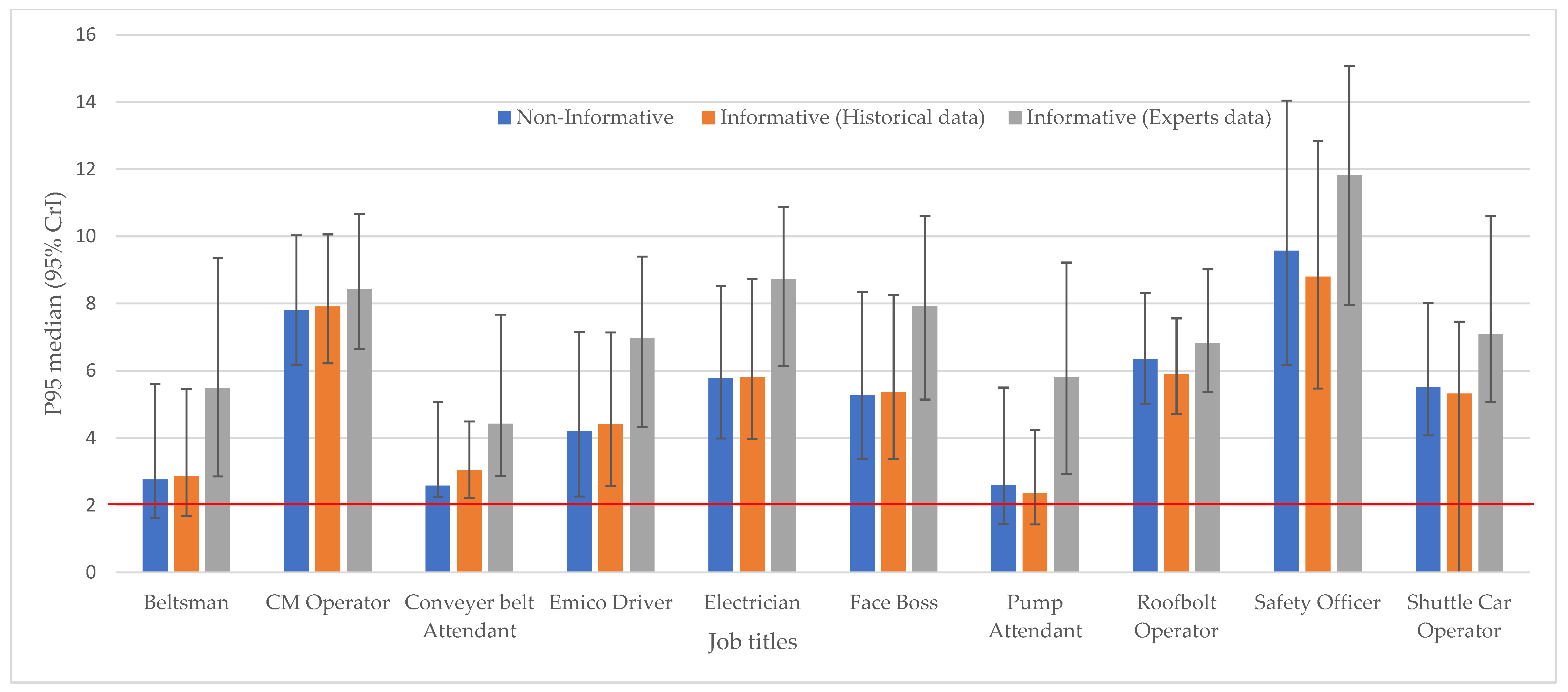
| Non-Informative | Informative from Historical Data | Informative from Expert Judgments | |||||||
|---|---|---|---|---|---|---|---|---|---|
| Job Titles | GM | GSD | P95 | GM | GSD | P95 | GM | GSD | P95 |
| Median (95% CrI) | Median (95% CrI) | Median (95% CrI) | Median (95% CrI) | Median (95% CrI) | Median (95% CrI) | Median (95% CrI) | Median (95% CrI) | Median (95% CrI) | |
| Beltsman | 0.48 (0.28, 0.83) | 2.90 (2.48, 3.64) | 2.77 (1.63, 5.60) | 0.47 (0.27, 0.80) | 3.01 (2.61, 3.66) | 2.87 (1.67, 5.46) | 0.84 (0.50, 1.38) | 3.10 (2.67, 3.58) | 5.48 (2.86, 9.36) |
| CM Operator | 1.28 (1.03, 1.59) | 2.99 (2.80, 3.23) | 7.80 (6.18, 10.03) | 1.25 (1.00, 1.57) | 3.06 (2.87, 3.29) | 7.91 (6.22, 10.06) | 1.37 (1.11, 1.70) | 3.00 (2.82, 3.22) | 8.42 (6.65, 10.66) |
| Conveyer belt Attendant | 0.66 (0.48, 0.94) | 2.59 (2.32, 3.03) | 2.59 (2.25, 5.06) | 0.64 (0.47, 0.87) | 2.57 (2.33, 2.95) | 3.04 (2.21, 4.50) | 0.80 (0.55, 1.21) | 2.84 (2.53, 3.30) | 4.43 (2.88, 7.67) |
| Emico Driver | 0.51 (0.26, 0.90) | 3.58 (3.09, 4.24) | 4.21 (2.26, 7.15) | 0.56 (0.34, 0.92) | 3.47 (3.03, 4.02) | 4.41 (2.58, 7.14) | 0.91 (0.58, 1.33) | 3.41 (3.08, 3.79) | 6.98 (4.33, 9.40) |
| Electrician | 0.86 (0.60, 1.22) | 3.18 (2.87, 3.57) | 5.78 (3.99, 8.52) | 0.83 (0.57, 1.18) | 3.26 (2.96, 3.64) | 5.82 (3.97, 8.43) | 1.31 (0.98, 1.69) | 3.14 (2.89, 3.39) | 8.72 (6.14, 10.87) |
| Face Boss | 0.79 (0.51, 1.20) | 3.16 (2.80, 3.64) | 5.27 (3.38, 8.34) | 0.75 (0.47, 1.16) | 3.28 (2.92, 3.74) | 5.35 (3.38, 8.25) | 1.19 (0.83, 1.64) | 3.13 (2.83, 3.45) | 7.92 (5.14, 10.61) |
| Pump Attendant | 0.40 (0.22, 0.74) | 3.11 (2.63, 3.91) | 2.61 (1.44, 5.50) | 0.38 (0.24, 0.62) | 2.99 (2.60, 3.65) | 2.35 (1.43, 4.25) | 0.82 (0.48, 1.32) | 3.24 (2.80, 3.70) | 5.80 (2.94, 9.22) |
| Roofbolt Operator | 1.11 (0.90, 1.39) | 2.88 (2.69, 3.12) | 6.34 (5.02, 8.31) | 1.04 (0.84, 1.29) | 2.86 (2.68, 3.10) | 5.90 (4.72, 7.56) | 1.17 (0.94, 1.47) | 2.91 (2.73, 3.16) | 6.82 (5.36, 9.02) |
| Safety Officer | 1.98 (1.24, 2.93) | 2.59 (2.27, 3.06) | 9.57 (6.17, 14.04) | 1.57 (0.88, 2.44) | 2.84 (2.50,3.36) | 8.80 (5.47, 12.83) | 2.30 (1.54, 3.18) | 2.68 (2.42, 3.00) | 11.81 (7.96, 15.07) |
| Shuttle Car Operator | 1.08 (0.81, 1.45) | 2.69 (2.46, 3.04) | 5.52 (4.08, 8.01) | 1.05 (0.80, 1.38) | 2.68 (0.80, 1.38) | 5.32 (3.98, 7.46) | 1.35 (1.03, 1.84) | 2.73 (2.50, 3.06) | 7.10 (5.06, 10.60) |
| HEG | Non-Informative | Informative from Historical Data | Informative from Experts’ Data | ||||||||||||
|---|---|---|---|---|---|---|---|---|---|---|---|---|---|---|---|
| P95 | Category 1 | Category 2 | Category 3 | Category 4 | P95 | Category 1 | Category 2 | Category 3 | Category 4 | P95 | Category 1 | Category 2 | Category 3 | Category 4 | |
| Beltsman | 2.77 | 0 | 0.25% | 12.07% | 87.67% | 2.87 | 0 | 0.18% | 9.52% | 90.29% | 5.48 | 0 | 0 | 0.06% | 99.95% |
| CM Operator | 7.80 | 0 | 0 | 0 | 100% | 7.91 | 0 | 0 | 0 | 100% | 8.42 | 0 | 0 | 0 | 100% |
| Conveyer belt Attendant | 2.59 | 0 | 0 | 0.38% | 99.62% | 3.04 | 0 | 0 | 0.40% | 99.60% | 4.43 | 0 | 0 | 0.02% | 99.99% |
| Emico Driver | 4.21 | 0 | 0.03% | 1.04% | 98.93% | 4.41 | 0 | 0 | 0.19% | 99.81% | 6.98 | 0 | 0 | 0 | 100% |
| Electrician | 5.78 | 0 | 0 | 0 | 100% | 5.82 | 0 | 0 | 0 | 100% | 8.72 | 0 | 0 | 0 | 100% |
| Face Boss | 5.27 | 0 | 0 | 0 | 100% | 5.35 | 0 | 0 | 0 | 100% | 7.92 | 0 | 0 | 0 | 100% |
| Pump Attendant | 2.61 | 0 | 1.16% | 19.14% | 79.69% | 2.35 | 0 | 0.91% | 25.99% | 73.09% | 5.80 | 0 | 0 | 0.06% | 99.94% |
| Roofbolt Operator | 6.34 | 0 | 0 | 0 | 100% | 5.90 | 0 | 0 | 0 | 100% | 6.82 | 0 | 0 | 0 | 100% |
| Safety Officer | 9.57 | 0 | 0 | 0 | 100% | 8.80 | 0 | 0 | 0 | 100% | 11.81 | 0 | 0 | 0 | 100% |
| Shuttle Car Operator | 5.52 | 0 | 0 | 0 | 100% | 5.32 | 0 | 0 | 0 | 100% | 7.10 | 0 | 0 | 0 | 100% |
| Grouping | Using Parameter Values from BDA | Placing No Restrictions on Bounds | Using Different Parameter Values | ||||||||||
|---|---|---|---|---|---|---|---|---|---|---|---|---|---|
| Category 1 | Category 2 | Category 3 | Category 4 | Category 1 | Category 2 | Category 3 | Category 4 | Category 1 | Category 2 | Category 3 | Category 4 | ||
| Pump Attendant | Non-informative | 0 | 1.16% | 19.14% | 79.69% | 0 | 0 | 0 | 100% | 0 | 1.24% | 20.85 | 77.91% |
| Historical data | 0 | 0.91% | 25.99% | 73.09% | 0 | 0 | 0 | 100% | 0 | 1.62% | 29.11% | 69.27% | |
| Exert judgments | 0 | 0 | 0.06% | 99.94% | 0 | 0 | 0 | 100% | 0 | 0 | 0.09% | 99.91% | |
| Shuttle Car Operator | Non-informative | 0 | 0 | 0 | 100% | 0 | 0 | 0 | 100% | 0 | 0 | 0 | 100% |
| Historical data | 0 | 0 | 0 | 100% | 0 | 0 | 0 | 100% | 0 | 0 | 0 | 100% | |
| Exert judgments | 0 | 0 | 0 | 100% | 0 | 0 | 0 | 100% | 0 | 0 | 0 | 100% | |
Disclaimer/Publisher’s Note: The statements, opinions and data contained in all publications are solely those of the individual author(s) and contributor(s) and not of MDPI and/or the editor(s). MDPI and/or the editor(s) disclaim responsibility for any injury to people or property resulting from any ideas, methods, instructions or products referred to in the content. |
© 2023 by the authors. Licensee MDPI, Basel, Switzerland. This article is an open access article distributed under the terms and conditions of the Creative Commons Attribution (CC BY) license (https://creativecommons.org/licenses/by/4.0/).
Share and Cite
Made, F.; Kandala, N.-B.; Brouwer, D. Bayesian Hierarchical Framework from Expert Elicitation in the South African Coal Mining Industry for Compliance Testing. Int. J. Environ. Res. Public Health 2023, 20, 2496. https://doi.org/10.3390/ijerph20032496
Made F, Kandala N-B, Brouwer D. Bayesian Hierarchical Framework from Expert Elicitation in the South African Coal Mining Industry for Compliance Testing. International Journal of Environmental Research and Public Health. 2023; 20(3):2496. https://doi.org/10.3390/ijerph20032496
Chicago/Turabian StyleMade, Felix, Ngianga-Bakwin Kandala, and Derk Brouwer. 2023. "Bayesian Hierarchical Framework from Expert Elicitation in the South African Coal Mining Industry for Compliance Testing" International Journal of Environmental Research and Public Health 20, no. 3: 2496. https://doi.org/10.3390/ijerph20032496
APA StyleMade, F., Kandala, N.-B., & Brouwer, D. (2023). Bayesian Hierarchical Framework from Expert Elicitation in the South African Coal Mining Industry for Compliance Testing. International Journal of Environmental Research and Public Health, 20(3), 2496. https://doi.org/10.3390/ijerph20032496