
Linking the Urban Environment and Health: An Innovative Methodology for Measuring Individual-Level Environmental Exposures

 , ,
, ,
Abstract
1. Introduction
2. Materials and Methods
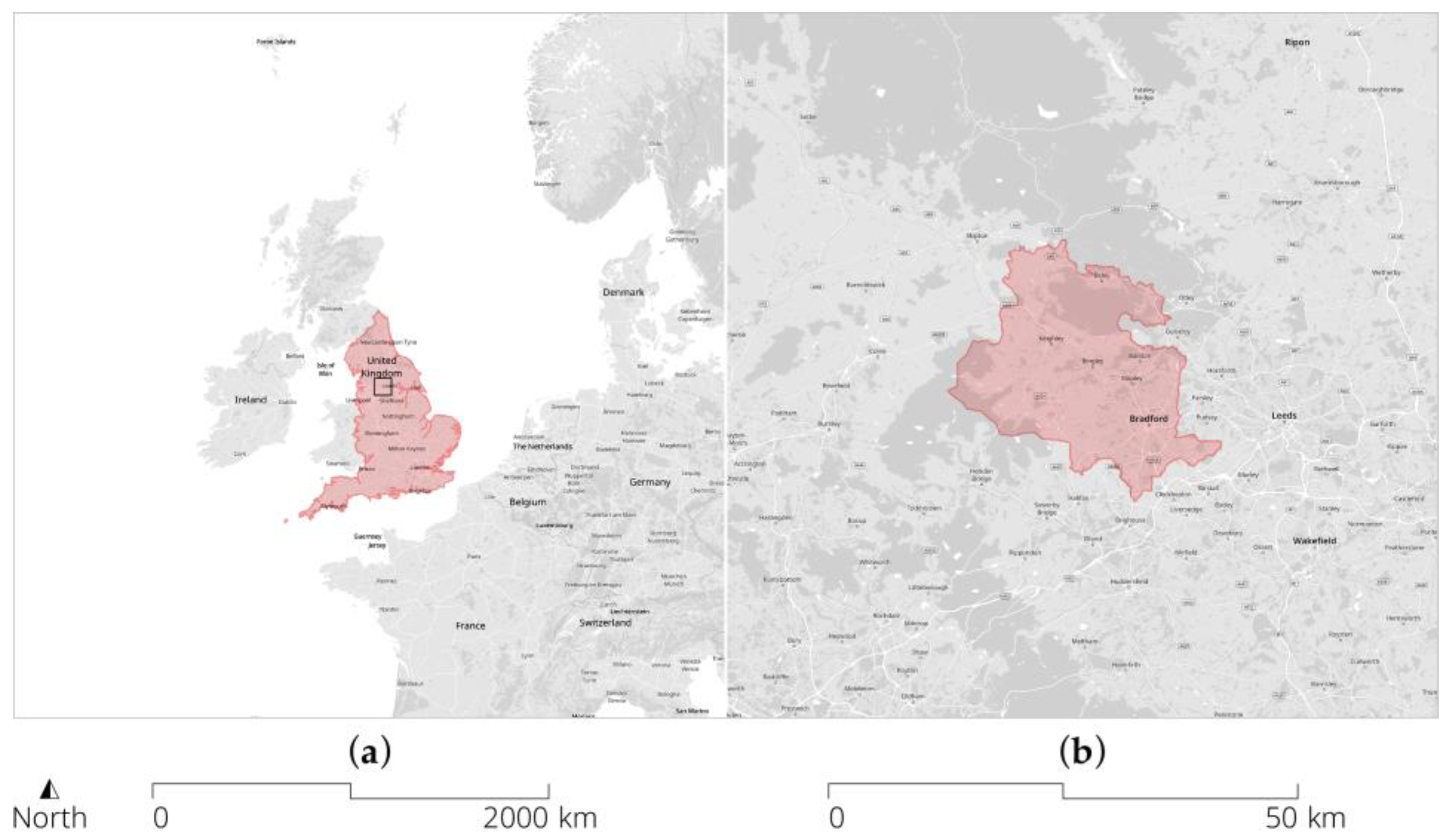
2.1. Setting
2.2. Data Linkage
2.3. Built Environmental Data Sources
2.4. Construction of Exposure Variables
2.5. Selection of Environmental Domains
2.5.1. Air Quality
2.5.2. Road Traffic
2.5.3. Greenness and Greenspace
2.5.4. Public Transport
2.5.5. Walkability and Land-Use Intensity
2.5.6. Street Centrality
2.5.7. Built Form
2.5.8. Indoor Qualities
2.5.9. Food Environments
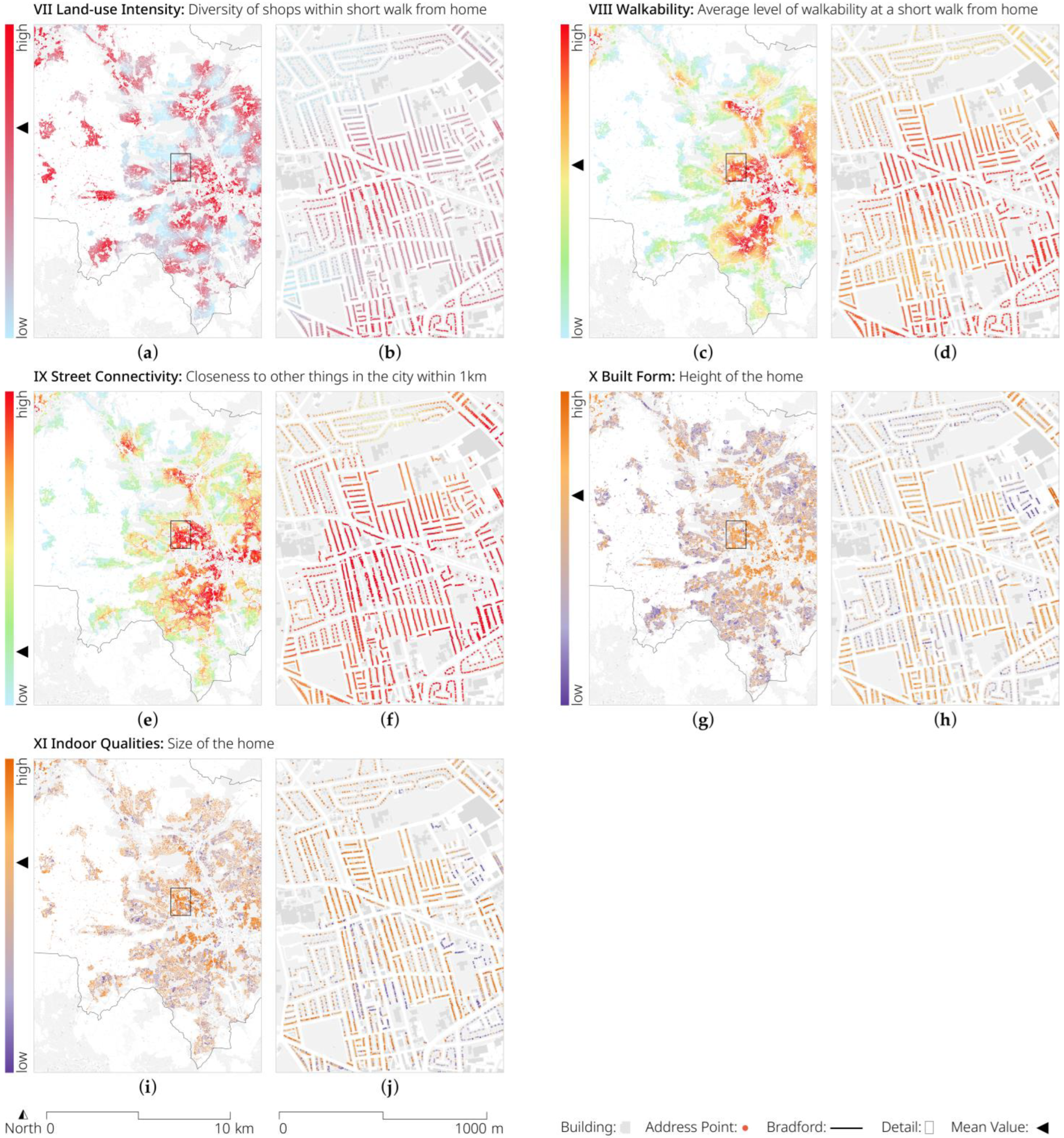
3. Results: Built Environment Indicators
4. Discussion
5. Conclusions
Author Contributions
Funding
Institutional Review Board Statement
Informed Consent Statement
Data Availability Statement
Acknowledgments
Conflicts of Interest
References
- World Health Organization. Setting Global Research Priorities for Urban Health; World Health Organization: Geneva, Switzerland, 2022; ISBN 978-92-4-004182-0. [Google Scholar]
- Brunekreef, B.; Holgate, S.T. Air Pollution and Health. Lancet 2002, 360, 1233–1242. [Google Scholar] [CrossRef] [PubMed]
- Kampa, M.; Castanas, E. Human Health Effects of Air Pollution. Environ. Pollut. 2008, 151, 362–367. [Google Scholar] [CrossRef] [PubMed]
- Mannucci, P.M.; Harari, S.; Martinelli, I.; Franchini, M. Effects on Health of Air Pollution: A Narrative Review. Intern. Emerg. Med. 2015, 10, 657–662. [Google Scholar] [CrossRef]
- Basner, M.; Babisch, W.; Davis, A.; Brink, M.; Clark, C.; Janssen, S.; Stansfeld, S. Auditory and Non-Auditory Effects of Noise on Health. Lancet 2014, 383, 1325–1332. [Google Scholar] [CrossRef] [PubMed]
- Gupta, A.; Gupta, A.; Jain, K.; Gupta, S. Noise Pollution and Impact on Children Health. Indian J. Pediatr. 2018, 85, 300–306. [Google Scholar] [CrossRef] [PubMed]
- Passchier-Vermeer, W.; Passchier, W.F. Noise Exposure and Public Health. Environ. Health Perspect. 2000, 108, 123–131. [Google Scholar] [CrossRef]
- Gianfredi, V.; Buffoli, M.; Rebecchi, A.; Croci, R.; Oradini-Alacreu, A.; Stirparo, G.; Marino, A.; Odone, A.; Capolongo, S.; Signorelli, C. Association between Urban Greenspace and Health: A Systematic Review of Literature. Int. J. Environ. Res. Public Health 2021, 18, 5137. [Google Scholar] [CrossRef]
- Kondo, M.; Fluehr, J.; McKeon, T.; Branas, C. Urban Green Space and Its Impact on Human Health. Int. J. Environ. Res. Public Health 2018, 15, 445. [Google Scholar] [CrossRef]
- Twohig-Bennett, C.; Jones, A. The Health Benefits of the Great Outdoors: A Systematic Review and Meta-Analysis of Greenspace Exposure and Health Outcomes. Environ. Res. 2018, 166, 628–637. [Google Scholar] [CrossRef]
- Fong, K.C.; Hart, J.E.; James, P. A Review of Epidemiologic Studies on Greenness and Health: Updated Literature through 2017. Curr. Environ. Health Rep. 2018, 5, 77–87. [Google Scholar] [CrossRef]
- Gubbels, J.S.; Kremers, S.P.J.; Droomers, M.; Hoefnagels, C.; Stronks, K.; Hosman, C.; de Vries, S. The Impact of Greenery on Physical Activity and Mental Health of Adolescent and Adult Residents of Deprived Neighborhoods: A Longitudinal Study. Health Place 2016, 40, 153–160. [Google Scholar] [CrossRef] [PubMed]
- James, P.; Banay, R.F.; Hart, J.E.; Laden, F. A Review of the Health Benefits of Greenness. Curr. Epidemiol. Rep. 2015, 2, 131–142. [Google Scholar] [CrossRef] [PubMed]
- Flint, E.; Cummins, S.; Sacker, A. Associations between Active Commuting, Body Fat, and Body Mass Index: Population Based, Cross Sectional Study in the United Kingdom. BMJ 2014, 349, g4887. [Google Scholar] [CrossRef] [PubMed]
- Rojas-Rueda, D.; de Nazelle, A.; Teixidó, O.; Nieuwenhuijsen, M.J. Health Impact Assessment of Increasing Public Transport and Cycling Use in Barcelona: A Morbidity and Burden of Disease Approach. Prev. Med. 2013, 57, 573–579. [Google Scholar] [CrossRef]
- Koohsari, M.J.; Kaczynski, A.T.; Mcormack, G.R.; Sugiyama, T. Using Space Syntax to Assess the Built Environment for Physical Activity: Applications to Research on Parks and Public Open Spaces. Leis. Sci. 2014, 36, 206–216. [Google Scholar] [CrossRef]
- Nichani, V.; Koohsari, M.J.; Oka, K.; Nakaya, T.; Shibata, A.; Ishii, K.; Yasunaga, A.; Vena, J.E.; McCormack, G.R. Associations between Neighbourhood Street Connectivity and Sedentary Behaviours in Canadian Adults: Findings from Alberta’s Tomorrow Project. PLoS ONE 2022, 17, e0269829. [Google Scholar] [CrossRef]
- Lai, K.Y.; Kumari, S.; Gallacher, J.; Webster, C.; Sarkar, C. Associations of Residential Walkability and Greenness with Arterial Stiffness in the UK Biobank. Environ. Int. 2022, 158, 106960. [Google Scholar] [CrossRef]
- Hamano, T.; Li, X.; Sundquist, J.; Sundquist, K. Association between Childhood Obesity and Neighbourhood Accessibility to Fast-Food Outlets: A Nationwide 6-Year Follow-Up Study of 944,487 Children. Obes. Facts 2017, 10, 559–568. [Google Scholar] [CrossRef]
- Libuy, N.; Church, D.; Ploubidis, G.B.; Fitzsimons, E. Fast Food and Childhood Obesity: Evidence from Great Britain; CLS: London, UK, 2022. [Google Scholar]
- Patterson, R.; Risby, A.; Chan, M.Y. Consumption of Takeaway and Fast Food in a Deprived Inner London Borough: Are They Associated with Childhood Obesity? BMJ Open 2012, 2, e000402. [Google Scholar] [CrossRef]
- Capasso, L.; D’Alessandro, D. Housing and Health: Here We Go Again. Int. J. Environ. Res. Public Health 2021, 18, 12060. [Google Scholar] [CrossRef]
- Amerio, A.; Brambilla, A.; Morganti, A.; Aguglia, A.; Bianchi, D.; Santi, F.; Costantini, L.; Odone, A.; Costanza, A.; Signorelli, C.; et al. COVID-19 Lockdown: Housing Built Environment’s Effects on Mental Health. Int. J. Environ. Res. Public Health 2020, 17, 5973. [Google Scholar] [CrossRef] [PubMed]
- McCormack, G.R.; Koohsari, M.J.; Turley, L.; Nakaya, T.; Shibata, A.; Ishii, K.; Yasunaga, A.; Oka, K. Evidence for Urban Design and Public Health Policy and Practice: Space Syntax Metrics and Neighborhood Walking. Health Place 2021, 67, 102277. [Google Scholar] [CrossRef] [PubMed]
- Christiansen, L.B.; Cerin, E.; Badland, H.; Kerr, J.; Davey, R.; Troelsen, J.; van Dyck, D.; Mitáš, J.; Schofield, G.; Sugiyama, T.; et al. International Comparisons of the Associations between Objective Measures of the Built Environment and Transport-Related Walking and Cycling: IPEN Adult Study. J. Transp. Health 2016, 3, 467–478. [Google Scholar] [CrossRef] [PubMed]
- Berke, E.M.; Koepsell, T.D.; Moudon, A.V.; Hoskins, R.E.; Larson, E.B. Association of the Built Environment with Physical Activity and Obesity in Older Persons. Am. J. Public Health 2007, 97, 486–492. [Google Scholar] [CrossRef] [PubMed]
- Frank, L.D.; Sallis, J.F.; Conway, T.L.; Chapman, J.E.; Saelens, B.E.; Bachman, W. Many Pathways from Land Use to Health: Associations between Neighborhood Walkability and Active Transportation, Body Mass Index, and Air Quality. J. Am. Plan. Assoc. 2006, 72, 75–87. [Google Scholar] [CrossRef]
- Renalds, A.; Smith, T.H.; Hale, P.J. A Systematic Review of Built Environment and Health. Fam. Community Health 2010, 33, 68–78. [Google Scholar] [CrossRef] [PubMed]
- Zhang, X.; Melbourne, S.; Sarkar, C.; Chiaradia, A.; Webster, C. Effects of Green Space on Walking: Does Size, Shape and Density Matter? Urban Stud. 2020, 57, 3402–3420. [Google Scholar] [CrossRef]
- Brook, J.R.; Setton, E.M.; Seed, E.; Shooshtari, M.; Doiron, D.; Awadalla, P.; Brauer, M.; Hu, H.; McGrail, K.; Stieb, D.; et al. The Canadian Urban Environmental Health Research Consortium—A Protocol for Building a National Environmental Exposure Data Platform for Integrated Analyses of Urban Form and Health. BMC Public Health 2018, 18, 114. [Google Scholar] [CrossRef]
- Ali, M.U.; Rashid, A.; Yousaf, B.; Kamal, A. Health Outcomes of Road-Traffic Pollution among Exposed Roadside Workers in Rawalpindi City, Pakistan. Hum. Ecol. Risk Assess. Int. J. 2017, 23, 1330–1339. [Google Scholar] [CrossRef]
- Liu, S.; Guo, J.; Chen, H. Analysis of Pollutant Exposure of Pedestrian in Urban Street. J. Transp. Syst. Eng. Inf. Technol. 2011, 11, 180–185. [Google Scholar] [CrossRef]
- Papadogeorgou, G.; Kioumourtzoglou, M.-A.; Braun, D.; Zanobetti, A. Low Levels of Air Pollution and Health: Effect Estimates, Methodological Challenges, and Future Directions. Curr. Environ. Health Rep. 2019, 6, 105–115. [Google Scholar] [CrossRef] [PubMed]
- Zhao, L.; Wang, X.; He, Q.; Wang, H.; Sheng, G.; Chan, L.Y.; Fu, J.; Blake, D.R. Exposure to Hazardous Volatile Organic Compounds, PM10 and CO While Walking along Streets in Urban Guangzhou, China. Atmos. Environ. 2004, 38, 6177–6184. [Google Scholar] [CrossRef]
- Zhou, Y.; Levy, J. The Impact of Urban Street Canyons on Population Exposure to Traffic-Related Primary Pollutants. Atmos. Environ. 2008, 42, 3087–3098. [Google Scholar] [CrossRef]
- Ortegon-Sanchez, A.; McEachan, R.R.C.; Albert, A.; Cartwright, C.; Christie, N.; Dhanani, A.; Islam, S.; Ucci, M.; Vaughan, L. Measuring the Built Environment in Studies of Child Health—A Meta-Narrative Review of Associations. Int. J. Environ. Res. Public Health 2021, 18, 10741. [Google Scholar] [CrossRef] [PubMed]
- Jia, P.; Luo, M.; Li, Y.; Zheng, J.; Xiao, Q.; Luo, J. Fast-food Restaurant, Unhealthy Eating, and Childhood Obesity: A Systematic Review and Meta-analysis. Obes. Rev. 2021, 22, 12944. [Google Scholar] [CrossRef] [PubMed]
- Kelly, B.D.; O’Callaghan, E.; Waddington, J.L.; Feeney, L.; Browne, S.; Scully, P.J.; Clarke, M.; Quinn, J.F.; McTigue, O.; Morgan, M.G.; et al. Schizophrenia and the City: A Review of Literature and Prospective Study of Psychosis and Urbanicity in Ireland. Schizophr. Res. 2010, 116, 75–89. [Google Scholar] [CrossRef] [PubMed]
- Lai, K.Y.; Sarkar, C.; Kumari, S.; Ni, M.Y.; Gallacher, J.; Webster, C. Calculating a National Anomie Density Ratio: Measuring the Patterns of Loneliness and Social Isolation across the UK’s Residential Density Gradient Using Results from the UK Biobank Study. Landsc. Urban Plan. 2021, 215, 104194. [Google Scholar] [CrossRef]
- Giles-Corti, B.; Vernez-Moudon, A.; Reis, R.; Turrell, G.; Dannenberg, A.L.; Badland, H.; Foster, S.; Lowe, M.; Sallis, J.F.; Stevenson, M.; et al. City Planning and Population Health: A Global Challenge. Lancet 2016, 388, 2912–2924. [Google Scholar] [CrossRef]
- Sallis, J.F.; Glanz, K. The Role of Built Environments in Physical Activity, Eating, and Obesity in Childhood. Future Child. 2006, 16, 89–108. [Google Scholar] [CrossRef]
- Pont, M.B.; Marcus, L. Innovations in Measuring Density: From Area and Location Density to Accessible and Perceived Density; TU Delft: Delft, The Netherlands, 2014; p. 26. [Google Scholar]
- Hillier, B. Space Is the Machine: A Configurational Theory of Architecture; Cambridge University Press: Cambridge, UK, 1996; ISBN 978-0-9556224-0-3. [Google Scholar]
- Cyril, S.; Oldroyd, J.C.; Renzaho, A. Urbanisation, Urbanicity, and Health: A Systematic Review of the Reliability and Validity of Urbanicity Scales. BMC Public Health 2013, 13, 513. [Google Scholar] [CrossRef]
- Howell, N.A.; Booth, G.L. The Weight of Place: Built Environment Correlates of Obesity and Diabetes. Endocr. Rev. 2022, 43, bnac005. [Google Scholar] [CrossRef] [PubMed]
- Lee, C.; Moudon, A.V. Physical Activity and Environment Research in the Health Field: Implications for Urban and Transportation Planning Practice and Research. J. Plan. Lit. 2004, 19, 147–181. [Google Scholar] [CrossRef]
- Haynes, R.; Daras, K.; Reading, R.; Jones, A. Modifiable Neighbourhood Units, Zone Design and Residents’ Perceptions. Health Place 2007, 13, 812–825. [Google Scholar] [CrossRef]
- Smith, G.; Gidlow, C.; Davey, R.; Foster, C. What Is My Walking Neighbourhood? A Pilot Study of English Adults’ Definitions of Their Local Walking Neighbourhoods. Int. J. Behav. Nutr. Phys. Act. 2010, 7, 34. [Google Scholar] [CrossRef]
- Charreire, H.; Feuillet, T.; Roda, C.; Mackenbach, J.D.; Compernolle, S.; Glonti, K.; Bárdos, H.; Le Vaillant, M.; Rutter, H.; Mckee, M.; et al. Self-Defined Residential Neighbourhoods: Size Variations and Correlates across Five European Urban Regions. Obes. Rev. 2016, 17, 9–18. [Google Scholar] [CrossRef]
- Fishbein, M.; Ajzen, I. Predicting and Changing Behavior; Psychology Press: New York, NY, USA, 2011; ISBN 978-0-8058-5924-9. [Google Scholar]
- Wright, J.; Small, N.; Raynor, P.; Tuffnell, D.; Bhopal, R.; Cameron, N.; Fairley, L.; Lawlor, D.A.; Parslow, R.; Petherick, E.S.; et al. Cohort Profile: The Born in Bradford Multi-Ethnic Family Cohort Study. Int. J. Epidemiol. 2013, 42, 978–991. [Google Scholar] [CrossRef] [PubMed]
- Office for National Statistics (ONS). Population and Household Estimates, England and Wales: Census 2021, Unrounded Data. Available online: https://www.ons.gov.uk/peoplepopulationandcommunity/populationandmigration/populationestimates/bulletins/populationandhouseholdestimatesenglandandwales/census2021unroundeddata#cite-this-statistical-bulletin (accessed on 1 December 2022).
- Ministry of Housing, Communities & Local Government. In The English Indices of Deprivation 2019; Statistical Release: London, UK, 2019; p. 31.
- City of Bradford Metropolitan District Council. Population Report 2021 Census; Intelligence Bulletin; City of Bradford Metropolitan District Council: Bradford, UK, 2022; p. 4. [Google Scholar]
- Office for National Statistics (ONS). National Life Tables—Life Expectancy in the UK: 2018 to 2020; Statistical Bulletin; Office for National Statistics: London, UK, 2021. [Google Scholar]
- Sohal, K.; Mason, D.; Birkinshaw, J.; West, J.; McEachan, R.; Elshehaly, M.; Cooper, D.; Shore, R.; McCooe, M.; Lawton, T.; et al. Connected Bradford: A Whole System Data Linkage Accelerator. Wellcome Open Res. 2022, 7, 26. [Google Scholar] [CrossRef]
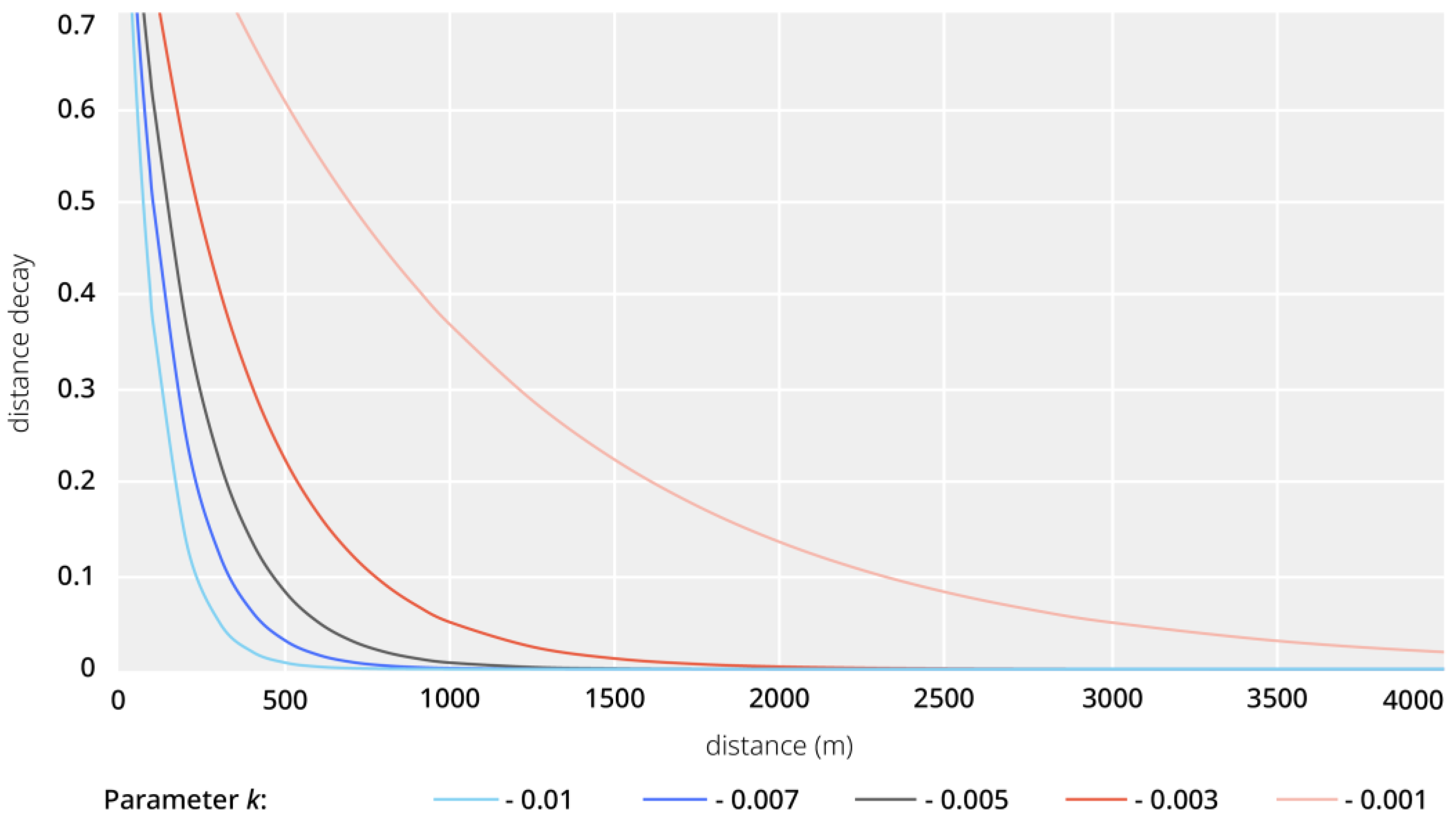
- Vale, D.S.; Pereira, M. The Influence of the Impedance Function on Gravity-Based Pedestrian Accessibility Measures: A Comparative Analysis. Environ. Plan. B Urban Anal. City Sci. 2017, 44, 740–763. [Google Scholar] [CrossRef]
- Konstantinoudis, G.; Padellini, T.; Bennett, J.; Davies, B.; Ezzati, M.; Blangiardo, M. Long-Term Exposure to Air-Pollution and COVID-19 Mortality in England: A Hierarchical Spatial Analysis. Environ. Int. 2021, 146, 106316. [Google Scholar] [CrossRef]
- Villeneuve, P.J.; Goldberg, M.S. Methodological Considerations for Epidemiological Studies of Air Pollution and the SARS and COVID-19 Coronavirus Outbreaks. Environ. Health Perspect. 2020, 128, 095001. [Google Scholar] [CrossRef]
- City of Bradford Metropolitan District Council. 2021–2022 Air Quality Annual Status Report (ASR); City of Bradford Metropolitan District Council: Bradford, UK, 2022; p. 221. [Google Scholar]
- Hegewald, J.; Schubert, M.; Freiberg, A.; Romero Starke, K.; Augustin, F.; Riedel-Heller, S.G.; Zeeb, H.; Seidler, A. Traffic Noise and Mental Health: A Systematic Review and Meta-Analysis. Int. J. Environ. Res. Public Health 2020, 17, 6175. [Google Scholar] [CrossRef] [PubMed]
- McEachan, R.R.C.; Yang, T.C.; Roberts, H.; Pickett, K.E.; Arseneau-Powell, D.; Gidlow, C.J.; Wright, J.; Nieuwenhuijsen, M. Availability, Use of, and Satisfaction with Green Space, and Children’s Mental Wellbeing at Age 4 Years in a Multicultural, Deprived, Urban Area: Results from the Born in Bradford Cohort Study. Lancet Planet. Health 2018, 2, e244–e254. [Google Scholar] [CrossRef] [PubMed]
- Natural England. ‘Nature Nearby’: Accessible Natural Greenspace Guidance; Natural England: York, UK, 2010; pp. 1–98. [Google Scholar]
- WHO Regional Office for Europe. Urban Green Spaces and Health: A Review of Evidence; WHO Regional Office for Europe: Copenhagen, Denmark, 2016; p. 92. [Google Scholar]
- Dhanani, A.; Tarkhanyan, L.; Vaughan, L. Estimating Pedestrian Demand for Active Transport Evaluation and Planning. Transp. Res. Part A Policy Pract. 2017, 103, 54–69. [Google Scholar] [CrossRef]
- Hillier, B.; Hanson, J. The Social Logic of Space; Cambridge University Press: Cambridge, UK, 1984; ISBN 978-0-521-23365-1. [Google Scholar]
- Hillier, B. Spatial Configuration and Use Density at the Urban Level: Towards a Predictive Model, Final Report to the Science and Engineering Research Council; Unit for Architectural Studies, Bartlett School of Architecture and Planning, University College London: London, UK, 1986. [Google Scholar]
- Turner, A. Angular Analysis. In Proceedings of the Third International Space Syntax Symposium, Atlanta, GA, USA, 7–11 May 2001; pp. 1–11. [Google Scholar]
- Hillier, B.; Iida, S. Network and Psychological Effects in Urban Movement. In Spatial Information Theory Lecture Notes in Computer Science 3603; Cohn, A., Mark, D., Eds.; Springer: Berlin/Heidelberg, Germany, 2005; pp. 475–490. [Google Scholar]
- Sharmin, S.; Kamruzzaman, M. Meta-Analysis of the Relationships between Space Syntax Measures and Pedestrian Movement. Transp. Rev. 2018, 38, 524–550. [Google Scholar] [CrossRef]
- Berghauser Pont, M.; Haupt, P. The Spacemate: Density and the Typomorphology of the Urban Fabric. In Urbanism Laboratory for Cities and Regions: Progress of Research Issues in Urbanism; van der Hoeven, F.D., Rosemann, H.J., Eds.; IOS Press: Delft, The Netherlands, 2007; pp. 10–28. [Google Scholar]
- Kickert, C.C.; Pont, M.B.; Nefs, M. Surveying Density, Urban Characteristics, and Development Capacity of Station Areas in the Delta Metropolis. Environ. Plan. B Plan. Des. 2014, 41, 69–92. [Google Scholar] [CrossRef]
- World Health Organization. WHO Global Air Quality Guidelines. Particulate Matter (PM2.5 and PM10), Ozone, Nitrogen Dioxide, Sulfur Dioxide and Carbon Monoxide; World Health Organization: Geneva, Switzerland, 2021. [Google Scholar]
- Krenz, K.; McEachan, R.; Subiza-Pérez, M.; Watmuff, A.; Yang, T.; Vaughan, L. Exploring Relationships between Exposure to Fast Food Outlets and Childhood Obesity at Differing Spatial Resolutions: Results from the Born in Bradford Cohort Study. Lancet 2022, 400, S55. [Google Scholar] [CrossRef]
- Green, M.A.; Hobbs, M.; Ding, D.; Widener, M.; Murray, J.; Reece, L.; Singleton, A. The Association between Fast Food Outlets and Overweight in Adolescents Is Confounded by Neighbourhood Deprivation: A Longitudinal Analysis of the Millennium Cohort Study. Int. J. Environ. Res. Public Health 2021, 18, 13212. [Google Scholar] [CrossRef]


| No. | Environmental Domain | Exposure Measurement | Spatial Relationship | Distance Type and Radii | Data Source |
|---|---|---|---|---|---|
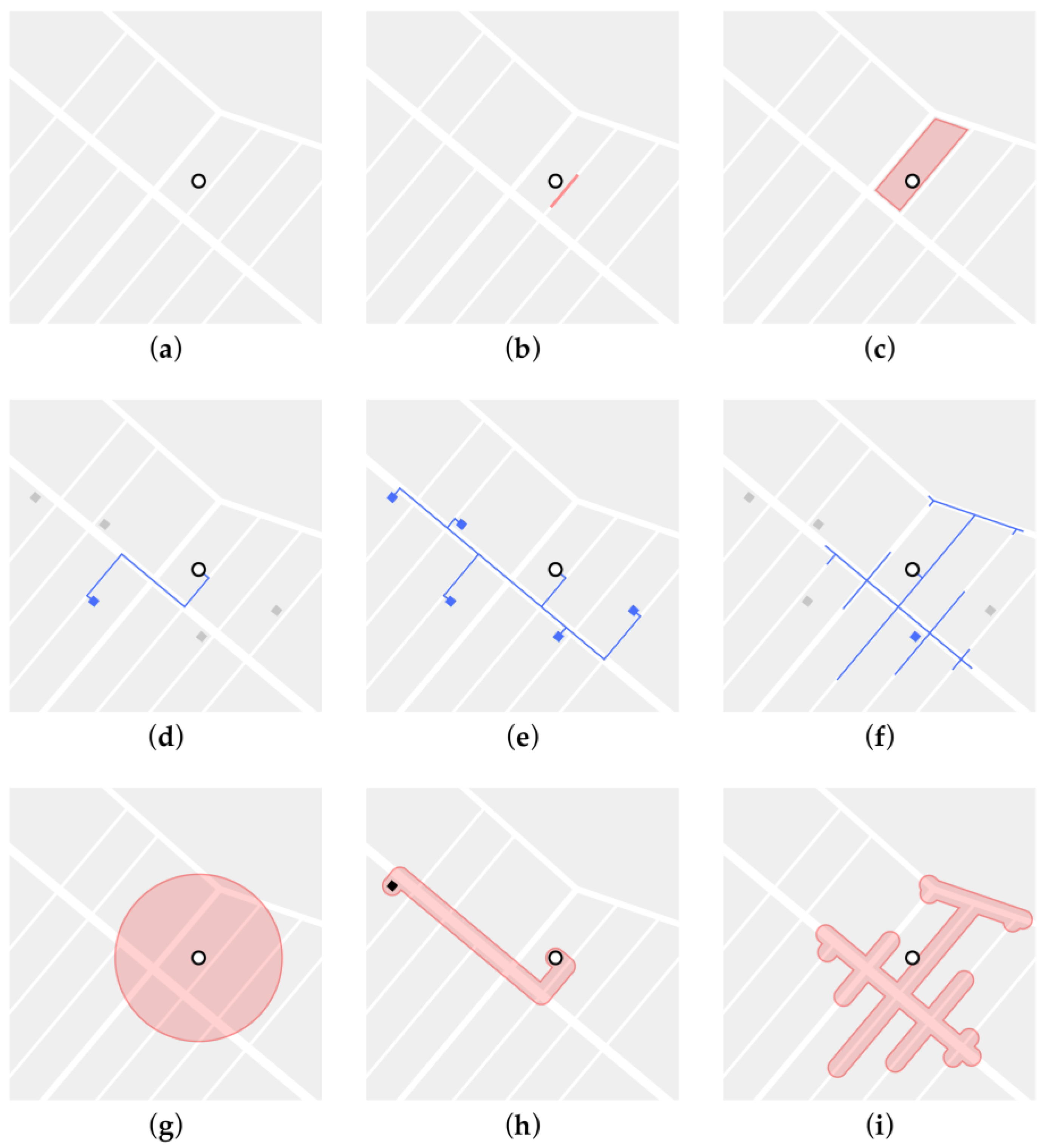
| I | Air Quality | Concentration of Particulate Matter (PM) 10, PM 2.5, and nitrogen oxides (NOx) | (g), (i) | (1), 100, 300, 500, 1000, 1500 | Environmental modelling, City of Bradford, Defra |
| II | Road Traffic | Average traffic volume and level of congestion | (b), (f) | (2), 100, 300 | Basemap Journey Time data |
| III | Greenness | Normalised Difference Vegetation Index (NDVI) | (b), (i) | (1), 100, 300, 500, 1000, 1500 | NASA Landsat 8–9 |
| IV | Greenspace | Accessibility of green spaces entrance points by class (e.g., play space, public park or garden, and religious grounds) | (d), (e), (f) | (2), (4), 300, 500, 1000, 2000, 5000 | OS Open Greenspace |
| V | Public Transport | Accessibility of public transport stops by class (e.g., bus, metro, rail, and coach) | (d), (e), (f) | (2), (4), 300, 500, 1000, 2000, 5000 | NaPTAN |
| VI | Food Environment | Accessibility of all food outlets, fast-food outlets, and ratio of fast-food outlets | (d), (e), (f), (h) | (2), (4), 300, 500, 1000, 2000, 5000 | POI |
| VII | Land-use Intensity | Shannon’s Diversity Index (SDI) | (g), (i) | (1), 100, 300, 500, 1000, 1500 | POI |
| VIII | Walkability | Walkability Index (WI) | (g), (i) | (1), 100, 300, 500, 1000, 1500 | NaPTAN, POI, UK Census, OS Highways, and OS AddressBase |
| IX | Street Centrality | Betweenness and closeness centrality | (b), (f) | (2), 300, 500, 1000, 15,000, 2000 | OS Highways |
| X | Built Form | Building footprint, building height, building volume, building floor area, floor space index (FSI), ground space index (GSI), open-space ratio (OSR), average building layers of floors (L), build form, construction age band, number of storeys, dwelling type, and tenure type | (a), (c) | - | OS MasterMap, OS Highways, and EPC |
| XI | Indoor Qualities | Energy consumption, lighting/heating/hot water cost, glazed area, floor area, number of heated rooms, number of habitable rooms, floor height, and number of extensions | (a) | - | EPC |
| No. | Environmental Exposure Indicator * | Mean | Std. Dev. | Min. | Max. | Median | Mode |
|---|---|---|---|---|---|---|---|
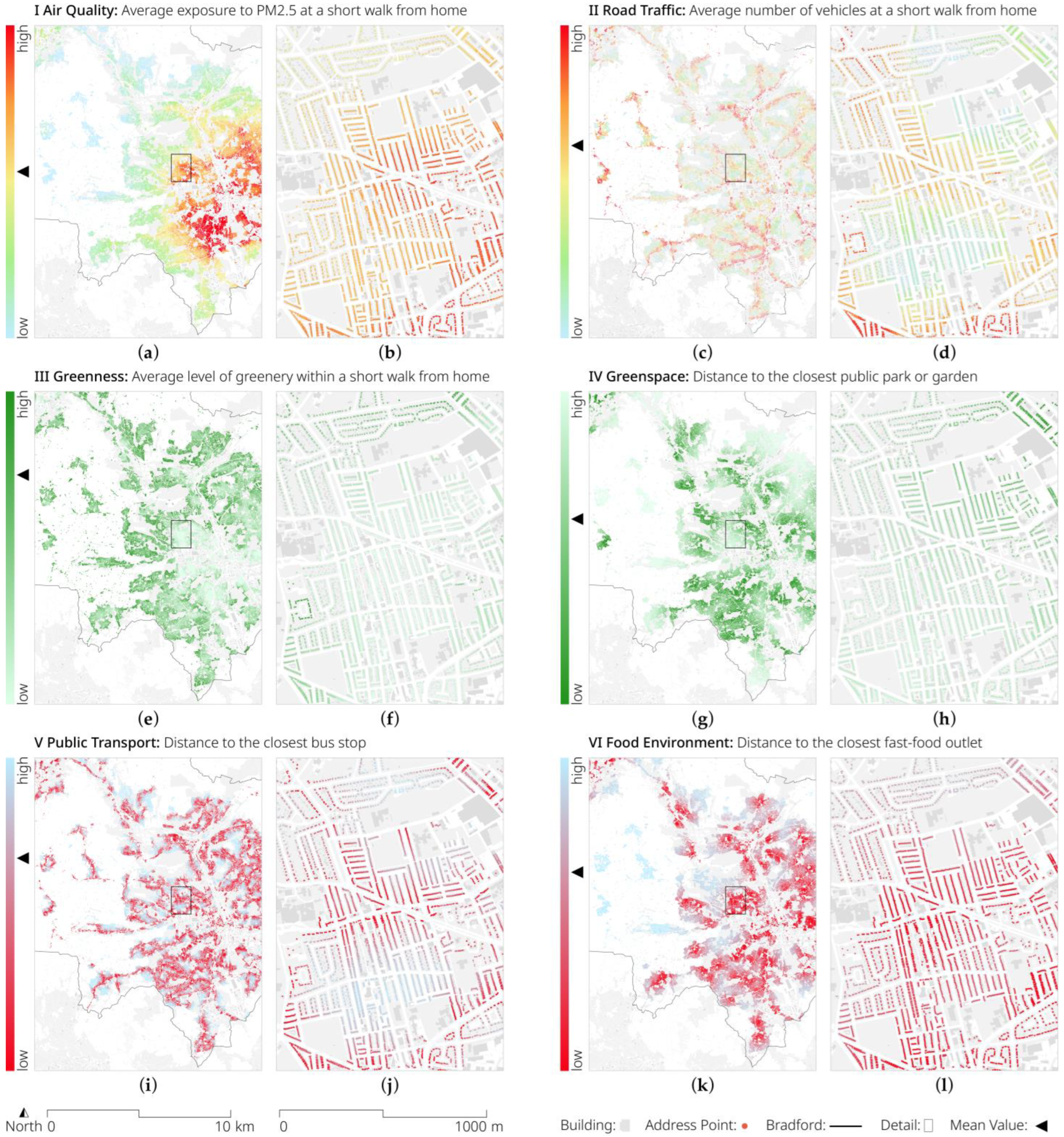
| I | Avg. exposure to PM 2.5 at a short walk from home (μg/m3) | 8.92 | 0.98 | 6.40 | 11.48 | 9.01 | 10.31 |
| II | Avg. number of vehicles at a short walk from home (AM) | 188.72 | 182.93 | 0.00 | 2268.00 | 141.00 | 0.00 |
| III | Avg. level of greenery within a short walk from home | 0.22 | 0.06 | 0.08 | 0.44 | 0.22 | 0.12 |
| IV | Distance to the closest public park or garden (m) | 1044.94 | 708.12 | 10.54 | 5715.32 | 889.26 | 1105.96 |
| V | Distance to the closest bus stop (m) | 216.52 | 155.05 | 10.05 | 4338.08 | 182.99 | 268.05 |
| VI | Distance to the closest fast-food outlet (m) | 763.99 | 739.79 | 10.32 | 5869.15 | 561.89 | 298.47 |
| VII | Diversity of shops within a short walk from home | 0.08 | 0.07 | 0.01 | 0.51 | 0.06 | 0.33 |
| VIII | Avg. level of walkability within a short walk from home | 0.86 | 0.37 | 0.05 | 2.51 | 0.84 | 2.03 |
| IX | Closeness to other things in the city within 1 km | 1578.83 | 931.49 | 0.36 | 5986.89 | 1419.43 | 4157.30 |
| X | Height of the home building (m) | 6.55 | 3.88 | 0.10 | 39.60 | 5.70 | 5.40 |
| XI | Size of the home (sqm) | 88.87 | 49.56 | 0.00 | 3384.00 | 78.00 | 70.00 |
| Dataset | 2013 | 2014 | 2015 | 2016 | 2017 | 2018 | 2019 | 2020 | 2021 | 2022 |
|---|---|---|---|---|---|---|---|---|---|---|
| OS MasterMap |  | | | | | | | | | |
| OS Highways (OS ITN) | () | () | () | | | | | | | |
| OS Urban Paths |  | | | | | | | | | |
| OS AddressBase Prem. | | | | | | | | | | |
| OS POI | | | | | | | | | | |
| OS Open Greenspace | | | | | | | | | | |
| USGS Landsat 8 | | | | | | | | | | |
| EPC | | | | | | | | | | |
| DEFRA (LA modelling) | | | | | | () | () | () | () | () |
| Trafficmaster | | | | | | | | | | |
| NaPTAN | | | | | | | | | | |
’: dataset is available, ‘()’: only dataset in brackets available, and ‘’: dataset is not available.| Dataset | 2013 | 2014 | 2015 | 2016 | 2017 | 2018 | 2019 | 2020 | 2021 | 2022 |
|---|---|---|---|---|---|---|---|---|---|---|
| NCDS | | | | | | | | | | |
| BCS70 | | | | | | | | | | |
| UKHLS | | | | | | | | | | |
| BHPS | | | | | | | | | | |
| MCS | | | | | | | | | | |
| Next Steps (LSYPE) | | | | | | | | | | |
’: dataset is available, and ‘’: dataset is not available.Disclaimer/Publisher’s Note: The statements, opinions and data contained in all publications are solely those of the individual author(s) and contributor(s) and not of MDPI and/or the editor(s). MDPI and/or the editor(s) disclaim responsibility for any injury to people or property resulting from any ideas, methods, instructions or products referred to in the content. |
© 2023 by the authors. Licensee MDPI, Basel, Switzerland. This article is an open access article distributed under the terms and conditions of the Creative Commons Attribution (CC BY) license (https://creativecommons.org/licenses/by/4.0/).
Share and Cite
Krenz, K.; Dhanani, A.; McEachan, R.R.C.; Sohal, K.; Wright, J.; Vaughan, L. Linking the Urban Environment and Health: An Innovative Methodology for Measuring Individual-Level Environmental Exposures. Int. J. Environ. Res. Public Health 2023, 20, 1953. https://doi.org/10.3390/ijerph20031953
Krenz K, Dhanani A, McEachan RRC, Sohal K, Wright J, Vaughan L. Linking the Urban Environment and Health: An Innovative Methodology for Measuring Individual-Level Environmental Exposures. International Journal of Environmental Research and Public Health. 2023; 20(3):1953. https://doi.org/10.3390/ijerph20031953
Chicago/Turabian StyleKrenz, Kimon, Ashley Dhanani, Rosemary R. C. McEachan, Kuldeep Sohal, John Wright, and Laura Vaughan. 2023. "Linking the Urban Environment and Health: An Innovative Methodology for Measuring Individual-Level Environmental Exposures" International Journal of Environmental Research and Public Health 20, no. 3: 1953. https://doi.org/10.3390/ijerph20031953
APA StyleKrenz, K., Dhanani, A., McEachan, R. R. C., Sohal, K., Wright, J., & Vaughan, L. (2023). Linking the Urban Environment and Health: An Innovative Methodology for Measuring Individual-Level Environmental Exposures. International Journal of Environmental Research and Public Health, 20(3), 1953. https://doi.org/10.3390/ijerph20031953