Article

Temporal Characteristics of Ozone (O3) in the Representative City of the Yangtze River Delta: Explanatory Factors and Sensitivity Analysis

1
College of Environment, Zhejiang University of Technology, Hangzhou 310023, China
2
National Institute of Metrology, Beijing 102200, China
3
Shaoxing Ecological and Environmental Monitoring Center of Zhejiang Province, Shaoxing 312000, China
4
Hangzhou Xufu Detection Technology Co., Ltd., Hangzhou 310023, China
*
Authors to whom correspondence should be addressed.
Int. J. Environ. Res. Public Health 2023, 20(1), 168; https://doi.org/10.3390/ijerph20010168
Submission received: 15 November 2022 / Revised: 7 December 2022 / Accepted: 19 December 2022 / Published: 22 December 2022
(This article belongs to the Special Issue Risk Characterization of Environmental/Human Health)

Abstract

:
Ozone (O3) has attracted considerable attention due to its harmful effects on the ecosystem and human health. The Yangtze River Delta (YRD), China in particular has experienced severe O3 pollution in recent years. Here, we conducted a long-term observation of O3 in YRD to reveal its characteristics. The O3 concentration in autumn was the highest at 72.76 ppb due to photochemical contribution and local convection patterns, with its lowest value of 2.40 ppb in winter. O3 exhibited strong diurnal variations, showing the highest values in the early afternoon (15:00–16:00) and the minimum in 07:00–08:00, specifically, peroxyacetyl nitrate (PAN) showed similar variations to O3 but PAN peak usually occurred 1 h earlier than that of O3 due to PAN photolysis. A generalized additive model indicated that the key factors to O3 formation were NO2, PAN, and temperature. It was found that a certain temperature rise promoted O3 formation, whereas temperatures above 27 °C inhibited O3 formation. An observation-based model showed O3 formation was VOCs-limited in spring and winter, was NOx-limited in summer, and even controlled by both VOCs and NOx in autumn. Thus, prevention and control strategies for O3 in the YRD are strongly recommended to be variable for each season based on various formation mechanisms.

1. Introduction

O3 is a typical secondary pollutant with a complex formation mechanism involving a series of chemical reactions among volatile organic compounds (VOCs), oxides of nitrogen (NOx, NO + NO2) and carbon monoxide (CO) [1]. O3, as an important indicator of photochemical pollution, plays a central role in the oxidation of chemical and climate-relevant trace gases in the troposphere [2]. O3 pollution has become a serious air quality problem affecting human health, vegetation, biodiversity, and climate worldwide as O3 concentrations have increased significantly since the second half of the 20th century [3,4]. According to a government report in China in 2020, O3 is the only air pollutant that maintained a rising trend during the last 5 years and O3 pollution is another urgent environmental problem in China, except for haze [5].
It has been noted that O3 levels increased by 30% to 70% in the temperate and polar regions of the Northern Hemisphere from 1896–1975 [3]. Despite policies to reduce precursor emissions, O3 concentrations have remained high; therefore, in-depth studies of the factors influencing O3 formation are critical to controlling ozone pollution. In addition to precursor substances, meteorological factors also have an influential effect on ambient O3 concentration [6,7]. Peroxyacetyl nitrate (CH3C(O)O2NO2, PAN) in the atmosphere serves also as a reliable and scientific indicator of photochemical pollution [8]. PAN acts as a temporary reservoir for NOx and radicals, which can be transported to distant areas to redistribute NOx as well as influence O3 production on a regional or even global scale [9]. Recently, some related studies focused on severe photochemical smog events in China with a relatively short period of measurement [10,11], but most of them focused on the events occurring in Beijing and the Pearl River Delta (PRD), China [10,12,13].
The Yangtze River Delta (YRD) is the region with the highest degree of urbanization and industrialization in China, and the coal-based energy system not only supports urbanization and industrialization but also contributes to serious regional air pollution problems [14]. Since 2017, O3 has become the most significant air pollutant in the YRD [5]. As the integrated development of the YRD has become a national strategy [15], the new situation of air pollution prevention and control makes it necessary to conduct an in-depth study on the O3 characteristics in the YRD to promote the sustainable development of the YRD.
So far, researchers have studied the spatial and temporal variations of O3, the mechanism of its formation, and the influencing factors [16,17,18]. Previous research has shown that O3 in the upper troposphere has increased annually across Europe from 1995 to 2013 [19]. In the troposphere with little UV radiation, it has been widely established that NO2 photolysis at wavelengths ≤424 nm becomes the main source of atomic oxygen and contributes to O3 formation. The main feature of O3 formation is the nonlinear dependence of O3 production on its precursors, i.e., NOx and VOCs [2]. Several studies have proven that there is a complex photochemical interaction between O3 and PM 2.5 and that PAN photochemistry has both negative and positive effects on O3 production [2,9]. In addition, some studies have found that the correlation between O3 and meteorological factors varies by season and region [16].
Generally, the available literature provides an essential foundation for ozone research. However, many studies focused on a single air pollutant, and few considered the synergistic and coordinated effects of multiple pollutants in a comprehensive manner [15]. Thus, in this study, we performed a one-year continuous observation of O3, PAN, other pollutants, and meteorological parameters to provide further insights into the formation mechanism of ambient O3 in the YRD, China in 2021 in a typical city located in the YRD, China, Shaoxing city, which is the core city of the Great Hangzhou Bay Area, near Shanghai and Hangzhou [20]. Here, a generalized additive model (GAM) was used to synthetically quantify the complex nonlinear relationships between O3 and multiple parameters, specifically including PAN for the first time. Compared with machine learning techniques, the GAM can uniquely quantify trends in O3 concentrations, which is better for understanding and controlling pollution [16]. Additionally, an observation-based model (OBM) was used to investigate the sensitivity of O3 production in different seasons, evaluating the effects of precursor reduction on O3 production. Therefore, this study can provide a comprehensive understanding of O3 formation and scientific evidence for the prevention and control of O3 pollution in the YRD, China.

2. Materials and Methods

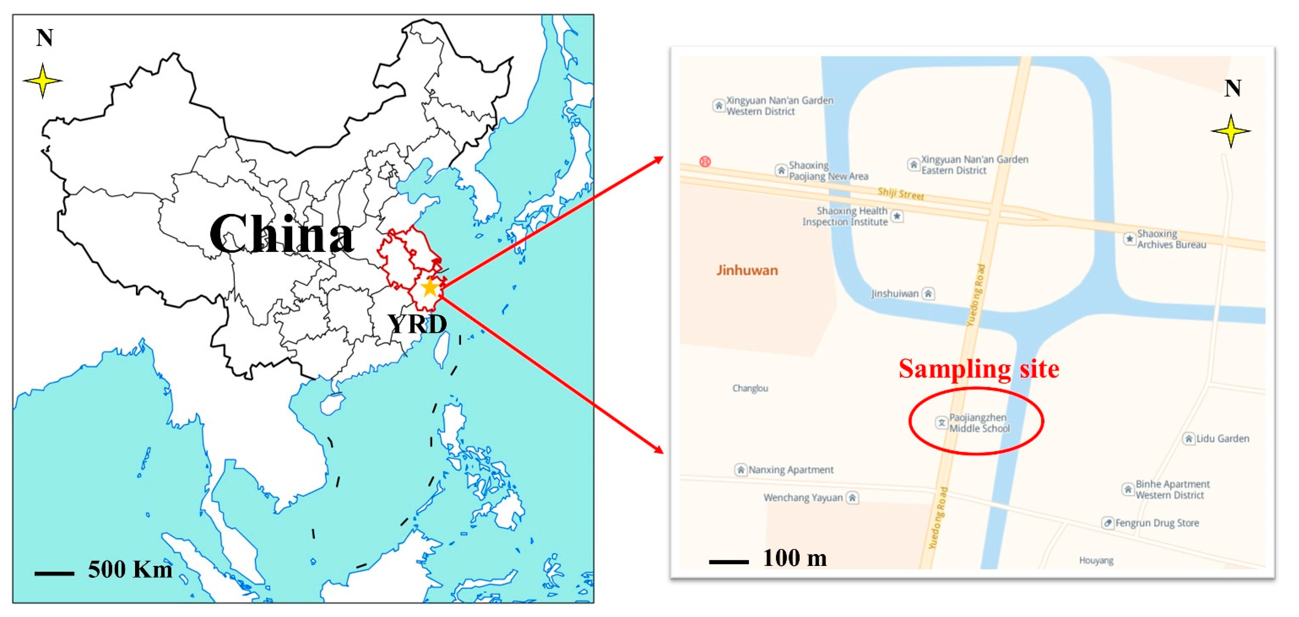
2.1. Observation Site

A field observing campaign was continuously conducted from January–December 2021 at an Atmospheric Observation Supersite (120.62° E, 30.08° N) in Shaoxing shown in Figure 1, located on the rooftop of an approximately 15 m-high building. The observation site is surrounded by residential areas and administrative offices, with well-developed traffic and no obvious industrial pollution sources, which can be considered as a typical urban site in the YRD, China. March, April, and May are considered as spring season, June, July, and August as summer, September, October, and November as autumn, and December, January, and February as winter in this paper according to the climate in YRD, China.

2.2. Measurement Apparatus and Methods

Concentrations of atmospheric O3, NOx, SO2, and CO were measured by instruments (USA i-series 49i, 42i, 43i, and 48i, Thermo Fisher Scientific, Waltham, MA, USA), while PM2.5 is sampled on a tapered element oscillating microbalance (TEOM1405, Thermo Fisher Scientific, Waltham, MA, USA). We calibrated each of these instruments periodically on a monthly basis. Meteorological data (temperature (T) and relative humidity (RH)) were obtained from an on-site meteorological station.
PAN concentration was determined through a PAN analyzer (PAN, Met Con Inc., SN, German) containing gas chromatography with an electron capture detector (GC-ECD), a sampling and calibration unit, and a computer control unit. It is the reaction of NO and acetone under UV light to produce PAN standard gas. During the observation period, calibration was performed once a week. The PAN was detected every 5 min with a detection limit of 50 ppt. The overall uncertainty of the measurement was estimated to be ± 3%.
Ambient VOCs were measured online by a cryogen-free automated gas chromatography (GC) system equipped with a flame ionization detector (FID) and mass spectrometer detector (MSD) with a temporal resolution of 1 h (Lu et al., 2022). A total of 94 VOC components were identified and measured during the course of this study. Detailed descriptions of the principles, performance, quality assurance, and quality control (QA/QC) processes of the online GC-MS/FID system are available in a previously published paper [20].

2.3. Generalized Additive Model

GAM, an extension of the additive model, is a flexible and free regression model that can make more reasonable nonlinear fittings than traditional statistical models [21]. It is widely used to reveal the complex nonlinear relationships between air pollutants and contributing factors in some air pollution studies [22,23]. In this study, GAM was applied to analyze the relationship between O3 and some factors including PAN, VOCs, PM2.5, NO, NO2, CO, T, and RH, respectively. Its basic form is as follows [24]:
g μ = α + f 1 x 1 + f 2 x 2 + f n x n + β
where μ is the response variable; g μ is the “link” function; α is the intercept; x 1 , x 2 , and x n are the impact factors; f 1 x 1 , f 1 x 1 , and f n x n are the smooth functions of the impact factors; and β is the residual.

2.4. Observation-Based Model

An observation-based model (OBM) was used to simulate the net O3 production rate and the sensitivity mechanism of O3 production in this study [25]. The model is informed by observations of 94 VOCs, trace gases (O3, NOx, and CO), and the meteorological parameter as boundary conditions for simulating atmospheric photochemical processes. The relative incremental response (RIR) was calculated using Equation (2) to evaluate the relative contribution of the precursors to O3 formation [18]:
R I R X = P O 3 X P O 3 X Δ X P O 3 X Δ S X S X
where, X represents a specific precursor of O3, including VOCs, NOx, and CO, respectively. P O 3 is the O3 formation potential from 07:00 a.m. to 19:00 p.m., which is the net amount of O3 production rate during the evaluation period and can be obtained from the OBM; Δ X represents the change in X concentration; S X means the observed concentrations of species X , which represents the combined impacts of regional traffic and on-site emissions; Δ S X S X means the relative change of S X [26].

3. Results and Discussion

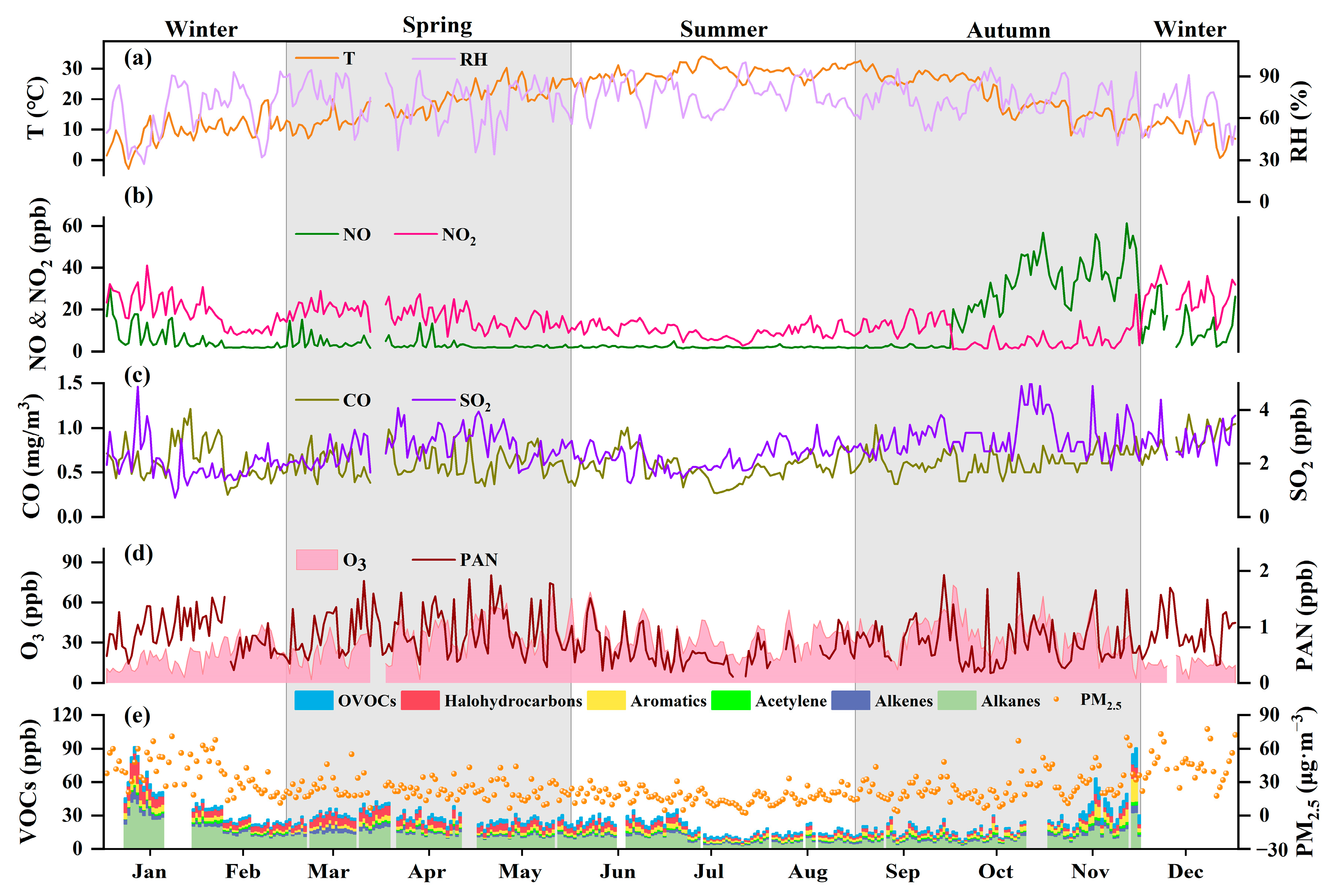
3.1. Temporal Variations of Ambient O3 and Related Parameters

3.1.1. Seasonal Variation

The temporal variations and statistical description of each observed element during the observation period are displayed in Figure 2 and Table 1, respectively. The measured daily mean concentrations of O3 ranged from 2.40 to 72.76 ppb, with an annual average of 30.27 ppb, which was higher than those reported in other cities such as Xiamen (28.11 ppb) [27], Shenzhen (27.3 ppb) [28], and Melbourne (20 ppb) [29]. The annual levels of PAN, VOCs, NO, NO2, and SO2 were 0.81 ppb, 26.18 ppb, 9.18 ppb, 13.82 ppb, and 2.55 ppb, respectively. The levels of PM2.5 and CO were 26.66 μg·m−3 and 0.62 mg·m−3, respectively.
The mean concentration of O3 in autumn (36.16 ppb) was significantly higher than in all other seasons, with the maximum daily concentration also occurring in autumn (72.76 ppb), unlike in Chengdu and Beijing, but the same as the previous result from Shanghai in the YRD [17,27,30]. It reflects the local synoptic flow pattern, which is the product of the interaction of the East Asian monsoon, tropical cyclones, and the land–sea breezes over the YRD [31]. The average O3 concentration was the lowest in winter, which was due to weaker photochemical reactions at low ultraviolet radiation. Figure 2 shows there is a significant correlation between O3 and PAN (p < 0.05), but the lowest mean PAN concentration occurred in summer (0.59 ppb). It was explained by the location of the observatory in the YRD, which was influenced by the East Asian summer monsoon that brought clean, humid air masses and diluted PAN, none of which were conducive to photochemical production (Li and Fan, 2022). It is noteworthy that the PAN had the highest average level in the spring (0.94 ppb), which was inconsistent with some previous reports [32,33]. We attribute this to low photodegradation efficiency and accumulation of long-term non-methane volatile organic compounds (NMVOCs) in the free troposphere during winter [34,35]. Photochemistry became active in early spring and accumulated NMVOCs promoted PAN accumulation, resulting in the highest PAN levels in spring, matching the mean level of VOCs in this study, which was highest in winter (39.03 ppb).
The averaged values for PM2.5, NO2, and CO were significantly higher in winter than in other seasons, at 40.87 ppb, 21.46 ppb, and 0.71 ppb, respectively. It could be caused by weak convection in the winter, leading to higher concentrations of accumulated pollutants [36]. NO and SO2 were concordant with O3, with average concentrations highest in the autumn. Meanwhile, the ratio value of NO/NO2 was greater than 1.0 (3.05), indicating that less O3 consumption occurred in the NO2 photolysis cycle in autumn [37].

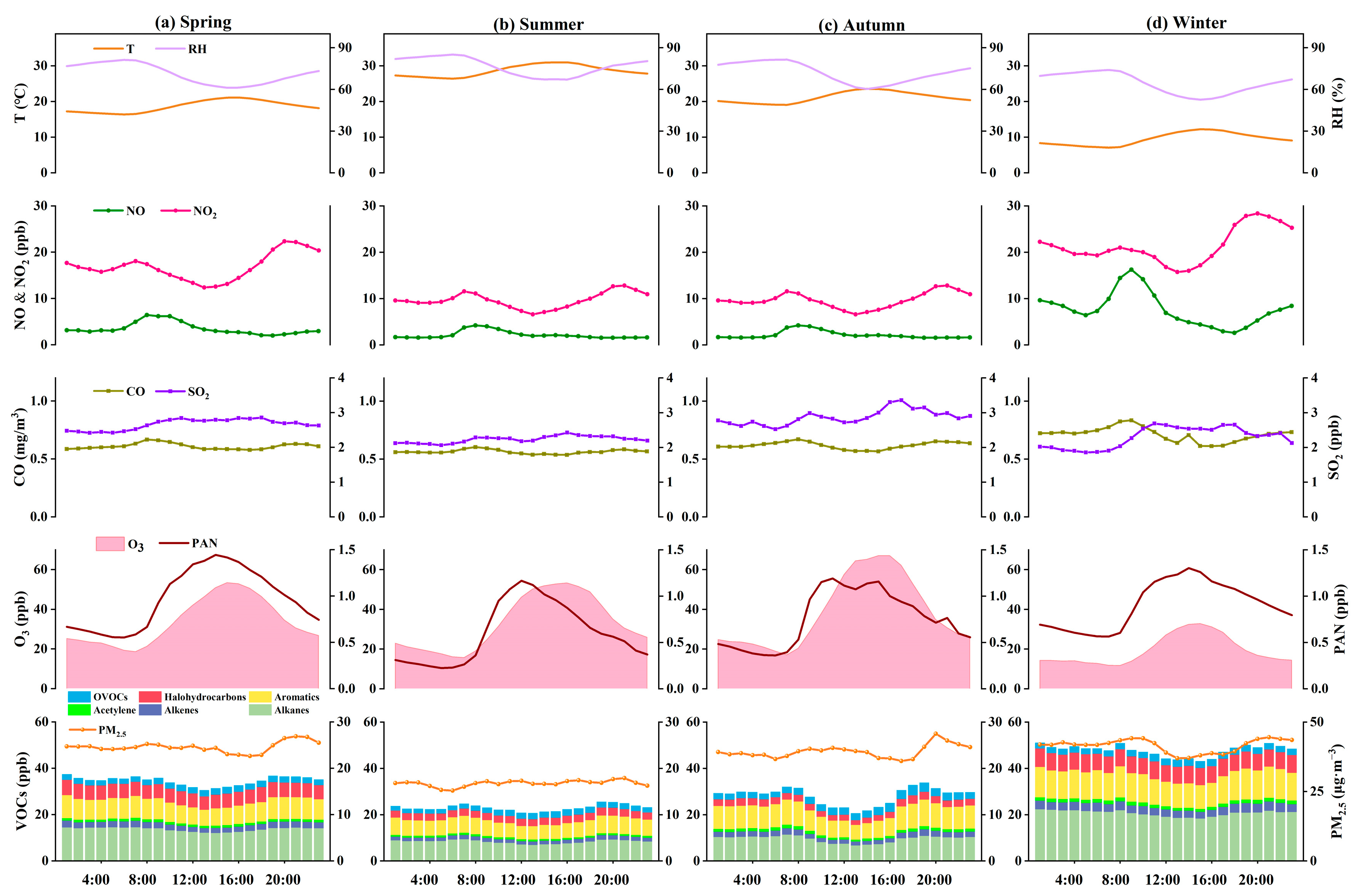
3.1.2. Diurnal Variation

The average diurnal variation patterns for O3, PAN, and some other pollutants as well as meteorological parameters during the 4 seasons of 2021 are shown in Figure 3. O3 as a secondary pollutant showed the highest value during the early afternoon (15:00–16:00) and the lowest value at 07:00–08:00. Temporal variations in solar radiation and temperature were considered major drivers of such diurnal variations in O3 levels [2]. PAN has a similar diurnal pattern to O3, reaching a maximum between 11:00 and 14:00 in all seasons, then decreasing during low solar radiation, and a minimum in the early morning (06:00–08:00, indicating the dominance of local photochemistry during the observation period [11]. Specifically, the PAN peak usually occurred 1 h earlier than that of O3, presumably resulting from the increasing decomposition rate of PAN with increasing temperature [27]. The variation between maximum and minimum values of PAN in summer was the highest (0.94 ppb) while was the smallest difference in winter (0.70 ppb), which was a net growth pattern that also indicates that the lifetime of PAN increases with decreasing temperature.
Contrastingly, NOx, CO, and VOCs levels showed a diurnal pattern opposite to O3 (Figure 3). The diurnal variation of NO2 exhibited a bimodal distribution, with a peak in the morning, followed by a decrease in NO2 concentration due to photolysis, and subsequent accumulation of NO2 at night due to primary emissions. The peak NOx and CO levels in the morning were strongly related to vehicle emissions during the morning rush hour. The trend of VOCs concentration was the same as the daily variation of NO2, with a higher concentration in the morning, followed by a gradual decrease, but then a higher concentration at night, which was associated with the lower photochemical losses at night and the accumulation of primary emissions of pollutants. Anyway, a close correlation between precursor emissions and human activities (e.g., transportation) can be seen in the observed areas.

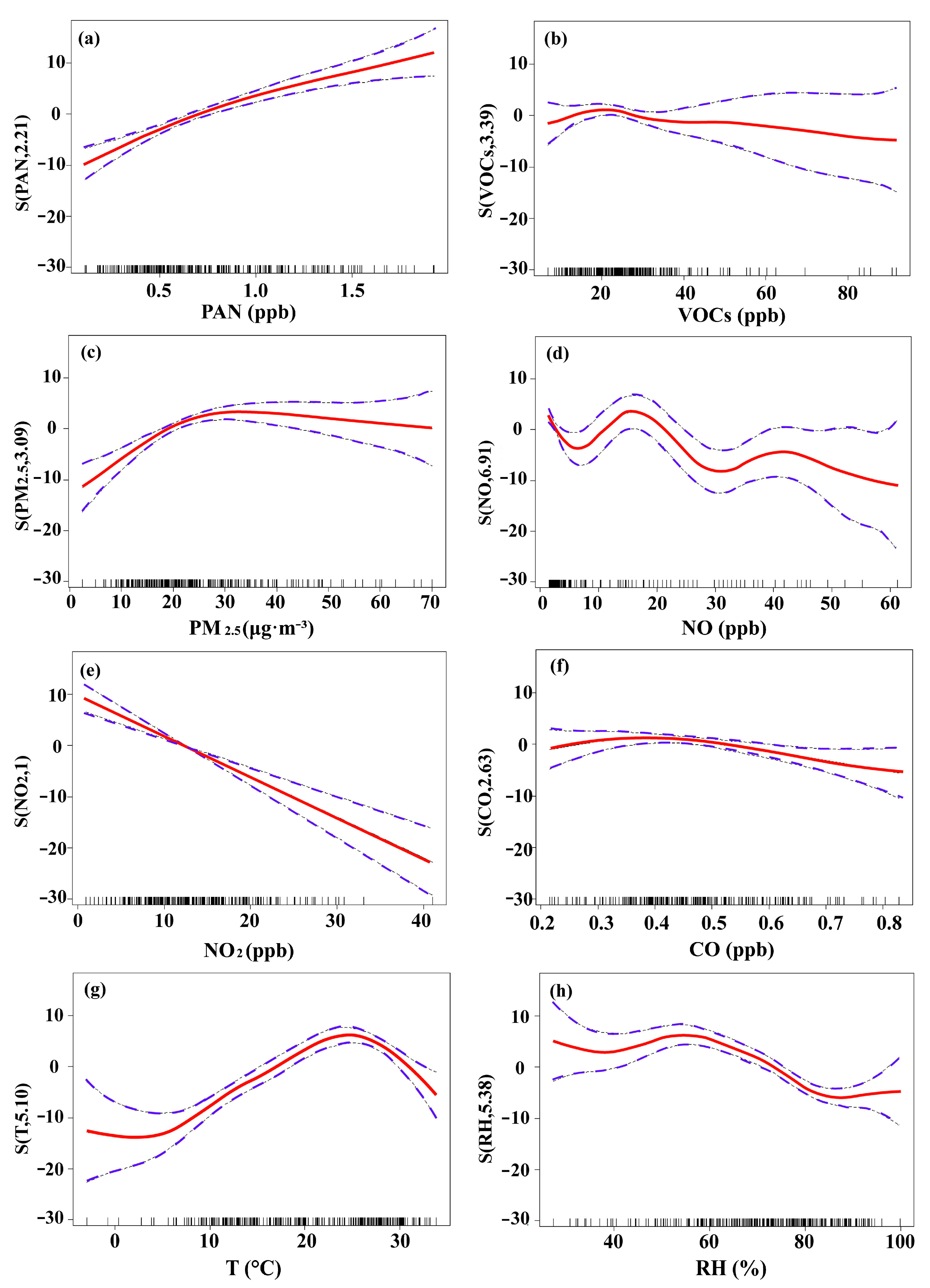
3.2. The Influencing Factors of O3 Using the GAM

Eight parameters were selected as explanatory variables (PAN, VOCs, PM2.5, NO, NO2, CO, T, RH) and O3 concentration as the response variable. The multi-factorial correlation analysis was performed using the GAM and the results are shown in Figure 4 and Table 2. g O 3 = 32.56 + f 1 N O 2 + f 2 P A N + f 3 T + f 4 R H + f 5 P M 2.5 + f 6 N O + f 7 C O + f 8 V O C s + 0.35 is the parameterized formula.
In accordance with the F values, explanatory variables over the monitoring period were in the order of NO2 (47.88) > PAN (24.22) > T (22.34) > RH (13.22) > PM2.5 (9.12) > NO (4.85) > CO (3.25) > VOCs (1.05). Notably, there was a significant negative correlation between NO2 and O3 (Figure 4e), which was consistent with previous results from Beijing [16], but the degree of freedom (df) of NO2 in this study was 1, indicating that a large proportion of O3 was directly produced by NO2 photolysis [38]. The effect of PAN on O3 was also not negligible, showing a nonlinear positive correlation between the two with a narrow confidence interval (CI) (Figure 4a). In general, PAN inhibits O3 formation by competing with O3 precursors and terminating free radical chain reactions [11]. However, the positive correlation results implied that PAN may also promote O3 production by providing more RO2 radicals and increasing the oxidation capacity of the atmosphere in the presence of sufficient NOx [33]. Therefore, controlling vehicle emissions can reduce NOx levels and effectively mitigate the O3-promoting effect of PAN.
The Edf of T and RH were both greater than 1 (Figure 4g,h), demonstrating a non-linear relationship with the response variable. When T < 27 °C, the O3 markedly increased with rising T, implying that a certain range of heating can promote the photochemical reaction of O3. In contrast to the direct linear relationship of many studies [16,39], the increase in temperature above 27 °C inhibited O3 formation. This inhibition of O3 formation at high temperatures was not a coincidence, as a similar situation was observed by the University of California [40]. This phenomenon was driven by atmospheric chemistry and ecosystem-climate interactions due to the strong function of an e-folding decrease of PAN at high temperatures, as well as in areas with strong sources of isoprene and NOx, where chemistry is more VOCs-limited could experience a decrease in O3 at high levels of temperature [40,41]. In addition, high temperatures may enhance surface heat flux and convective mixing, thereby increasing the atmospheric boundary layer height and diluting the O3 concentration [42]. When RH < 55%, the effect of RH on O3 concentrations did not change significantly, and when RH > 55%, O3 levels decreased remarkably with the increase of RH due to the interception effect of RH on precursors and the fact that O3 was dissolved in atmospheric water droplets and self-degraded at high relative humidity [43].
As levels of VOCs, PM2.5, and CO increased, O3 concentrations initially increased and then gradually decreased (Figure 4b,c,f). Higher PM2.5 levels contributed to increased O3 levels through the scattering effect of PM2.5 in a certain range, but excessively high PM2.5 levels reduced terrestrial ultraviolet, leading to the inhibition of photochemical reactions and hence lower O3 levels [21,44]. CO and VOCs had little effect on O3 and it seems reasonable to assume free radical reactions with NOx dominated in the region. NO displayed a complex relationship with O3, but was generally negatively correlated due to their susceptibility to reaction [2]. HO2 in a high-NO atmosphere promotes the oxidation of NO to NO2, and NO consumes peroxyacetyl radicals to generate NO2, promoting O3 formation [9,39]. In summary, the multifactorial GAM is more interpretable and simulates more realistic O3 trends in the atmosphere. It demonstrates that in the YRD NO2 and PAN have the greatest influence on O3 levels, followed by T and RH.

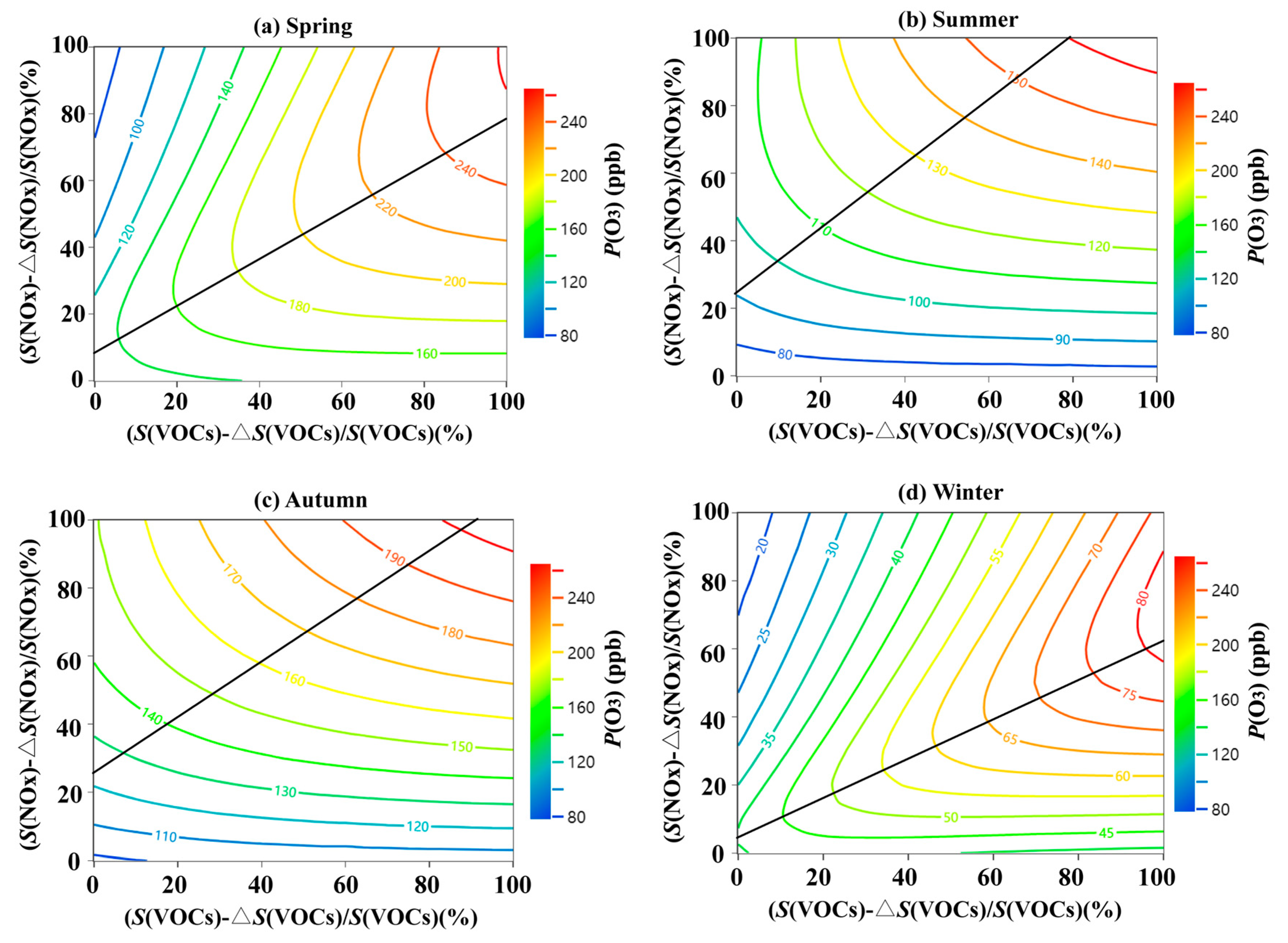
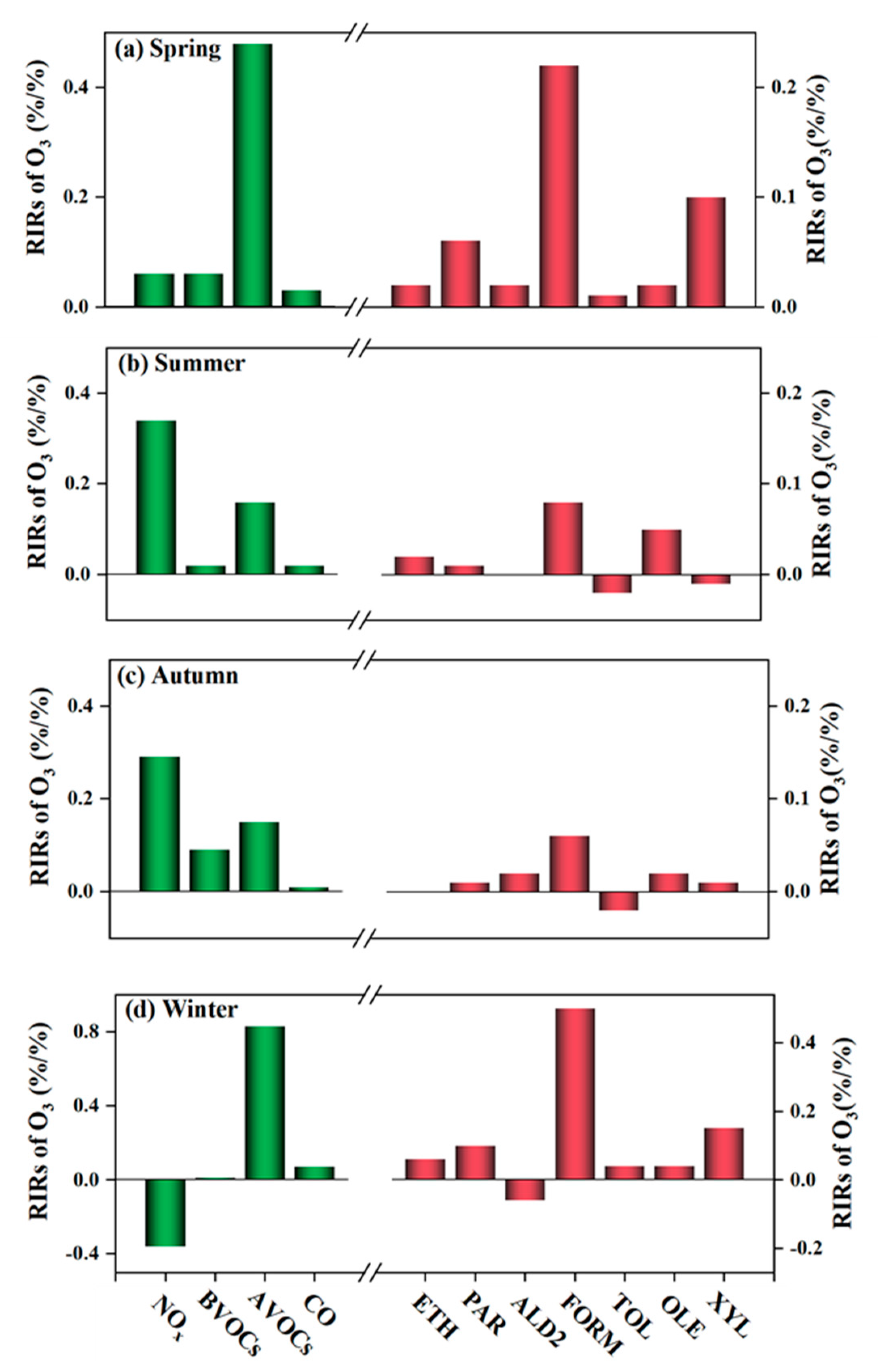
3.3. Sensitivity of O3 Formation

In this study, the RIR values calculated by OBM for the precursors in all seasons are shown in Figure 5. The RIR values for VOCs were significantly higher than those for NOx in spring and winter (Figure 5a,d), with a negative RIR value for NOx in the winter (−0.36), indicating O3 production in the observing area was mainly controlled by VOCs. Notably, the RIR of BVOC (isoprene) in winter was only 0.01, which can be attributed to the fact that plant branches became bare in winter and BVOC emissions were greatly reduced, which, together with low temperatures and weak radiation in winter, caused the effect of isoprene on O3 formation to be lower [45]. Moreover, formaldehyde (FORM) and xylene (XYL) showed the top two RIRs for O3 in spring and winter, revealing their dominance in the O3 generation. Therefore, reducing VOCs in these two seasons is more effective for controlling O3 pollution. Additionally, previous studies have concluded that anthropogenic primary sources (e.g., vehicle emissions and industrial activities) contributed most to FORM in the spring and winter, that biological sources contributed more in the summer and autumn, and that the major sources of XYL were traffic and industry [46,47]. O3 production in summer was more sensitive to NOx, with a RIR of 0.34. Toluene (TOL) and XYL of AVOCs appeared to have negative values and decreases in their concentrations will instead lead to an increase in O3 concentrations. In autumn, O3 formation displayed a high sensitivity to simultaneously VOCs and NOx (RIR(VOCs): 0.24, RIR(NOx): 0.29), while the effect of CO on O3 formation was negligible (RIR(CO): 0.01). Further analysis showed reducing TOL has an adverse impact on O3 formation and FORM needs to be prevented and controlled. In a nutshell, O3 formation was in the VOCs-limited in spring and winter, controlled by NOx in summer, and even controlled by both VOCs and NOx in autumn, and FORM emissions have to be emphasized throughout the year.
Empirical Kinetics Modeling Approach curves were simulated and plotted to investigate the impacts of precursors reduction on O3 formation (Figure 6). In other words, the relationship of P(O3) with relative changes of S(VOCs) and S(NOx) can be expressed by isopleth diagrams for P(O3). The mean P(O3) levels varied considerably over the four seasons, with estimates of 262 ppb, 165 ppb, 205 ppb, and 77 ppb, respectively. In spring, a 10% reduction in S(VOCs) resulted in a decrease of 13 ppb in P(O3), and a 10% reduction in NOx only resulted in a reduction of 2 (Figure 6a). In winter, O3 levels gradually decreased with an increasing reduction ratio when only VOCs was reduced; however, O3 levels progressively increased when only NOx was reduced, especially when the reduction ratio reached to 40% (Figure 6d). It indicated that the regime was in the VOCs-limited in spring and winter as the results of the RIRs. During summer, O3 formation was more sensitive to NOx, with an increase in the percentage of NOx reduction leading to a notable reduction in O3 levels, while VOCs reduction required a large percentage of reduction. For autumn, the S(VOCs) and S(NOx) data point was close to the ridge line, indicating the point was in a transition regime where significant NOx reductions can be achieved in the short term but easily transition to the NOx-limited regime. Thus, stringent control of VOCs pollution ought to be implemented in parallel with collaborative regional prevention and control of NOx to facilitate long-term control of O3. However, many studies have not studied the seasonal sensitivity differences in depth and finally only obtained that the study area was in the VOCs-limited control or NOx-limited [48,49]. Based on the above conclusions, it is necessary for YRD to dynamically adjust its prevention and control strategy in accordance with the characteristics of the O3 formation mechanism.

4. Conclusions

Long-term O3 observations in the YRD in 2021 displayed strong seasonal variations with a maximum in autumn (72.76 ppb) due to the metrological interaction and the lowest O3 level in the low-radiation winter (19.03 ppb). O3 levels displayed an obvious cyclic pattern of diurnal variation, with O3 showing the highest values in the early afternoon (15:00–16:00) due to vivid photochemical reactions and the lowest values in the 07:00–08:00. PAN presented a similar diurnal pattern to O3; however, the rate of decomposition of PAN increased with increasing temperature, resulting in the peak of PAN usually occurring 1 h earlier than the peak of O3 precursors (NOx, CO, and VOCs), which, in contrast to O3, showed a diurnal pattern, with the lowest levels in the afternoon and the maximum in the night or the morning peak.
Furthermore, GAM revealed key factors affecting O3 levels were NO2, PAN, and T. A large fraction of O3 was produced directly by NO2 photolysis, and PAN contributes to O3 production by providing more RO2 radicals and increasing the oxidation capacity of the atmosphere in the presence of sufficient NOx. Thus, reducing vehicle NOx emissions can effectively mitigate the O3-promoting effect of PAN. It was found a certain temperature rise promoted the photochemical reaction of O3, whereas rising temperatures above 27 °C inhibited O3 formation. It is strongly recommended to target control in different seasons according to various O3 formation mechanisms. Based on the RIRs, FORM needs to be emphasized all year round.
This study extends the understanding of O3 pollution in the YRD region, integrates the coordinated effects of multiple parameters on O3 production, and quantifies the contribution of PAN to O3 formation for the first time, and proposes seasonal control of various precursors which are significant guidelines for photochemical pollution control in the YRD region, China.

Author Contributions

Conceptualization, Y.L. and X.P.; data curation, Y.L.; formal analysis, Y.L. and Z.W.; funding acquisition, X.P., H.W. and J.C.; investigation, B.X., J.L. and Q.X.; project administration, H.W. and J.C.; software, Y.L.; resources, D.S.; supervision, X.P.; visualization, B.X., J.L. and Q.X.; writing—original draft, Y.L.; writing—review and editing, Y.L., Z.W., X.P. and D.S. All authors have read and agreed to the published version of the manuscript.

Funding

The APC was funded by the National Key Research and Development Program of China (2021YFF0600202 and 2022YFC3703500), the National Natural Science Foundation of China (41727805), the “Lead Goose” Research and Development Program of Zhejiang Province (2022C03073), the Key Research Program of Zhejiang Province (2021C03165), the Natural Sciences Foundation of Zhejiang Province (LZ20D050002), the Science and Technology Plan Special Program of Shaoxing City (2022B41006).

Data Availability Statement

The data presented in this study are available on request from the corresponding author. The data are not publicly available due to privacy.

Conflicts of Interest

Author Dongfeng Shi was employed by the company Hangzhou Xufu Detection Technology Co., Ltd. The remaining authors declare that the research was conducted in the absence of any commercial or financial relationships that could be construed as a potential conflict of interest.

References

  1. Xue, L.K.; Wang, T.; Gao, J.; Ding, A.J.; Zhou, X.H.; Blake, D.R.; Wang, X.F.; Saunders, S.M.; Fan, S.J.; Zuo, H.C.; et al. Ground-level ozone in four Chinese cities: Precursors, regional transport and heterogeneous processes. Atmos. Chem. Phys. 2014, 14, 13175–13188. [Google Scholar] [CrossRef] [Green Version]
  2. Wang, T.; Xue, L.; Brimblecombe, P.; Lam, Y.F.; Li, L.; Zhang, L. Ozone pollution in China: A review of concentrations, meteorological influences, chemical precursors, and effects. Sci. Total Environ. 2017, 575, 1582–1596. [Google Scholar] [CrossRef] [PubMed]
  3. Agathokleous, E.; Feng, Z.; Oksanen, E.; Sicard, P.; Wang, Q.; Saitanis, C.J.; Araminiene, V.; Blande, J.D.; Hayes, F.; Calatayud, V.; et al. Ozone affects plant, insect, and soil microbial communities: A threat to terrestrial ecosystems and biodiversity. Sci. Adv. 2020, 6, eabc1176. [Google Scholar] [CrossRef] [PubMed]
  4. Sicard, P. Ground-level ozone over time: An observation-based global overview. Curr. Opin. Environ. Sci. Health 2021, 19, 100226. [Google Scholar] [CrossRef]
  5. Wang, M.; Chen, W.; Zhang, L.; Qin, W.; Zhang, Y.; Zhang, X.; Xie, X. Ozone pollution characteristics and sensitivity analysis using an observation-based model in Nanjing, Yangtze River Delta Region of China. J. Environ. Sci. 2020, 93, 13–22. [Google Scholar] [CrossRef]
  6. Liu, H.; Liu, J.; Liu, Y.; Yi, K.; Yang, H.; Xiang, S.; Ma, J.; Tao, S. Spatiotemporal variability and driving factors of ground-level summertime ozone pollution over eastern China. Atmos. Environ. 2021, 265, 118686. [Google Scholar] [CrossRef]
  7. Coates, J.; Mar, K.A.; Ojha, N.; Butler, T.M. The influence of temperature on ozone production under varying NOx conditions – a modelling study. Atmos. Chem. Phys. 2016, 16, 11601–11615. [Google Scholar] [CrossRef] [Green Version]
  8. Han, J.; Lee, M.; Shang, X.; Lee, G.; Emmons, L.K. Decoupling peroxyacetyl nitrate from ozone in Chinese outflows observed at Gosan Climate Observatory. Atmos. Chem. Phys. 2017, 17, 10619–10631. [Google Scholar] [CrossRef] [Green Version]
  9. Liu, T.; Chen, G.; Chen, J.; Xu, L.; Li, M.; Hong, Y.; Chen, Y.; Ji, X.; Yang, C.; Chen, Y.; et al. Seasonal characteristics of atmospheric peroxyacetyl nitrate (PAN) in a coastal city of Southeast China: Explanatory factors and photochemical effects. Atmos. Chem. Phys. 2022, 22, 4339–4353. [Google Scholar] [CrossRef]
  10. Zhang, B.; Zhao, X.; Zhang, J. Characteristics of peroxyacetyl nitrate pollution during a 2015 winter haze episode in Beijing. Environ. Pollut. 2019, 244, 379–387. [Google Scholar] [CrossRef]
  11. Zeng, L.; Fan, G.-J.; Lyu, X.; Guo, H.; Wang, J.-L.; Yao, D. Atmospheric fate of peroxyacetyl nitrate in suburban Hong Kong and its impact on local ozone pollution. Environ. Pollut. 2019, 252, 1910–1919. [Google Scholar] [CrossRef] [PubMed]
  12. Xia, S.; Huang, X.; Han, H.; Li, X.; Yu, G. Influence of thermal decomposition and regional transport on atmospheric peroxyacetyl nitrate (PAN) observed in a megacity in southern China. Atmos. Res. 2022, 272, 106146. [Google Scholar] [CrossRef]
  13. Cui, M.; An, X.Q.; Sun, Z.B.; Wang, B.Z.; Wang, C.; Ren, W.J.; Li, Y.J. Characteristics and Meteorological Conditions of Ozone Pollution in Beijing. Ecol. Environ. Monit. Three Gorges 2022, 4, 25–35. [Google Scholar]
  14. Hong, Y.; Xu, X.; Liao, D.; Ji, X.; Hong, Z.; Chen, Y.; Xu, L.; Li, M.; Wang, H.; Zhang, H.; et al. Air pollution increases human health risks of PM2.5-bound PAHs and nitro-PAHs in the Yangtze River Delta, China. Sci. Total Environ. 2021, 770, 145402. [Google Scholar] [CrossRef] [PubMed]
  15. Lin, H.; Zhu, J.; Jiang, P.; Cai, Z.; Yang, X.; Yang, X.; Zhou, Z.; Wei, J. Assessing drivers of coordinated control of ozone and fine particulate pollution: Evidence from Yangtze River Delta in China. Environ. Impact Assess. Rev. 2022, 96, 106840. [Google Scholar] [CrossRef]
  16. Xu, T.; Zhang, C.; Liu, C.; Hu, Q. Variability of PM2.5 and O3 concentrations and their driving forces over Chinese megacities during 2018–2020. J. Environ. Sci. 2023, 124, 1–10. [Google Scholar] [CrossRef] [PubMed]
  17. Xiao, K.; Wang, Y.; Wu, G.; Fu, B.; Zhu, Y. Spatiotemporal Characteristics of Air Pollutants (PM10, PM2.5, SO2, NO2, O3, and CO) in the Inland Basin City of Chengdu, Southwest China. Atmosphere 2018, 9, 74. [Google Scholar] [CrossRef] [Green Version]
  18. Tan, Z.; Lu, K.; Jiang, M.; Su, R.; Dong, H.; Zeng, L.; Xie, S.; Tan, Q.; Zhang, Y. Exploring ozone pollution in Chengdu, southwestern China: A case study from radical chemistry to O3-VOC-NOx sensitivity. Sci. Total Environ. 2018, 636, 775–786. [Google Scholar] [CrossRef]
  19. Cohen, Y.; Petetin, H.; Thouret, V.; Marécal, V.; Josse, B.; Clark, H.; Sauvage, B.; Fontaine, A.; Athier, G.; Blot, R.; et al. Climatology and long-term evolution of ozone and carbon monoxide in the upper troposphere–lower stratosphere (UTLS) at northern midlatitudes, as seen by IAGOS from 1995 to 2013. Atmos. Chem. Phys. 2018, 18, 5415–5453. [Google Scholar] [CrossRef] [Green Version]
  20. Lu, Y.; Pang, X.; Lyu, Y.; Li, J.; Xing, B.; Chen, J.; Mao, Y.; Shang, Q.; Wu, H. Characteristics and sources analysis of ambient volatile organic compounds in a typical industrial park: Implications for ozone formation in 2022 Asian Games. Sci. Total Environ. 2022, 848, 157746. [Google Scholar] [CrossRef]
  21. Ma, Y.; Ma, B.; Jiao, H.; Zhang, Y.; Xin, J.; Yu, Z. An analysis of the effects of weather and air pollution on tropospheric ozone using a generalized additive model in western China: Lanzhou, Gansu. Atmos. Environ. 2020, 224, 117342. [Google Scholar] [CrossRef]
  22. Gujral, H.; Sinha, A. Association between exposure to airborne pollutants and COVID-19 in Los Angeles, United States with ensemble-based dynamic emission model. Environ. Res. 2021, 194, 110704. [Google Scholar] [CrossRef] [PubMed]
  23. Bi, Z.; Ye, Z.; He, C.; Li, Y. Analysis of the meteorological factors affecting the short-term increase in O3 concentrations in nine global cities during COVID-19. Atmos. Pollut. Res. 2022, 13, 101523. [Google Scholar] [CrossRef] [PubMed]
  24. Charles, J.S. Additive regression and other nonparametric models. Ann. Stat. 1985, 13, 689–705. [Google Scholar]
  25. Cardelino, C.A.; Chameides, W.L. An Observation-Based Model for Analyzing Ozone Precursor Relationships in the Urban Atmosphere. J. Air Waste Manage. Assoc. 1995, 45, 161–180. [Google Scholar] [CrossRef]
  26. Wang, J.; Zhang, Y.; Wu, Z.; Luo, S.; Song, W.; Wang, X. Ozone episodes during and after the 2018 Chinese National Day holidays in Guangzhou: Implications for the control of precursor VOCs. J. Environ. Sci. 2022, 114, 322–333. [Google Scholar] [CrossRef]
  27. Hu, B.; Liu, T.; Hong, Y.; Xu, L.; Li, M.; Wu, X.; Wang, H.; Chen, J.; Chen, J. Characteristics of peroxyacetyl nitrate (PAN) in a coastal city of southeastern China: Photochemical mechanism and pollution process. Sci. Total Environ. 2020, 719, 137493. [Google Scholar] [CrossRef]
  28. Yang, W.; Chen, H.; Wang, W.; Wu, J.; Li, J.; Wang, Z.; Zheng, J.; Chen, D. Modeling study of ozone source apportionment over the Pearl River Delta in 2015. Environ. Pollut. 2019, 253, 393–402. [Google Scholar] [CrossRef]
  29. Riley, M.L.; Watt, S.; Jiang, N. Tropospheric ozone measurements at a rural town in New South Wales, Australia. Atmos. Environ. 2022, 281, 119143. [Google Scholar] [CrossRef]
  30. Chen, Z.; Zhuang, Y.; Xie, X.; Chen, D.; Cheng, N.; Yang, L.; Li, R. Understanding long-term variations of meteorological influences on ground ozone concentrations in Beijing During 2006–2016. Environ. Pollut. 2019, 245, 29–37. [Google Scholar] [CrossRef]
  31. Cheng, L.; Wang, S.; Gong, Z.; Li, H.; Yang, Q.; Wang, Y. Regionalization based on spatial and seasonal variation in ground-level ozone concentrations across China. J. Environ. Sci. 2018, 67, 179–190. [Google Scholar] [CrossRef] [Green Version]
  32. Sun, M.; Zhou, Y.; Wang, Y.; Zheng, X.; Cui, J.; Zhang, D.; Zhang, J.; Zhang, R. Seasonal discrepancies in peroxyacetyl nitrate (PAN) and its correlation with ozone and PM2.5: Effects of regional transport from circumjacent industrial cities. Sci. Total Environ. 2021, 785, 147303. [Google Scholar] [CrossRef] [PubMed]
  33. Liu, Y.; Shen, H.; Mu, J.; Li, H.; Chen, T.; Yang, J.; Jiang, Y.; Zhu, Y.; Meng, H.; Dong, C.; et al. Formation of peroxyacetyl nitrate (PAN) and its impact on ozone production in the coastal atmosphere of Qingdao, North China. Sci. Total Environ. 2021, 778, 146265. [Google Scholar] [CrossRef]
  34. Zanis, P.; Ganser, A.; Zellweger, C.; Henne, S.; Steinbacher, M.; Staehelin, J. Seasonal variability of measured ozone production efficiencies in the lower free troposphere of Central Europe. Atmos. Chem. Phys. 2007, 7, 223–236. [Google Scholar] [CrossRef] [Green Version]
  35. Pandey Deolal, S.; Henne, S.; Ries, L.; Gilge, S.; Weers, U.; Steinbacher, M.; Staehelin, J.; Peter, T. Analysis of elevated springtime levels of Peroxyacetyl nitrate (PAN) at the high Alpine research sites Jungfraujoch and Zugspitze. Atmos. Chem. Phys. 2014, 14, 12553–12571. [Google Scholar] [CrossRef] [Green Version]
  36. Li, X.; Zhang, F.; Ren, J.; Han, W.; Zheng, B.; Liu, J.; Chen, L.; Jiang, S. Rapid narrowing of the urban–suburban gap in air pollutant concentrations in Beijing from 2014 to 2019. Environ. Pollut. 2022, 304, 119146. [Google Scholar] [CrossRef]
  37. Li, J.; Deng, S.; Tohti, A.; Li, G.; Yi, X.; Lu, Z.; Liu, J.; Zhang, S. Spatial characteristics of VOCs and their ozone and secondary organic aerosol formation potentials in autumn and winter in the Guanzhong Plain, China. Environ. Res. 2022, 211, 113036. [Google Scholar] [CrossRef]
  38. Clapp, L.J.; Jenkin, M.E. Analysis of the relationship between ambient levels of O3, NO2 and NO as a function of NOx in the UK. Atmos. Environ. 2001, 35, 6391–6405. [Google Scholar] [CrossRef]
  39. Diao, L.; Xiaohui, B.; Wenhui, Z.; Baoshuang, L.; Xuehan, W.; Linxuan, L.; Qili, D.; Yufen, Z.; Jianhui, W.; Yinchang, F. The characteristics of heavy ozone pollution episodes identification of the primary driving factors using a generalized additive model in an industrial megacity of northern, China. Atmosphere 2021, 12, 1517. [Google Scholar] [CrossRef]
  40. Steiner, A.L.; Davis, A.J.; Sillman, S.; Owen, R.C.; Michalak, A.M.; Fiore, A.M. Observed suppression of ozone formation at extremely high temperatures due to chemical and biophysical feedbacks. Proc. Natl. Acad. Sci. USA 2010, 107, 19685–19690. [Google Scholar] [CrossRef] [Green Version]
  41. Rasmussen, D.J.; Fiore, A.M.; Naik, V.; Horowitz, L.W.; Mcginnis, S.J.; Schultz, M.G. Surface ozone-temperature relationships in the eastern US: A monthly climatology for evaluating chemistry-climate models. Atmos. Environ. 2012, 47, 142–153. [Google Scholar] [CrossRef]
  42. Sudeepkumar, B.L.; Babu, C.A.; Varikoden, H. Atmospheric boundary layer height and surface parameters: Trends and relationships over the west coast of India. Atmos. Res. 2020, 245, 105050. [Google Scholar] [CrossRef]
  43. Gao, L.; Wang, T.; Ren, X.; Ma, D.; Zhuang, B.; Li, S.; Xie, M.; Li, M.; Yang, X. Subseasonal characteristics and meteorological causes of surface O3 in different East Asian summer monsoon periods over the North China Plain during 2014–2019. Atmos. Environ. 2021, 264, 118704. [Google Scholar] [CrossRef]
  44. Liu, C.; Deng, X.; Zhu, B.; Yin, C. Characteristics of GSR of China’s three major economic regions in the past 10 years and its relationship with O_3 and PM_(2.5). Environ. Sci. Chin. 2018, 38, 2820–2829. [Google Scholar]
  45. Hong, Y.; Xu, X.; Liao, D.; Liu, T.; Ji, X.; Xu, K.; Liao, C.; Wang, T.; Lin, C.; Chen, J. Measurement report: Effects of anthropogenic emissions and environmental factors on the formation of biogenic secondary organic aerosol (BSOA) in a coastal city of southeastern China. Atmos. Chem. Phys. 2022, 22, 7827–7841. [Google Scholar] [CrossRef]
  46. Wang, C.; Huang, X.; Han, Y.; Zhu, B.; He, L. Sources and Potential Photochemical Roles of Formaldehyde in an Urban Atmosphere in South China. J. Geophys. Res. Atmos. 2017, 122, 11934–11947. [Google Scholar] [CrossRef]
  47. Feng, R.; Wang, Q.; Huang, C.; Liang, J.; Luo, K.; Fan, J.; Zheng, H. Ethylene, xylene, toluene and hexane are major contributors of atmospheric ozone in Hangzhou, China, prior to the 2022 Asian Games. Environ. Chem. Lett. 2019, 17, 1151–1160. [Google Scholar] [CrossRef]
  48. Hui, L.; Liu, X.; Tan, Q.; Feng, M.; An, J.; Qu, Y.; Zhang, Y.; Jiang, M. Characteristics, source apportionment and contribution of VOCs to ozone formation in Wuhan, Central China. Atmos. Environ. 2018, 192, 55–71. [Google Scholar] [CrossRef]
  49. Ryan, R.G.; Rhodes, S.; Tully, M.; Schofield, R. Surface ozone exceedances in Melbourne, Australia are shown to be under NOx control, as demonstrated using formaldehyde:NO2 and glyoxal:formaldehyde ratios. Sci. Total Environ. 2020, 749, 141460. [Google Scholar] [CrossRef]
Figure 1. The sampling site in Yangtze River Delta (YRD) in China (left) and the location of the sampling site in Shaoxing city (right).
Ijerph 20 00168 g001
Figure 2. The daily mean of O3, PAN, VOCs, NOx, CO, SO2, PM2.5, and meteorological parameters (T and RH) from January–December 2021. (a) Time series of T and RH, (b) Time series of NO and NO2, (c) Time series of O3 and PAN, (d) Time series of O3 and PAN, (e) Time series of VOCs and PM2.5. The whole year is divided into four seasons.
Ijerph 20 00168 g002
Figure 3. Diurnal trends of O3, PAN, VOCs, NOx, CO, SO2, PM2.5, and meteorological parameters (T and RH) in (a) spring, (b) summer, (c) autumn, and (d) winter, respectively.
Ijerph 20 00168 g003
Figure 4. Response curves in the multiple-factor model of O3 to changes in (a) PAN, (b) VOCs, (c) PM2.5, (d) NO, (e) NO2, (f) CO, (g) T, and (h) RH. The y axis shows the smoothing function values. For example, S (PAN, 2.21) shows the trend in PAN when O3 changes, and 2.21 is the degree of freedom. The x axis is the influencing factor. Note that each marginal effect is denoted by a solid red line with a 95% confidence interval (purple dashed lines), and the vertical lines adjacent to the lower x-axis represent the distributions of these covariates.
Ijerph 20 00168 g004
Figure 5. The observation-based models (OBM) calculated relative incremental reactivity (RIR) for O3 precursors (green) and specific species (red) in (a) spring, (b) summer, (c) autumn, and (d) winter during the daytime (07:00–19:00). BVOCs and AVOCs stand for biological VOCs and anthropogenic VOCs, respectively. ETH, PAR, ALD2, FORM, TOL, OLE, and XYL stand for ethylene, alkanes, aldehydes other than formaldehyde, formaldehyde, toluene, alkenes other than ethylene, and xylene, respectively. If the RIR value is positive, the reduction of precursors contributes to O3 reduction, while a negative value means that precursor reduction may lead to an increase in O3 concentration.
Ijerph 20 00168 g005
Figure 6. Isopleth diagrams of modeled O3 production potential (P(O3)) on S(VOCs) and S(NOx) remaining percentages (i.e., (S(VOCs)-ΔS(VOCs))/(S(VOCs)) and (S(NOx)-ΔS(NOx))/(S(NOx)) for four seasons in 2021 ((a) spring, (b) summer, (c) autumn, (d) winter). The black line is a ridge line.
Ijerph 20 00168 g006
Table 1. Summary of mean concentrations of air pollutants and meteorological parameters during a full-year period in 2021.
Mean
SpringSummerAutumnWinterYear
O3 (ppb)32.89 ± 14.00 32.70 ± 11.41 36.16 ± 13.28 19.03 ± 9.21 30.27 ± 13.78
PAN (ppb)0.94 ± 0.420.59 ± 0.30 0.75 ± 0.40 0.88 ± 0.35 0.81 ± 0.42
VOCs (ppb)28.74 ± 5.7819.14 ± 7.34 24.04 ± 14.80 39.03 ± 18.08 26.18 ± 13.33
PM2.5 (μg·m−3)23.86 ± 8.8316.74 ± 6.39 25.78 ± 12.18 40.87 ± 15.94 26.66 ± 14.36
NO (ppb)3.47 ± 2.79 2.12 ± 0.49 23.27 ± 17.85 7.71 ± 7.29 9.18 ± 12.94
NO2 (ppb)16.95 ± 5.069.64 ± 3.21 7.62 ± 5.88 21.46 ± 8.52 13.82 ± 8.15
SO2 (ppb)2.64 ± 0.582.23 ± 0.443.03 ± 0.71 2.29 ± 0.77 2.55 ± 0.71
CO (mg·m−3)0.61 ± 0.150.56 ± 0.15 0.62 ± 0.12 0.71 ± 0.22 0.62 ± 0.18
T (°C)18.50 ± 5.5728.58 ± 2.57 21.14 ± 6.36 9.45 ± 4.12 19.48 ± 8.41
RH (%)71.68 ± 14.4576.81 ± 10.86 72.32 ± 12.65 64.39 ± 17.19 71.33 ± 14.66
Table 2. The results for each variable in the GAM based on monitoring data for the full year in 2021 (estimated degrees of freedom (Edf), degree of reference (Ref. df)).
Smoothed VariablesSmooth Terms
EdfRef.dfF Valuep Value
PAN (ppb)2.162.7524.220.00
VOCs (ppb)3.994.941.050.03
PM2.5 (μg·m−3)3.093.879.120.00
NO (ppb)6.917.974.850.00
NO2 (ppb)1.001.0047.880.00
CO (mg·m−3)2.633.303.250.01
T (°C)5.106.2022.340.00
RH (%)5.386.5113.220.00
Deviance explained (%) = 83 %, Adjust R2 = 0.80
Disclaimer/Publisher’s Note: The statements, opinions and data contained in all publications are solely those of the individual author(s) and contributor(s) and not of MDPI and/or the editor(s). MDPI and/or the editor(s) disclaim responsibility for any injury to people or property resulting from any ideas, methods, instructions or products referred to in the content.

