
Artificial Intelligence-Driven Intrusion Detection in Software-Defined Wireless Sensor Networks: Towards Secure IoT-Enabled Healthcare Systems †


Abstract
:1. Introduction
2. Aim of the Paper
3. Methods
3.1. Data and Performance Metrics
3.2. Analysis
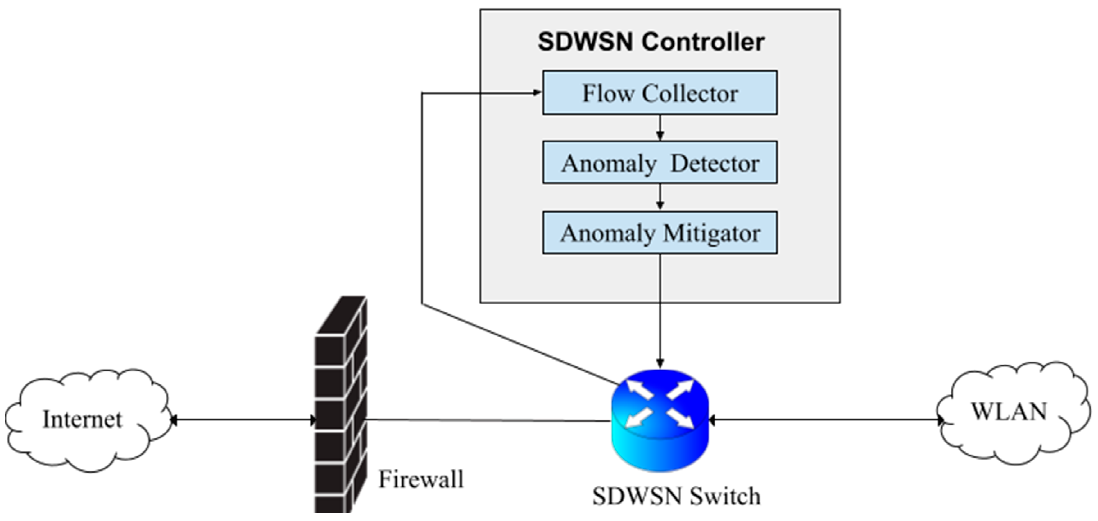
3.3. Anomaly Detectors
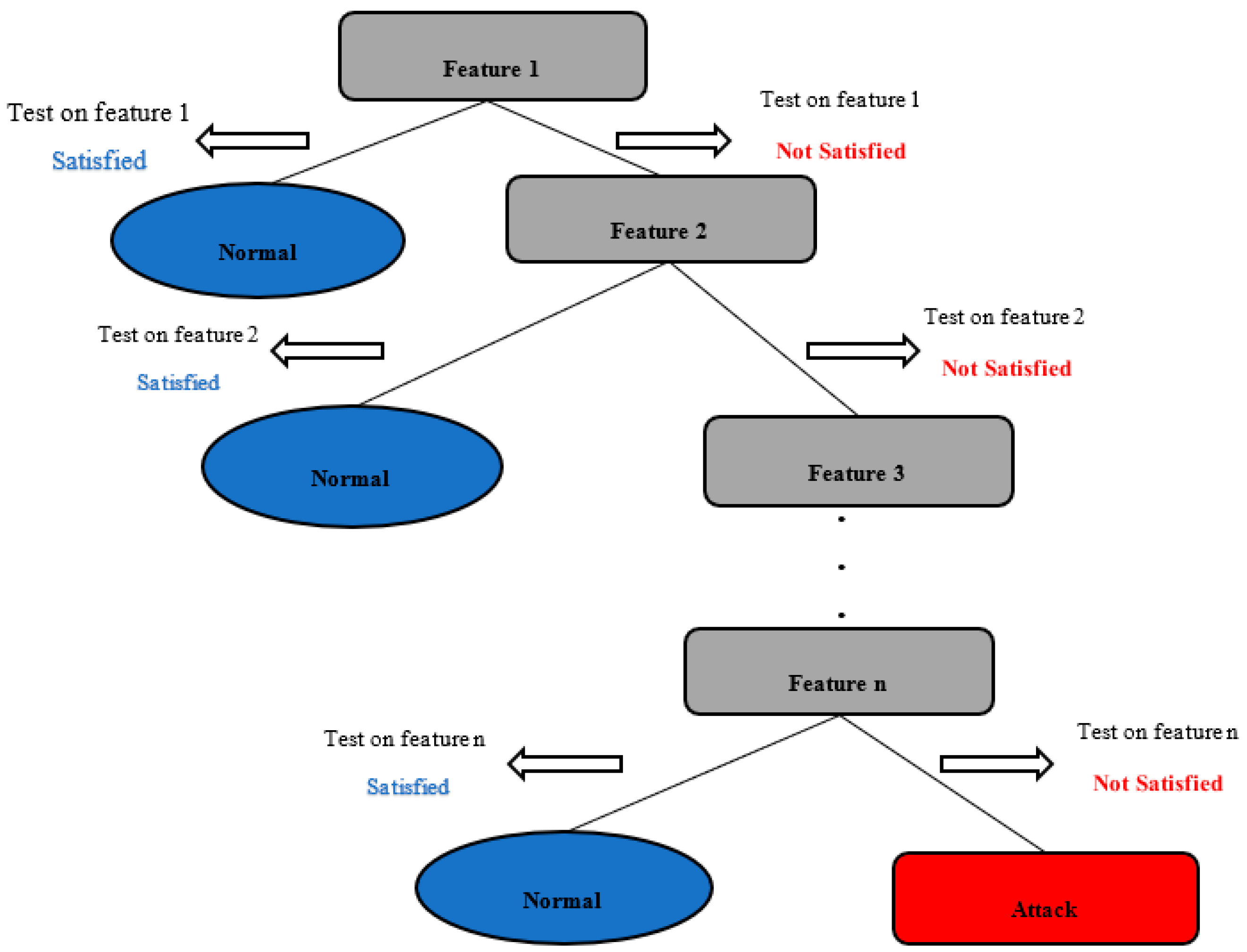
3.3.1. Decision Tree
- Allot the most important feature to the root of the tree
- Divide the training set into subsets having the same value for a feature
- Repeat the steps above until all the leaf nodes are found
- End the algorithm when all the leaf nodes are found.
3.3.2. Naïve Bayes
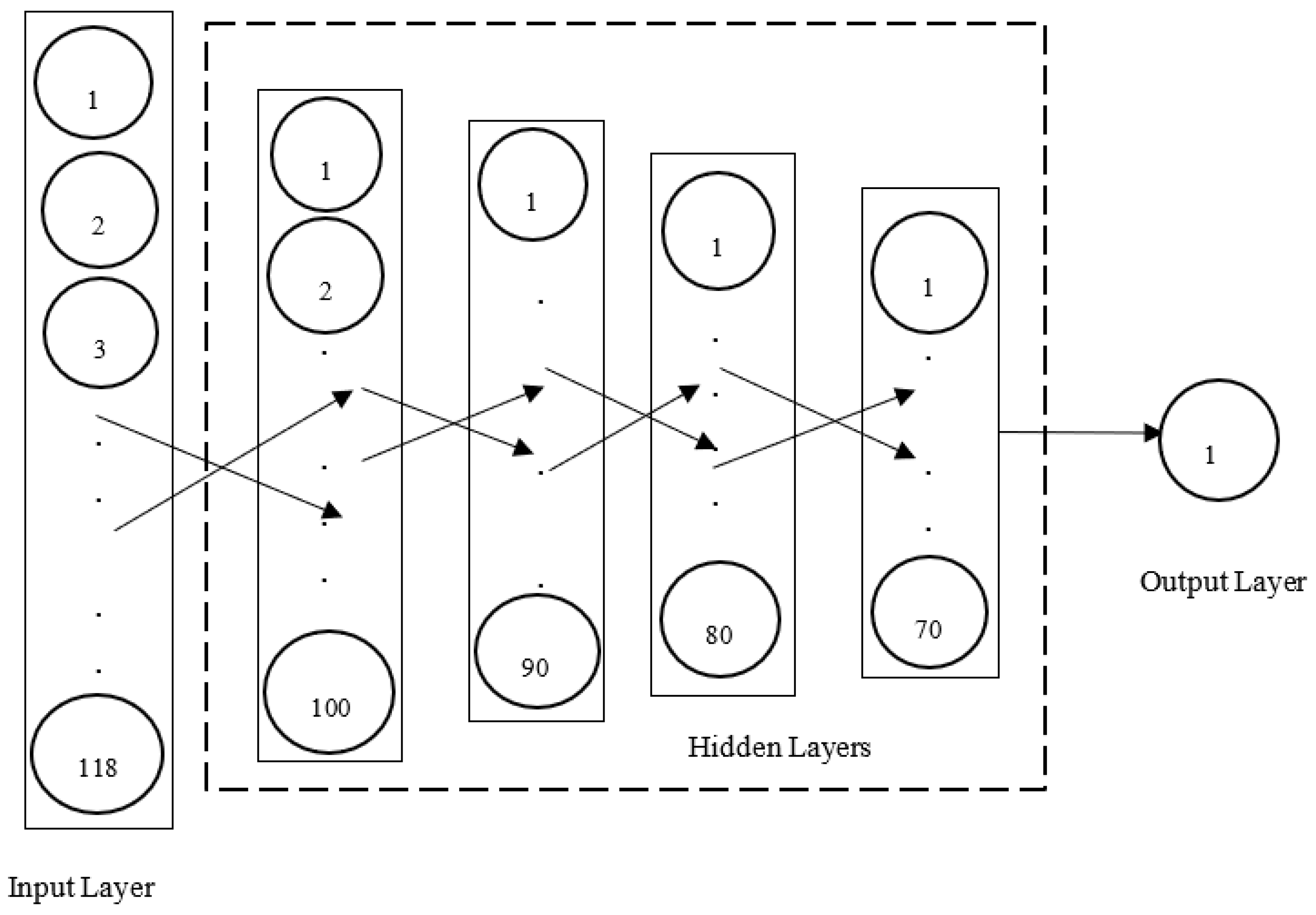
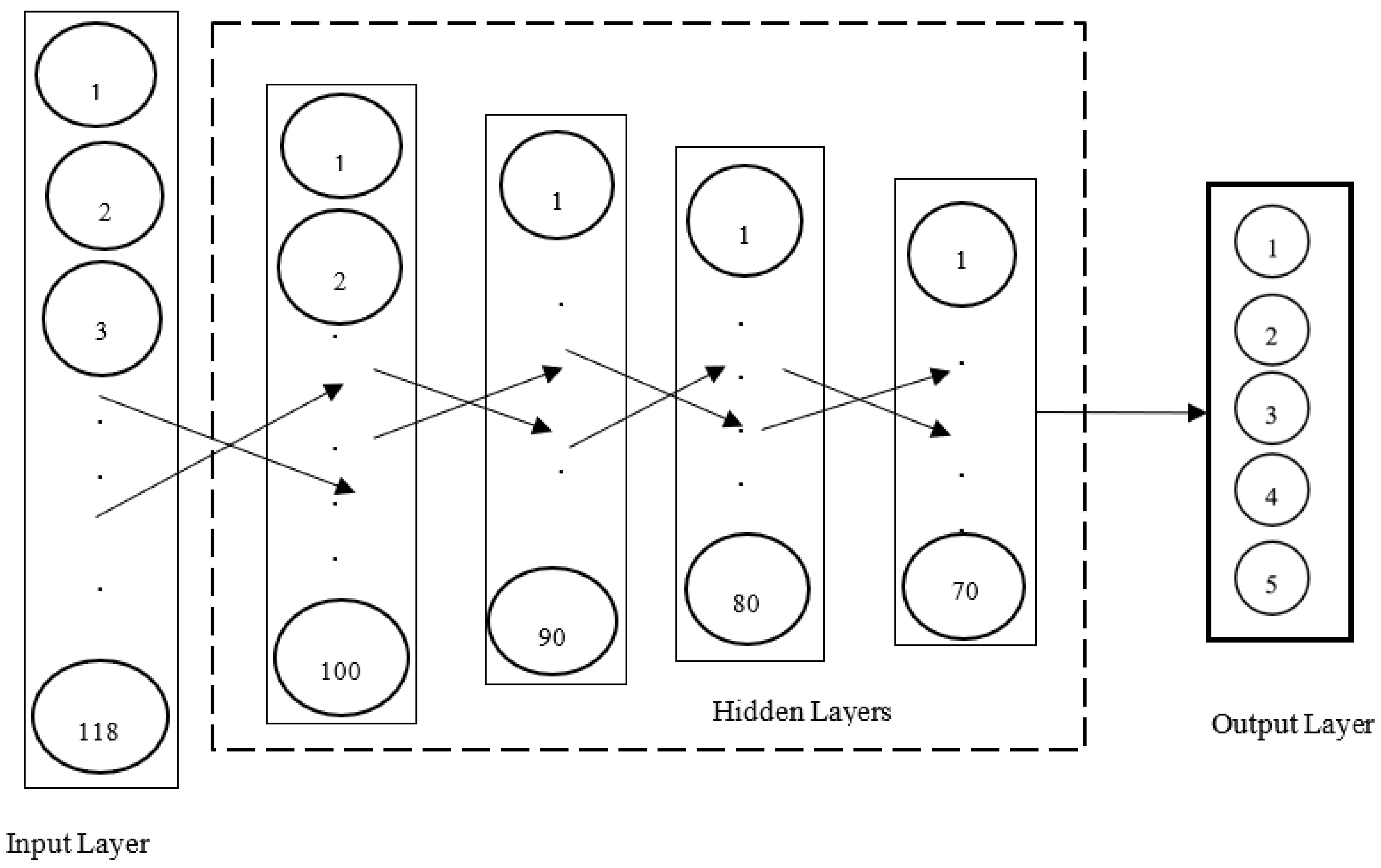
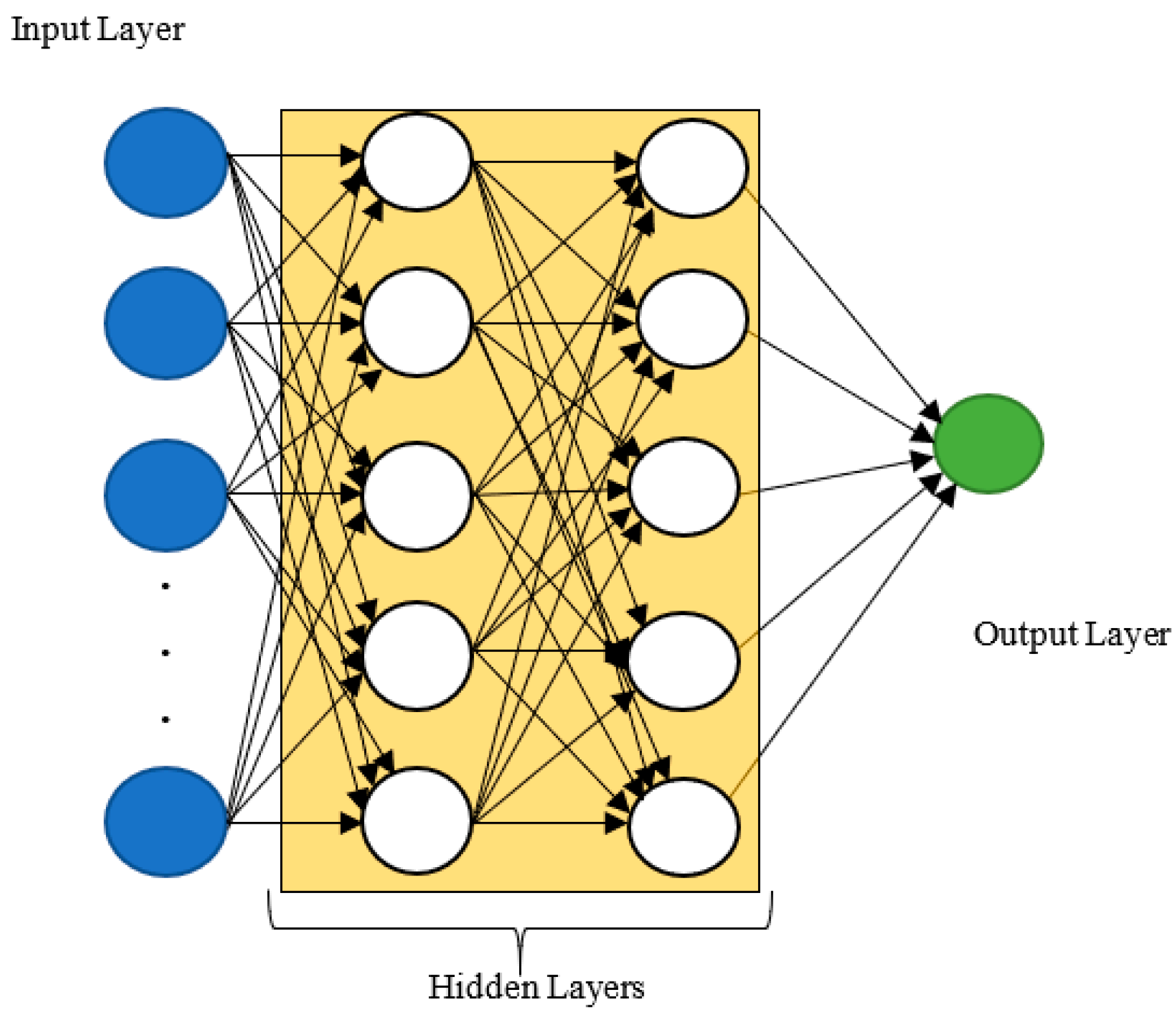
3.3.3. Deep Artificial Neural Network
- Using weights on every input value to a neuron. Where i = 1…m, and m is the number of input values;
- Computing the weighted sum of the input values to the neuron ;
- Adding a bias term to ;
- Using an activation function to introduce a non-linearity between the input values and the output value of the neuron.
- Initialize weights
- Calculate the cost function on the training samples
- Update the weights using the gradient descent approach
- Repeat the steps 2 and 3 until the chosen traditional performance metric does not improve anymore
4. Experimental Setup and Results
4.1. Binary Classification
4.1.1. NB-Based Anomaly Detector
4.1.2. DT-Based Anomaly Detector
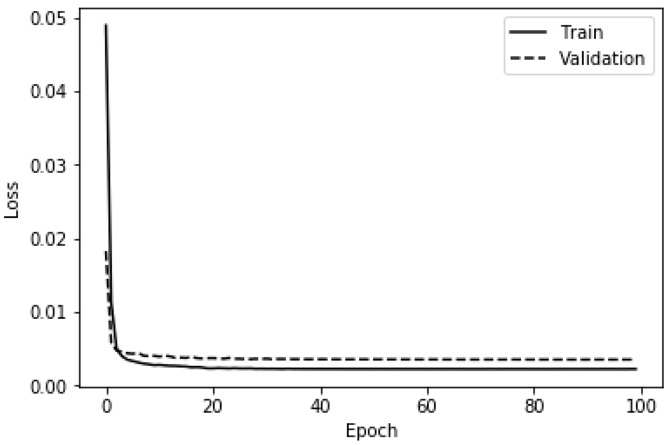
4.1.3. Deep ANN-Based Anomaly Detector
4.2. Multinomial Classification
4.2.1. NB-Based Anomaly Detector
4.2.2. DT-Based Anomaly Detector
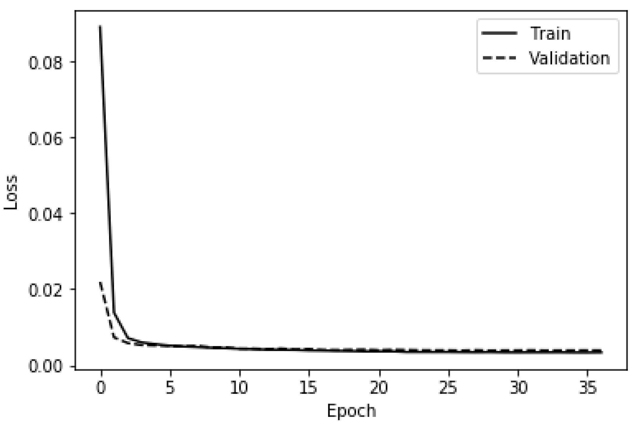
4.2.3. Deep ANN-Based Anomaly Detector
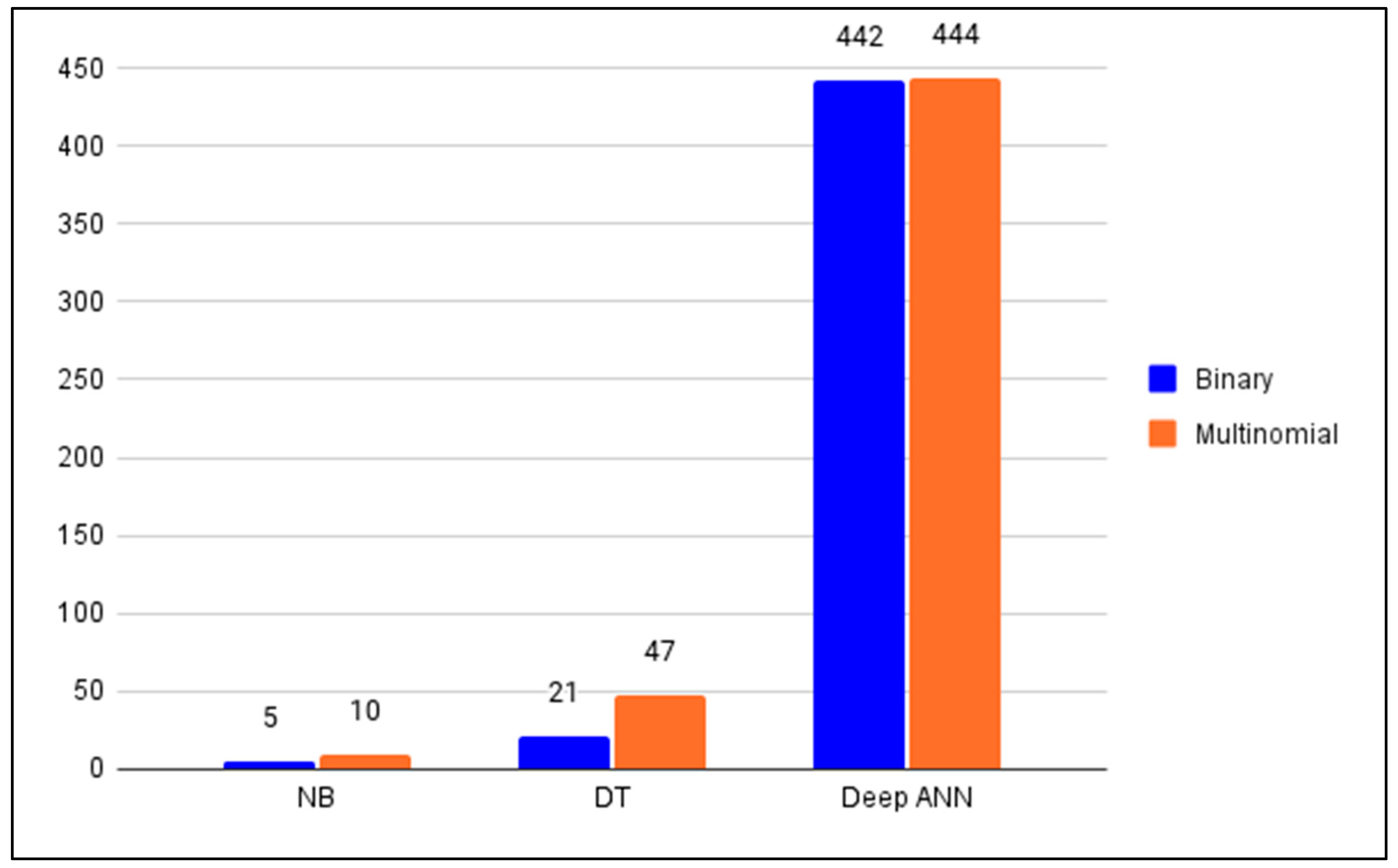
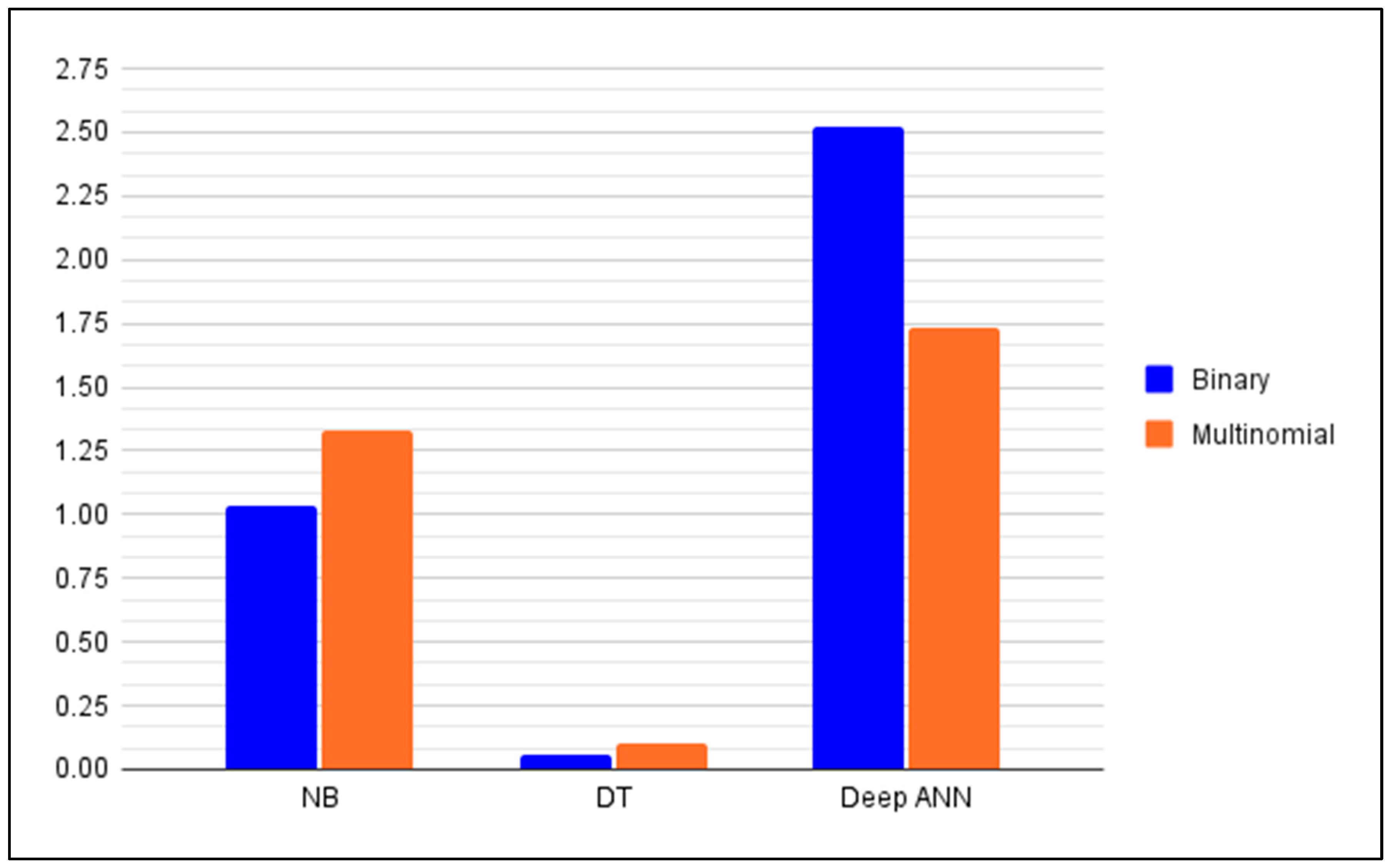
5. Summary and Discussion
6. Conclusions
Author Contributions
Funding
Institutional Review Board Statement
Informed Consent Statement
Data Availability Statement
Conflicts of Interest
Abbreviations
| Abbreviation | Meaning |
|---|---|
| ANN | Artificial Neural Network |
| DOS | Denial of Service |
| DT | Decision Tree |
| ELU | Exponential Linear Unit |
| FMIFS | Filter-based Mutual Information Feature Selection |
| FN | False Negative |
| FP | False Positive |
| h | Hours |
| IDS | Intrusion Detection System |
| IEEE | Institute of Electrical and Electronics Engineers |
| IoT | Internet of Things |
| kB | Kilobytes |
| LSSVM | Least Square Support Vector Machine |
| MAP | Maximum a Posteriori |
| min | Minutes |
| NB | Naïve Bayes |
| NSL-KDD | Network Security Laboratory-Knowledge Discovery in Databases |
| R2L | Remote to Local |
| ReLU | Rectified Linear Unit |
| s | Seconds |
| SDN | Software-Defined Network |
| SDWSN | Software-Defined Wireless Sensor Network |
| TN | True Negative |
| TP | True Positive |
| U2R | User to Root |
| WLAN | Wireless Local Area Network |
| WSN | Wireless Sensor Network |
References
- Gubbi, J.; Buyya, R.; Marusic, S.; Palaniswami, M. Internet of Things (IoT): A vision, architectural elements, and future directions. Future Gener. Comput. Syst. 2013, 29, 1645–1660. [Google Scholar] [CrossRef] [Green Version]
- Graf, B.; King, R.S.; Schiller, C.; Roessner, A. Development of an intelligent care cart and new supplies concepts for care homes and hospitals. In Proceedings of the ISR 2016: 47th International Symposium on Robotics, Munich, Germany, 21–22 June 2016; pp. 1–6. [Google Scholar]
- Basaklar, T.; Tuncel, Y.; An, S.; Ogras, U. Wearable Devices and Low-Power Design for Smart Health Applications: Challenges and Opportunities. In Proceedings of the 2021 IEEE/ACM International Symposium on Low Power Electronics and Design (ISLPED), Boston, MA, USA, 26–28 July 2021. [Google Scholar] [CrossRef]
- Iqbal, S.M.A.; Mahgoub, I.; Du, E.; Leavitt, M.A.; Asghar, W. Advances in healthcare wearable devices. NPJ Flex. Electron. 2021, 5, 9. [Google Scholar] [CrossRef]
- Topol, E.J. High-performance medicine: The convergence of human and artificial intelligence. Nat. Med. 2019, 25, 44–56. [Google Scholar] [CrossRef] [PubMed]
- Wu, F.; Qiu, C.; Wu, T.; Yuce, M.R. Edge-Based Hybrid System Implementation for Long-Range Safety and Healthcare IoT Applications. IEEE Internet Things J. 2021, 8, 9970–9980. [Google Scholar] [CrossRef]
- Pasluosta, C.F.; Gassner, H.; Winkler, J.; Klucken, J.; Eskofier, B.M. An Emerging Era in the Management of Parkinson’s Disease: Wearable Technologies and the Internet of Things. IEEE J. Biomed. Health Inform. 2015, 19, 1873–1881. [Google Scholar] [CrossRef] [PubMed]
- Kleinsasser, M.; Tharpe, B.; Akula, N.; Tirumani, H.; Sunderraman, R.; Bourgeois, A.G. Detecting and Predicting Sleep Activity using Biometric Sensor Data. In Proceedings of the 2022 14th International Conference on COMmunication Systems & NETworkS (COMSNETS), Bangalore, India, 4–8 January 2022; pp. 19–24. [Google Scholar]
- Kasinathan, P.; Pastrone, C.; Spirito, M.A.; Vinkovits, M. Denial-of-Service detection in 6LoWPAN based Internet of Things. In Proceedings of the 2013 IEEE 9th International Conference on Wireless and Mobile Computing, Networking and Communications (WiMob), Lyon, France, 25 November 2013; pp. 600–607. [Google Scholar]
- Kreutz, D.; Ramos, F.M.V.; Verissimo, P. Towards secure and dependable software-defined networks. In Proceedings of the Second ACM SIGCOMM Workshop on Hot Topics in Software Defined Networking, Hong Kong, China, 16 August 2013; pp. 55–60. [Google Scholar]
- Ndiaye, M.; Hancke, P.G.; Abu-Mahfouz, M.A. Software Defined Networking for Improved Wireless Sensor Network Management: A Survey. Sensors 2017, 17, 1031. [Google Scholar] [CrossRef] [PubMed]
- Nunes, B.A.A.; Mendonca, M.; Nguyen, X.; Obraczka, K.; Turletti, T. A Survey of Software-Defined Networking: Past, Present, and Future of Programmable Networks. IEEE Commun. Surv. Tutor. 2014, 16, 1617–1634. [Google Scholar] [CrossRef] [Green Version]
- Kobo, H.I.; Abu-Mahfouz, A.M.; Hancke, G.P. A Survey on Software-Defined Wireless Sensor Networks: Challenges and Design Requirements. IEEE Access 2017, 5, 1872–1899. [Google Scholar] [CrossRef]
- Akyildiz, I.F.; Su, W.; Sankarasubramaniam, Y.; Cayirci, E. A survey on sensor networks. IEEE Commun. Mag. 2002, 40, 102–114. [Google Scholar] [CrossRef] [Green Version]
- Liu, A.; Ning, P. TinyECC: A configurable library for elliptic curve cryptography in wireless sensor networks. In Proceedings of the 7th International Conference on Information Processing in Sensor Networks, St. Louis, MO, USA, 2 May 2008; pp. 245–256. [Google Scholar]
- Kobo, H.I.; Abu-Mahfouz, A.M.; Hancke, G.P. Efficient controller placement and reelection mechanism in distributed control system for software defined wireless sensor networks. Trans. Emerg. Telecommun. Technol. 2019, 30, e3588. [Google Scholar] [CrossRef]
- Dolev, S.; David, S.T. SDN-based private interconnection. In Proceedings of the 2014 IEEE 13th International Symposium on Network Computing and Applications, Cambridge, MA, USA, 21–23 August 2014; pp. 129–136. [Google Scholar]
- Choi, Y.; Lee, D.; Kim, J.; Jung, J.; Nam, J.; Won, D. Security enhanced user authentication protocol for wireless sensor networks using elliptic curves cryptography. Sensors 2014, 14, 10081–10106. [Google Scholar] [CrossRef] [PubMed] [Green Version]
- Lounis, A.; Hadjidj, A.; Bouabdallah, A.; Challal, Y. Secure and scalable cloud-based architecture for e-health wireless sensor networks. In Proceedings of the 2012 21st International Conference on Computer Communications and Networks (ICCCN), Munich, Germany, 31 August 2012; pp. 1–7. [Google Scholar]
- Forouzan, B.A. Cryptography & Network Security; McGraw-Hill, Inc.: New York, NY, USA, 2007. [Google Scholar]
- Hoffstein, J.; Pipher, J.; Silverman, J.H.; Silverman, J.H. An Introduction to Mathematical Cryptography; Springer: Berlin/Heidelberg, Germany, 2008; Volume 1. [Google Scholar]
- Rajasegarar, S.; Leckie, C.; Palaniswami, M. Anomaly detection in wireless sensor networks. IEEE Wirel. Commun. 2008, 15, 34–40. [Google Scholar] [CrossRef]
- Gogoi, P.; Bhuyan, M.H.; Bhattacharyya, D.; Kalita, J.K. Packet and flow based network intrusion dataset. In Proceedings of the International Conference on Contemporary Computing, Noida, India, 6–8 August 2012; pp. 322–334. [Google Scholar]
- Hodo, E.; Bellekens, X.; Hamilton, A.; Dubouilh, P.-L.; Iorkyase, E.; Tachtatzis, C.; Atkinson, R. Threat analysis of IoT networks using artificial neural network intrusion detection system. In Proceedings of the 2016 International Symposium on Networks, Computers and Communications (ISNCC), Yasmine Hammamet, Tunisia, 17 November 2016; pp. 1–6. [Google Scholar]
- Gope, P.; Hwang, T. BSN-Care: A Secure IoT-Based Modern Healthcare System Using Body Sensor Network. IEEE Sens. J. 2016, 16, 1368–1376. [Google Scholar] [CrossRef]
- Min, M.; Wan, X.; Xiao, L.; Chen, Y.; Xia, M.; Wu, D.; Dai, H. Learning-Based Privacy-Aware Offloading for Healthcare IoT With Energy Harvesting. IEEE Internet Things J. 2019, 6, 4307–4316. [Google Scholar] [CrossRef]
- Tang, T.A.; Mhamdi, L.; McLernon, D.; Zaidi, S.A.R.; Ghogho, M. Deep learning approach for Network Intrusion Detection in Software Defined Networking. In Proceedings of the 2016 International Conference on Wireless Networks and Mobile Communications (WINCOM), Fez, Morocco, 26–29 October 2016; pp. 258–263. [Google Scholar]
- Umba, S.M.W.; Abu-Mahfouz, A.M.; Ramotsoela, T.D.; Hancke, G.P. A Review of Artificial Intelligence Based Intrusion Detection for Software-Defined Wireless Sensor Networks. In Proceedings of the 2019 IEEE 28th International Symposium on Industrial Electronics (ISIE), Vancouver, BC, Canada, 12–14 June 2019; pp. 1277–1282. [Google Scholar]
- Umba, S.M.W.; Abu-Mahfouz, A.M.; Ramotsoela, T.D.; Hancke, G.P. Comparative Study of Artificial Intelligence Based Intrusion Detection for Software-Defined Wireless Sensor Networks. In Proceedings of the 2019 IEEE 28th International Symposium on Industrial Electronics (ISIE), Vancouver, BC, Canada, 12–14 June 2019; pp. 2220–2225. [Google Scholar]
- Sperotto, A.; Schaffrath, G.; Sadre, R.; Morariu, C.; Pras, A.; Stiller, B. An overview of IP flow-based intrusion detection. IEEE Commun. Surv. Tutor. 2010, 12, 343–356. [Google Scholar] [CrossRef] [Green Version]
- Giotis, K.; Argyropoulos, C.; Androulidakis, G.; Kalogeras, D.; Maglaris, V. Combining OpenFlow and sFlow for an effective and scalable anomaly detection and mitigation mechanism on SDN environments. Comput. Netw. 2014, 62, 122–136. [Google Scholar] [CrossRef]
- Boero, L.; Marchese, M.; Zappatore, S. Support Vector Machine Meets Software Defined Networking in IDS Domain. In Proceedings of the 2017 29th International Teletraffic Congress (ITC 29), Genoa, Italy, 4–8 September 2017; pp. 25–30. [Google Scholar]
- Panda, M.; Patra, M.R. Network intrusion detection using naive bayes. Int. J. Comput. Sci. Netw. Secur. 2007, 7, 258–263. [Google Scholar]
- MeeraGandhi, G.; Appavoo, K.; Srivasta, S. Effective network intrusion detection using classifiers decision trees and decision rules. Int. J. Adv. Netw. Appl. 2010, 686–692. [Google Scholar]
- Ioannis, K.; Dimitriou, T.; Freiling, F.C. Towards intrusion detection in wireless sensor networks. In Proceedings of the 13th European Wireless Conference, Paris, France, 1–4 April 2007; pp. 1–10. [Google Scholar]
- Ambusaidi, M.A.; He, X.; Nanda, P.; Tan, Z. Building an Intrusion Detection System Using a Filter-Based Feature Selection Algorithm. IEEE Trans. Comput. 2016, 65, 2986–2998. [Google Scholar] [CrossRef] [Green Version]
- Ryan, J.; Lin, M.-J.; Miikkulainen, R. Intrusion detection with neural networks. In Proceeding of the 1997 Conference on Advances in Neural Information Processing Systems, Denver, CO, USA, 1–6 December 1997; pp. 943–949. [Google Scholar]
- Shariati, M.; Mafipour, M.S.; Mehrabi, P.; Shariati, A.; Toghroli, A.; Trung, N.T.; Salih, M.N.A. A novel approach to predict shear strength of tilted angle connectors using artificial intelligence techniques. Eng. Comput. 2021, 37, 2089–2109. [Google Scholar] [CrossRef]
- Daniels, J.; Herrero, P.; Georgiou, P. A Deep Learning Framework for Automatic Meal Detection and Estimation in Artificial Pancreas Systems. Sensors 2022, 22, 466. [Google Scholar] [CrossRef] [PubMed]
- Braune, K.; Lal, R.A.; Petruželková, L.; Scheiner, G.; Winterdijk, P.; Schmidt, S.; Raimond, L.; Hood, K.K.; Riddell, M.C.; Skinner, T.C.; et al. Open-source automated insulin delivery: International consensus statement and practical guidance for health-care professionals. Lancet Diabetes Endocrinol. 2022, 10, 58–74. [Google Scholar] [CrossRef]
- Hu, F.; Hao, Q.; Bao, K. A survey on software-defined network and openflow: From concept to implementation. IEEE Commun. Surv. Tutor. 2014, 16, 2181–2206. [Google Scholar] [CrossRef]
- Ramotsoela, D.; Abu-Mahfouz, A.; Hancke, G.P. A Survey of Anomaly Detection in Industrial Wireless Sensor Networks with Critical Water System Infrastructure as a Case Study; MDPI: Basel, Switzerland, 2018; Volume 2018. [Google Scholar] [CrossRef] [Green Version]
- Åkerberg, J.; Gidlund, M.; Björkman, M. Future research challenges in wireless sensor and actuator networks targeting industrial automation. In Proceedings of the 2011 9th IEEE International Conference on Industrial Informatics, Lisbon, Portugal, 6 October 2011; pp. 410–415. [Google Scholar]
- Kumar, M.; Cohen, K.; HomChaudhuri, B. Cooperative Control of Multiple Uninhabited Aerial Vehicles for Monitoring and Fighting Wildfires. J. Aerosp. Comput. Inf. Commun. 2011, 8, 1–16. [Google Scholar] [CrossRef]
- KDD Dataset 1999. Available online: http://kdd.ics.uci.edu/databases/kddcup99/ (accessed on 15 October 2019).
- Tavallaee, M.; Bagheri, E.; Lu, W.; Ghorbani, A.A. A detailed analysis of the KDD CUP 99 data set. In Proceedings of the Symposium on Computational Intelligence for Security and Defense Applications, Ottawa, ON, Canada, 8–10 July 2009; pp. 1–6. [Google Scholar]
- Shalev-Shwartz, S.; Ben-David, S. Understanding Machine Learning: From Theory to Algorithms; Cambridge University Press: Cambridge, UK, 2014; p. 424. [Google Scholar]
- Goutte, C.; Gaussier, E. A probabilistic interpretation of precision, recall and F-score, with implication for evaluation. In Proceedings of the European Conference on Information Retrieval, Santiago de Compostela, Spain, 21–23 March 2005; pp. 345–359. [Google Scholar]
- Raymond, D.R.; Midkiff, S.F. Denial-of-service in wireless sensor networks: Attacks and defenses. IEEE Pervasive Comput. 2008, 7, 74–81. [Google Scholar] [CrossRef]
- Ren, K.; Yu, S.; Lou, W.; Zhang, Y. Multi-user broadcast authentication in wireless sensor networks. IEEE Trans. Veh. Technol. 2009, 58, 4554–4564. [Google Scholar] [CrossRef]
- Pongle, P.; Chavan, G. A survey: Attacks on RPL and 6LoWPAN in IoT. In Proceedings of the 2015 International conference on pervasive computing (ICPC), Pune, India, 8–10 January 2015; pp. 1–6. [Google Scholar]
- Liu, Y.; Ma, M.; Liu, X.; Xiong, N.; Liu, A.; Zhu, Y. Design and analysis of probing route to defense sink-hole attacks for Internet of Things security. IEEE Trans. Netw. Sci. Eng. 2018, 7, 356–372. [Google Scholar] [CrossRef]
- Butun, I.; Morgera, S.D.; Sankar, R. A survey of intrusion detection systems in wireless sensor networks. IEEE Commun. Surv. Tutor. 2013, 16, 266–282. [Google Scholar] [CrossRef]
- Lee, C.; Lee, G.G. Information gain and divergence-based feature selection for machine learning-based text categorization. Inf. Process. Manag. 2006, 42, 155–165. [Google Scholar] [CrossRef]
- Uğuz, H. A two-stage feature selection method for text categorization by using information gain, principal component analysis and genetic algorithm. Knowl.-Based Syst. 2011, 24, 1024–1032. [Google Scholar] [CrossRef]
- Zhang, C.; Vinyals, O.; Munos, R.; Bengio, S. A study on overfitting in deep reinforcement learning. arXiv 2018, arXiv:1804.06893. [Google Scholar]
- Dietterich, T. Overfitting and undercomputing in machine learning. ACM Comput. Surv. (CSUR) 1995, 27, 326–327. [Google Scholar] [CrossRef]
- Mingers, J. An empirical comparison of pruning methods for decision tree induction. Mach. Learn. 1989, 4, 227–243. [Google Scholar] [CrossRef] [Green Version]
- Bradford, J.P.; Kunz, C.; Kohavi, R.; Brunk, C.; Brodley, C.E. Pruning decision trees with misclassification costs. In Proceedings of the European Conference on Machine Learning, Chemnitz, Germany, 21–23 April 1998; pp. 131–136. [Google Scholar]
- Goodfellow, I.; Bengio, Y.; Courville, A.; Bengio, Y. Deep Learning; MIT Press Cambridge: Cambridge, MA, USA, 2016; Volume 1. [Google Scholar]
- Gnedenko, B.V. Theory of Probability; Routledge: Oxfordshire, UK, 2018. [Google Scholar]
- DeGroot, M.H.; Schervish, M.J. Probability and Statistics; Pearson Education, Inc.: Boston, MA, USA, 2012. [Google Scholar]
- Deisenroth, M.P.; Faisal, A.A.; Ong, C.S. Mathematics for Machine Learning; Cambridge University Press: Cambridge, UK, 2020. [Google Scholar]
- Souza, C.R. Kernel functions for machine learning applications. Creat. Commons Attrib.-Noncommer.-Share Alike 2010, 3, 29. [Google Scholar]
- Ramachandran, P.; Zoph, B.; Le, Q.V. Searching for activation functions. arXiv 2017, arXiv:1710.05941. [Google Scholar]
- Han, J.; Moraga, C. The influence of the sigmoid function parameters on the speed of backpropagation learning. In Proceedings of the International Workshop on Artificial Neural Networks, Malaga-Torremolinos, Spain, 7–9 June 1995; pp. 195–201. [Google Scholar]
- Duan, K.; Keerthi, S.S.; Chu, W.; Shevade, S.K.; Poo, A.N. Multi-category classification by soft-max combination of binary classifiers. In Proceedings of the International Workshop on Multiple Classifier Systems, Guildford, UK, 11–13 June 2003; pp. 125–134. [Google Scholar]
- Collobert, R.; Bengio, S.; Mariéthoz, J. Torch: A Modular Machine Learning Software Library; Idiap: Martigny, Switzerland, 2002. [Google Scholar]
- Xu, B.; Wang, N.; Chen, T.; Li, M. Empirical evaluation of rectified activations in convolutional network. arXiv 2015, arXiv:1505.00853. [Google Scholar]
- Clevert, D.-A.; Unterthiner, T.; Hochreiter, S. Fast and accurate deep network learning by exponential linear units (elus). arXiv 2015, arXiv:1511.07289. [Google Scholar]
- Bengio, Y.; Simard, P.; Frasconi, P. Learning long-term dependencies with gradient descent is difficult. IEEE Trans. Neural Netw. 1994, 5, 157–166. [Google Scholar] [CrossRef] [PubMed]
- Ng, A. Machine Learning Yearning, 2016; Stanford University Press: Redwood City, CA, USA, 2017. [Google Scholar]
- Schmidhuber, J. Deep learning in neural networks: An overview. Neural Netw. 2015, 61, 85–117. [Google Scholar] [CrossRef] [PubMed] [Green Version]
- Ruder, S. An overview of gradient descent optimization algorithms. arXiv 2016, arXiv:1609.04747. [Google Scholar]
- Bottou, L. Stochastic gradient descent tricks. In Neural Networks: Tricks of the Trade; Springer: Berlin/Heidelberg, Germany, 2012; pp. 421–436. [Google Scholar]
- Rumelhart, D.E.; Hinton, G.E.; Williams, R.J. Learning representations by back-propagating errors. Nature 1986, 323, 533–536. [Google Scholar] [CrossRef]
- Hertz, J.A. Introduction to the Theory of Neural Computation; CRC Press: Boca Raton, FL, USA, 2018. [Google Scholar]
- Forman, G. An extensive empirical study of feature selection metrics for text classification. J. Mach. Learn. Res. 2003, 3, 1289–1305. [Google Scholar]
- Karabulut, E.M.; Özel, S.A.; Ibrikci, T. A comparative study on the effect of feature selection on classification accuracy. Procedia Technol. 2012, 1, 323–327. [Google Scholar] [CrossRef] [Green Version]
- Kdd-Cup-99-Analysis-Machine-Learning-Python. Available online: https://github.com/chadlimedamine/kdd-cup-99-Analysis-machine-learning-python (accessed on 21 November 2019).
- Haury, A.-C.; Gestraud, P.; Vert, J.-P. The influence of feature selection methods on accuracy, stability and interpretability of molecular signatures. PLoS ONE 2011, 6, e28210. [Google Scholar] [CrossRef] [PubMed]
- Wang, W.; Zhang, X.; Gombault, S.; Knapskog, S.J. Attribute normalization in network intrusion detection. In Proceedings of the 2009 10th International Symposium on Pervasive Systems, Algorithms, and Networks, Kaoshiung, Taiwan, 14–16 December 2009; pp. 448–453. [Google Scholar]
- Chan, T.F.; Golub, G.H.; LeVeque, R.J. Updating formulae and a pairwise algorithm for computing sample variances. In Proceedings of the COMPSTAT 1982 5th Symposium, Toulouse, France, 1 January 1982; pp. 30–41. [Google Scholar]
- Sklearn. Available online: https://scikit-learn.org/stable/ (accessed on 23 November 2019).
- Chollet, F. Deep Learning with Python; Manning Publications Co.: Shelter Island, NY, USA, 2017; p. 384. [Google Scholar]
- Kolosnjaji, B.; Zarras, A.; Webster, G.; Eckert, C. Deep learning for classification of malware system call sequences. In Proceedings of the Australasian Joint Conference on Artificial Intelligence, Hobart, Australia, 5–8 December 2016; pp. 137–149. [Google Scholar]
- Zhang, C.; Bengio, S.; Hardt, M.; Recht, B.; Vinyals, O. Understanding deep learning requires rethinking generalization. arXiv 2016, arXiv:1611.03530. [Google Scholar] [CrossRef]
- Ugwuanyi, S.; Paul, G.; Irvine, J. Survey of IoT for Developing Countries: Performance Analysis of LoRaWAN and Cellular NB-IoT Networks. Electronics 2021, 10, 2224. [Google Scholar] [CrossRef]
- Alippi, C.; Anastasi, G.; Di Francesco, M.; Roveri, M. Energy management in wireless sensor networks with energy-hungry sensors. IEEE Instrum. Meas. Mag. 2009, 12, 16–23. [Google Scholar] [CrossRef]
- Gong, D.; Yang, Y. Low-latency SINR-based data gathering in wireless sensor networks. IEEE Trans. Wirel. Commun. 2014, 13, 3207–3221. [Google Scholar] [CrossRef]
- Kraft, D.; Srinivasan, K.; Bieber, G. Deep Learning Based Fall Detection Algorithms for Embedded Systems, Smartwatches, and IoT Devices Using Accelerometers. Technologies 2020, 8, 72. [Google Scholar] [CrossRef]
- Wei, J.; Wang, Z.; Xing, X. A Wireless High-Sensitivity Fetal Heart Sound Monitoring System. Sensors 2021, 21, 193. [Google Scholar] [CrossRef]
- Kubat, M.; Matwin, S. Addressing the curse of imbalanced training sets: One-sided selection. In Proceedings of the 14th International Conference on Machine Learning, San Francisco, CA, USA, 8–12 July 1997; pp. 179–186. [Google Scholar]
- Maratea, A.; Petrosino, A.; Manzo, M. Adjusted F-measure and kernel scaling for imbalanced data learning. Inf. Sci. 2014, 257, 331–341. [Google Scholar] [CrossRef]
- Taylor, L.; Nitschke, G. Improving deep learning using generic data augmentation. arXiv 2017, arXiv:1708.06020. [Google Scholar]
- Cubuk, E.D.; Zoph, B.; Mane, D.; Vasudevan, V.; Le, Q.V. Autoaugment: Learning augmentation strategies from data. In Proceedings of the IEEE Conference on Computer Vision and Pattern Recognition, Long Beach, CA, USA, 15–20 June 2019; pp. 113–123. [Google Scholar]
- Wang, F.; Wang, D.; Liu, J. Traffic-aware relay node deployment: Maximizing lifetime for data collection wireless sensor networks. IEEE Trans. Parallel Distrib. Syst. 2011, 22, 1415–1423. [Google Scholar] [CrossRef] [Green Version]


| Metric | Symbol | Formula |
|---|---|---|
| Accuracy | Ac | |
| Precision | P | |
| Recall | R | |
| F-score | F |
| Traffics | Training | Test | |
|---|---|---|---|
| Normal | 67,343 | 9711 | |
| Attacks | DoS | 45,927 | 7458 |
| U2R | 52 | 67 | |
| R2L | 995 | 2887 | |
| Probing | 11,656 | 2421 | |
| Metric | NB-Based | DT-Based |
|---|---|---|
| Accuracy | 0.948038 | 0.999777 |
| Precision | 0.999114 | 0.999285 |
| Recall | 0.792679 | 0.999591 |
| F-score | 0.884005 | 0.999438 |
| Prediction time | 1.034252 s | 0.059382 s |
| Run time | 32.054979 s | 26.814881 s |
| Memory size | 5 kB | 21 kB |
| Learning Rate | Accuracy | Precision | Recall | F-Score |
|---|---|---|---|---|
| 0.1 | 0.196240 | 1.000000 | 0.196240 | 0.328095 |
| 0.001 | 0.999021 | 0.998177 | 0.996840 | 0.997508 |
| 0.00001 | 0.999433 | 0.998830 | 0.997973 | 0.998401 |
| Metric | Value |
|---|---|
| Accuracy | 0.999433 |
| Precision | 0.998830 |
| Recall | 0.997973 |
| F-score | 0.998401 |
| Prediction time | 2.520133 s |
| Run time | 2 h 20 min 23.361987 s |
| Memory size | 442 kB |
| Class | Precision | Recall | F-Score |
|---|---|---|---|
| Normal | 1.00 | 0.72 | 0.84 |
| DoS | 0.04 | 0.94 | 0.07 |
| U2R | 0.23 | 0.43 | 0.30 |
| R2L | 0.01 | 1.00 | 0.01 |
| Probing | 0.97 | 0.91 | 0.94 |
| Metric | Value |
|---|---|
| Prediction time | 1.334464 s |
| Run time | 15.390072 s |
| Memory size | 10 kB |
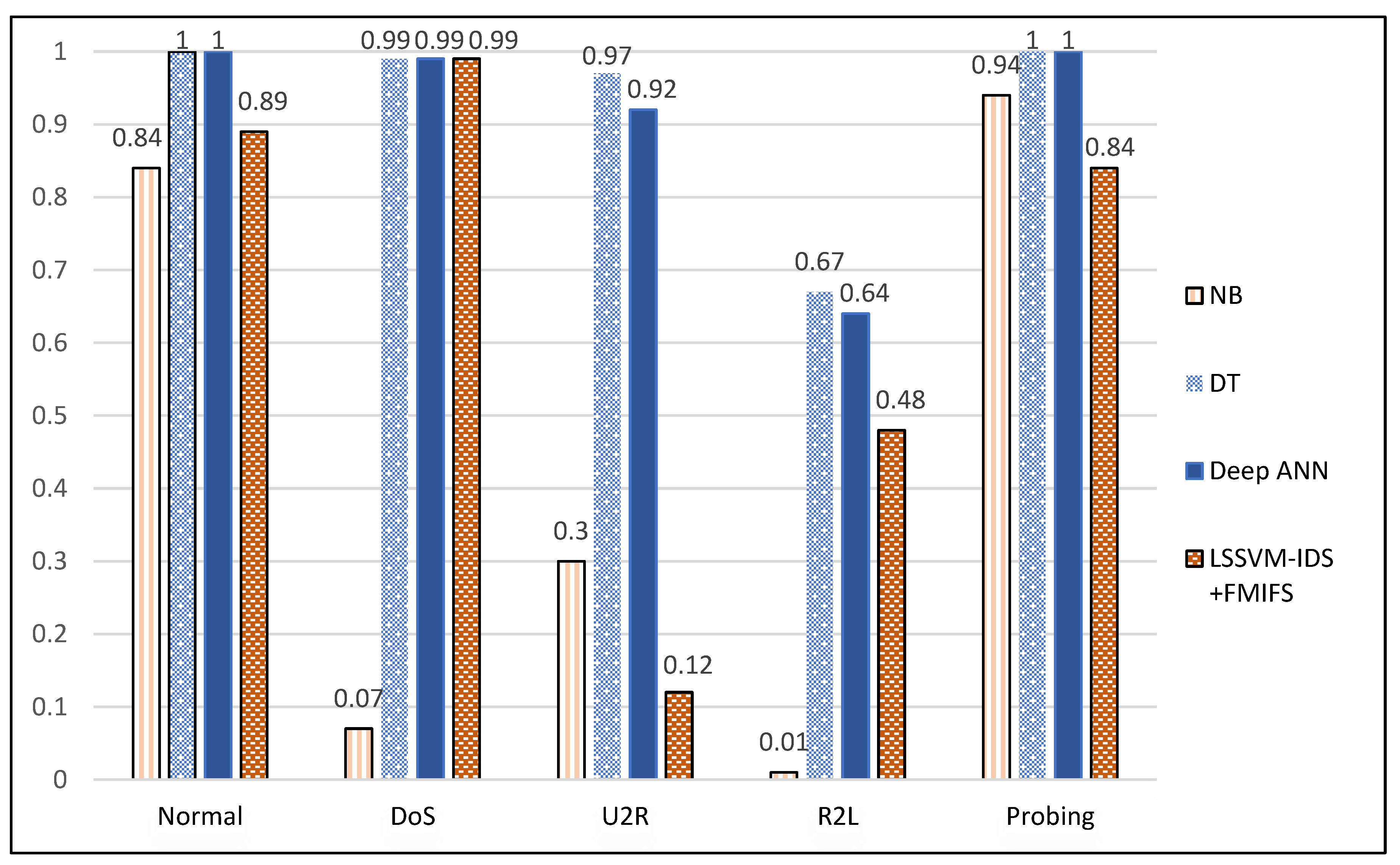
| Class | Precision | Recall | F-Score |
|---|---|---|---|
| Normal | 1.00 | 1.00 | 1.00 |
| DoS | 0.99 | 0.99 | 0.99 |
| U2R | 0.96 | 0.98 | 0.97 |
| R2L | 0.67 | 0.67 | 0.67 |
| Probing | 1.00 | 1.00 | 1.00 |
| Metric | Value |
|---|---|
| Prediction time | 0.106718 s |
| Run time | 19.176359 s |
| Memory size | 47 kB |
| Class | Precision | Recall | F-Score |
|---|---|---|---|
| Normal | 1.00 | 1.00 | 1.00 |
| DoS | 0.99 | 0.98 | 0.99 |
| U2R | 0.94 | 0.90 | 0.92 |
| R2L | 1.00 | 0.47 | 0.64 |
| Probing | 1.00 | 1.00 | 1.00 |
| Metric | Value |
|---|---|
| Prediction time | 1.729457 s |
| Run time | 53 min 23.449426 s |
| Memory size | 444 kB |
| Metric | NB | DT | Deep ANN |
|---|---|---|---|
| Accuracy | 0.948038 | 0.999777 | 0.999433 |
| Precision | 0.999114 | 0.999285 | 0.998830 |
| Recall | 0.792679 | 0.999591 | 0.997973 |
| F-score | 0.884005 | 0.999438 | 0.998401 |
| Prediction time | 1.034252 s | 0.059382 s | 2.520133 s |
| Run time | 32.054979 s | 26.814881 s | 2 h 20 min 23.361987 s |
| Memory size | 5 kB | 21 kB | 442 kB |
| SDWSN Requirements | NB | DT | Deep ANN |
|---|---|---|---|
| High level of security required | NO | YES | YES |
| Low memory capacity | YES | YES | NO |
| High performance required (i.e., low latency) | YES | YES | YES |
| SDWSN Requirements | NB | DT | Deep ANN |
|---|---|---|---|
| High level of security required | NO | YES | YES |
| Low memory capacity | NO | YES | NO |
| High performance required (i.e., low latency) | NO | YES | YES |
| High Level of Security Required | Low Memory Capacity | High Performance Required (i.e., Low Latency) |
|---|---|---|
|
|
|
Publisher’s Note: MDPI stays neutral with regard to jurisdictional claims in published maps and institutional affiliations. |
© 2022 by the authors. Licensee MDPI, Basel, Switzerland. This article is an open access article distributed under the terms and conditions of the Creative Commons Attribution (CC BY) license (https://creativecommons.org/licenses/by/4.0/).
Share and Cite
Masengo Wa Umba, S.; Abu-Mahfouz, A.M.; Ramotsoela, D. Artificial Intelligence-Driven Intrusion Detection in Software-Defined Wireless Sensor Networks: Towards Secure IoT-Enabled Healthcare Systems. Int. J. Environ. Res. Public Health 2022, 19, 5367. https://doi.org/10.3390/ijerph19095367
Masengo Wa Umba S, Abu-Mahfouz AM, Ramotsoela D. Artificial Intelligence-Driven Intrusion Detection in Software-Defined Wireless Sensor Networks: Towards Secure IoT-Enabled Healthcare Systems. International Journal of Environmental Research and Public Health. 2022; 19(9):5367. https://doi.org/10.3390/ijerph19095367
Chicago/Turabian StyleMasengo Wa Umba, Shimbi, Adnan M. Abu-Mahfouz, and Daniel Ramotsoela. 2022. "Artificial Intelligence-Driven Intrusion Detection in Software-Defined Wireless Sensor Networks: Towards Secure IoT-Enabled Healthcare Systems" International Journal of Environmental Research and Public Health 19, no. 9: 5367. https://doi.org/10.3390/ijerph19095367
APA StyleMasengo Wa Umba, S., Abu-Mahfouz, A. M., & Ramotsoela, D. (2022). Artificial Intelligence-Driven Intrusion Detection in Software-Defined Wireless Sensor Networks: Towards Secure IoT-Enabled Healthcare Systems. International Journal of Environmental Research and Public Health, 19(9), 5367. https://doi.org/10.3390/ijerph19095367