
Evaluating Changes in Health Risk from Drought over the Contiguous United States


Abstract
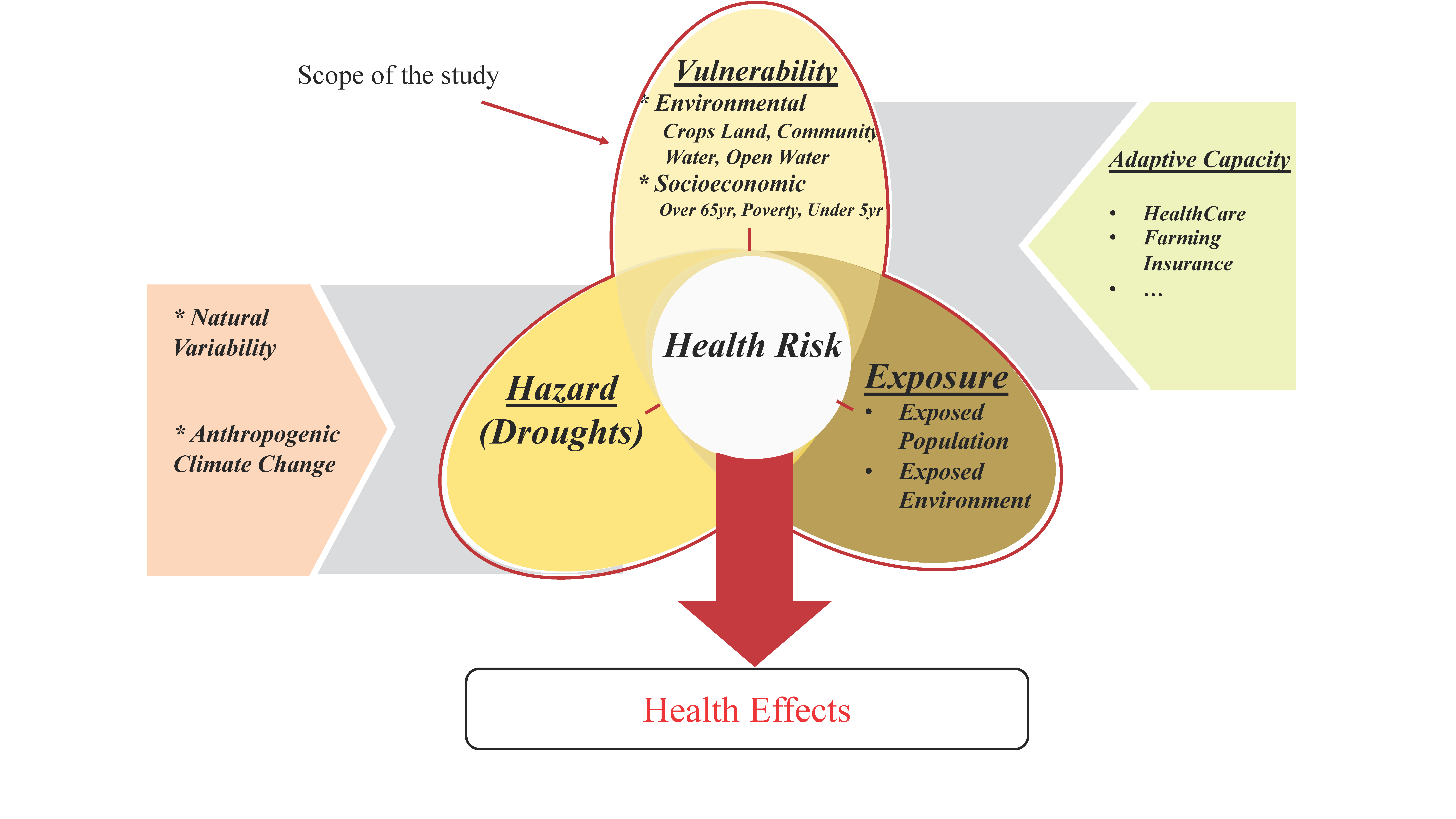
:1. Introduction
2. Materials and Methods
2.1. Data
2.1.1. Vulnerability Variables
2.1.2. Hazard Parameters
2.2. Methods
2.2.1. State-Level Changes in Vulnerability Measures
2.2.2. Local Moran’s I Statistics
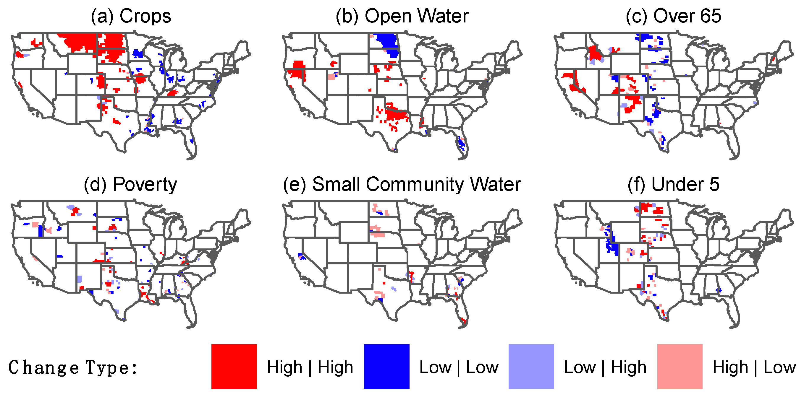
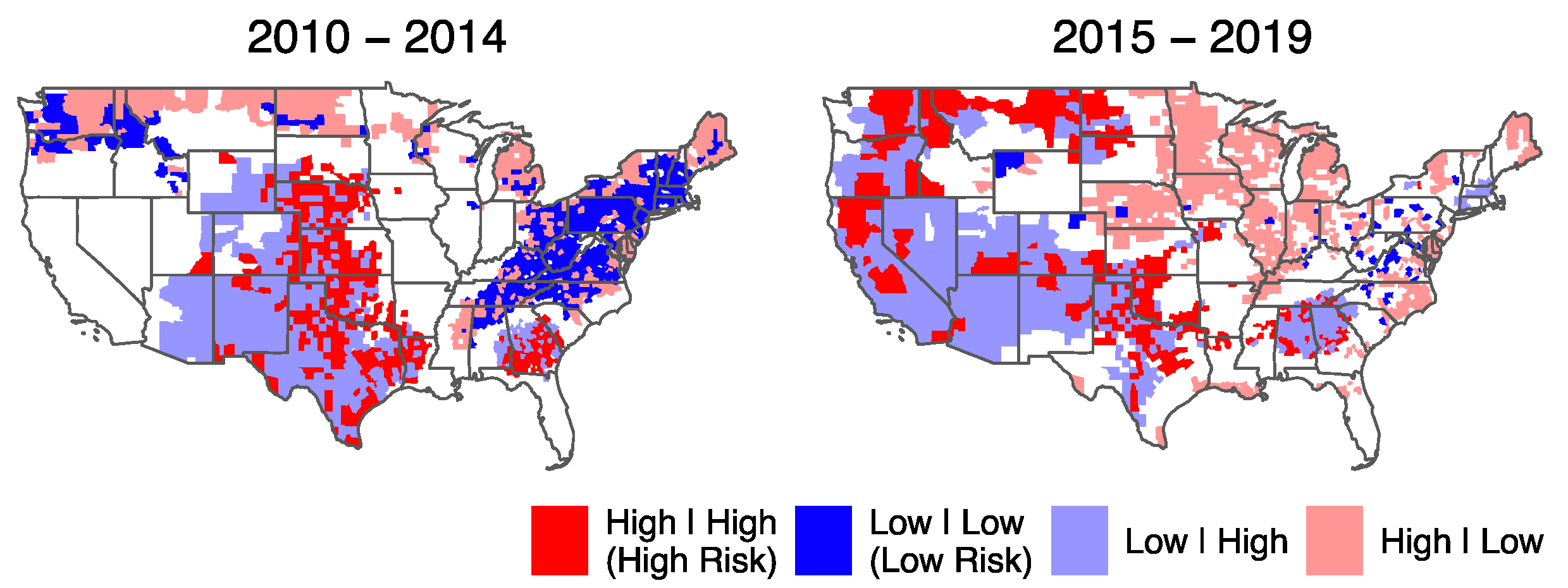
3. Results
3.1. Changes in Hazard
3.2. Vulnerability Variables
3.3. Health Risks
4. Discussion
5. Conclusions
Supplementary Materials
Author Contributions
Funding
Data Availability Statement
Conflicts of Interest
References
- WHO Drought. Available online: https://www.who.int/health-topics/drought#tab=tab_1 (accessed on 5 December 2021).
- Andreadis, K.M.; Lettenmaier, D.P. Trends in 20th century drought over the continental United States. Geophys. Res. Lett. 2006, 33, L10403. [Google Scholar] [CrossRef] [Green Version]
- Kalis, M.A. When every drop counts—Drought guidance for public health professionals. J. Environ. Health 2011, 74, 30–31. [Google Scholar] [PubMed]
- Ficklin, D.L.; Maxwell, J.T.; Letsinger, S.L.; Gholizadeh, H. A climatic deconstruction of recent drought trends in the United States. Environ. Res. Lett. 2015, 10, 044009. [Google Scholar] [CrossRef]
- Peterson, T.C.; Karl, T.R.; Kossin, J.P.; Kunkel, K.E.; Lawrimore, J.H.; McMahon, J.R.; Vose, R.S.; Yin, X. Changes in weather and climate extremes: State of knowledge relevant to air and water quality in the United States. J. Air Waste Manag. Assoc. 2014, 64, 184–197. [Google Scholar] [CrossRef] [Green Version]
- The High Cost of Drought|Drought.gov. Available online: https://www.drought.gov/news/high-cost-drought (accessed on 5 December 2021).
- Salvador, C.; Nieto, R.; Linares, C.; Díaz, J.; Gimeno, L. Quantification of the effects of droughts on daily mortality in spain at different timescales at regional and national levels: A meta-analysis. Int. J. Environ. Res. Public Health 2020, 17, 6114. [Google Scholar] [CrossRef]
- Sugg, M.; Runkle, J.; Leeper, R.; Bagli, H.; Golden, A.; Handwerger, L.H.; Magee, T.; Moreno, C.; Reed-Kelly, R.; Taylor, M.; et al. A scoping review of drought impacts on health and society in North America. Clim. Chang. 2020, 162, 1177–1195. [Google Scholar] [CrossRef]
- Vins, H.; Bell, J.; Saha, S.; Hess, J.J. The mental health outcomes of drought: A systematic review and causal process diagram. Int. J. Environ. Res. Public Health 2015, 12, 13251–13275. [Google Scholar] [CrossRef] [Green Version]
- Bell, J.E.; Herring, S.C.; Jantarasami, L.; Adrianopoli, C.; Benedict, K.; Conlon, K.; Escobar, V.; Hess, J.; Luvall, J.; Garcia-Pando, C.P.; et al. Ch. 4: Impacts of Extreme Events on Human Health. The Impacts of Climate Change on Human Health. In the United States: A Scientific Assessment; US Global Change Research Program: Washington, DC, USA, 2016. [Google Scholar] [CrossRef]
- Berman, J.D.; Ramirez, M.R.; Bell, J.E.; Bilotta, R.; Gerr, F.; Fethke, N.B. The association between drought conditions and increased occupational psychosocial stress among U.S. farmers: An occupational cohort study. Sci. Total Environ. 2021, 798, 149245. [Google Scholar] [CrossRef]
- Bell, J.E.; Brown, C.L.; Conlon, K.; Herring, S.; Kunkel, K.E.; Lawrimore, J.; Luber, G.; Schreck, C.; Smith, A.; Uejio, C. Changes in extreme events and the potential impacts on human health. J. Air Waste Manag. Assoc. 2018, 68, 265–287. [Google Scholar] [CrossRef] [Green Version]
- Ebi, K.L.; Vanos, J.; Baldwin, J.W.; Bell, J.E.; Hondula, D.M.; Errett, N.A.; Hayes, K.; Reid, C.E.; Saha, S.; Spector, J.; et al. Extreme Weather and Climate Change: Population Health and Health System Implications. Annu. Rev. Public Health 2020, 42, 293–315. [Google Scholar] [CrossRef]
- Field, C.; Barros, V.; Stocker, T.; Dahe, Q. Managing the Risks of Extreme Events and Disasters to Advance Climate Change Adaptation: Special Report of the Intergovernmental Panel on Climate Change; Cambridge University Press: Cambridge, UK, 2012. [Google Scholar]
- Birkmann, J.; Mechler, R. Advancing climate adaptation and risk management. New insights, concepts and approaches: What have we learned from the SREX and the AR5 processes? Clim. Chang. 2015, 133, 1–6. [Google Scholar] [CrossRef] [Green Version]
- Ebi, K.L.; Bowen, K. Extreme events as sources of health vulnerability: Drought as an example. Weather Clim. Extrem. 2016, 11, 95–102. [Google Scholar] [CrossRef] [Green Version]
- Sena, A.; Ebi, K.L.; Freitas, C.; Corvalan, C.; Barcellos, C. Indicators to measure risk of disaster associated with drought: Implications for the health sector. PLoS ONE 2017, 12, e0181394. [Google Scholar] [CrossRef] [PubMed]
- UNISDR. Global Assessment Report on Disaster Risk Reduction; UNISDR: Geneva, Switzerland, 2011. [Google Scholar]
- Malik, S.M.; Awan, H.; Khan, N. Mapping vulnerability to climate change and its repercussions on human health in Pakistan. Global. Health 2012, 8, 31. [Google Scholar] [CrossRef] [Green Version]
- McDonald, A. Dried Up: Poverty in America’s Drought Lands. Available online: https://www.deseret.com/2014/6/15/20543158/dried-up-poverty-in-america-s-drought-lands (accessed on 5 December 2021).
- Sena, A.; Barcellos, C.; Freitas, C.; Corvalan, C. Managing the health impacts of drought in Brazil. Int. J. Environ. Res. Public Health 2014, 11, 10737–10751. [Google Scholar] [CrossRef] [PubMed] [Green Version]
- Shriber, J.; Conlon, K.C.; Benedict, K.; McCotter, O.Z.; Bell, J.E. Assessment of vulnerability to coccidioidomycosis in Arizona and California. Int. J. Environ. Res. Public Health 2017, 14, 680. [Google Scholar] [CrossRef] [Green Version]
- Stanke, C.; Kerac, M.; Prudhomme, C.; Medlock, J.; Murray, V. Health Effects of Drought: A Systematic Review of the Evidence. PLoS Curr. 2013, 5. [Google Scholar] [CrossRef] [Green Version]
- Yusa, A.; Berry, P.; Cheng, J.J.; Ogden, N.; Bonsal, B.; Stewart, R.; Waldick, R. Climate change, drought and human health in Canada. Int. J. Environ. Res. Public Health 2015, 12, 8359–8412. [Google Scholar] [CrossRef]
- Gamble, J.L.; Hurley, B.J.; Schultz, P.A.; Jaglom, W.S.; Krishnan, N.; Harris, M. Climate change and older Americans: State of the science. Environ. Health Perspect. 2013, 121, 15–22. [Google Scholar] [CrossRef] [Green Version]
- Hagenlocher, M.; Meza, I.; Anderson, C.C.; Min, A.; Renaud, F.G.; Walz, Y.; Siebert, S.; Sebesvari, Z. Drought vulnerability and risk assessments: State of the art, persistent gaps, and research agenda. Environ. Res. Lett. 2019, 14, 083002. [Google Scholar] [CrossRef]
- Meza, I.; Hegenlocher, M.; Naumann, G.; Vogt, J.V.; Frischen, J. Drought Vulnerability Indicators for Global-Scale Drought Risk Assessments—Global Expert Survey Results Report; Publications Office of the European Union: Luxembourg, 2019; pp. 1–62. [CrossRef]
- Sena, A.; Freitas, C.; Souza, P.F.; Carneiro, F.; Alpino, T.; Pedroso, M.; Corvalan, C.; Barcellos, C. Drought in the Semiarid Region of Brazil: Exposure, Vulnerabilities and Health Impacts from the Perspectives of Local Actors. PLoS Curr. 2018, 10. [Google Scholar] [CrossRef] [PubMed]
- Erian, W.; Pulwarty, R.; Vogt, J.; AbuZeid, K.; Bert, F. GAR Special Report on Drought 2021; United Nations Office for Disaster Risk Reduction (UNDRR): Geneva, Switzerland, 2021. [Google Scholar]
- US Census Bureau. American Community Survey (ACS) 5-Year Estimates; Prepared by Social Explorer; US Census Bureau: Suitland-Silver Hill, MD, USA, 2017.
- Anselin, L. Local Indicators of Spatial Association—LISA. Geogr. Anal. 1995, 27, 93–115. [Google Scholar] [CrossRef]
- Svoboda, M.D.; Fuchs, B.A. Handbook of Drought Indicators and Indices. Drought Water Cris. 2019, 155–208. [Google Scholar] [CrossRef] [Green Version]
- Svoboda, M.; LeComte, D.; Hayes, M.; Heim, R.; Gleason, K.; Angel, J.; Rippey, B.; Tinker, R.; Palecki, M.; Stooksbury, D.; et al. The drought monitor. Bull. Am. Meteorol. Soc. 2002, 83, 1181–1190. [Google Scholar] [CrossRef] [Green Version]
- R Core Development Team. A Language and Environment for Statistical Computing; R Foundation for Statistical Computing: Vienna, Austria, 2020. [Google Scholar]
- Walker, K.; Herman, M. Tidycensus: Load US Census Boundary and Attribute Data as “tidyverse” and ‘sf’-Ready Data Frames; R Package Version 0.11.4; R Foundation for Statistical Computing: Vienna, Austria, 2021. [Google Scholar]
- EPA SDWIS. U.S. Environmental Protection Agency Safe DrinkingWater Information System. Available online: https://ofmpub.epa.gov/apex/sfdw/f?p=108:1::::1 (accessed on 1 December 2021).
- Maskrey, A.; Peduzzi, P.; Chatenoux, B.; Herold, C.; Dao, Q.H.; Giuliani, G. Revealing Risk, Redefining Development, Global Assessment Report on Disaster Risk Reduction; United Nations Strategy for Disaster Reduction: Geneva, Switzerland, 2011; pp. 17–51. [Google Scholar]
- Yang, L.; Jin, S.; Danielson, P.; Homer, C.; Gass, L.; Bender, S.M.; Case, A.; Costello, C.; Dewitz, J.; Fry, J.; et al. A new generation of the United States National Land Cover Database: Requirements, research priorities, design, and implementation strategies. ISPRS J. Photogramm. Remote Sens. 2018, 146, 108–123. [Google Scholar] [CrossRef]
- Corbin, G.T. Learning ArcGIS Pro; Packt Publishing Ltd.: Birmingham, UK, 2015. [Google Scholar]
- Twagirayezu, G.; Nizeyimana, J.C. Generation of Rainfall Intensity Duration Frequency (IDF) Curves for the Solution of Hydraulic Design Problems; LAP LAMBERT Academic Publishing: Saarbrücken, Germany, 2021. [Google Scholar]
- Augustin, T.; Walter, G.; Coolen, F.P.A. Statistical inference. In introduction to Imprecise Probabilities; Wiley: Hoboken, NJ, USA, 2014; pp. 135–189. [Google Scholar] [CrossRef]
- Brown, G.W.; Mood, A.M. On Median Tests for Linear Hypotheses. In Proceedings of the Second Berkeley Symposium on Mathematical Statistics and Probability; University of California Press: Berkeley, CA, USA, 1951; pp. 159–166. [Google Scholar]
- Hothorn, T.; Van De Wiel, M.A.; Hornik, K.; Zeileis, A. Implementing a class of permutation tests: The coin package. J. Stat. Softw. 2008, 28, 1–23. [Google Scholar] [CrossRef]
- Getis, A.; Aldstadt, J. Constructing the spatial weights matrix using a local statistic. Geogr. Anal. 2004, 36, 90–104. [Google Scholar] [CrossRef]
- Anselin, L.; Syabri, I.; Kho, Y. GeoDa: An introduction to spatial data analysis. Geogr. Anal. 2006, 38, 5–22. [Google Scholar] [CrossRef]
- Caldas de Castro, M.; Singer, B.H. Controlling the False Discovery Rate: A New Application to Account for Multiple and Dependent Tests in Local Statistics of Spatial Association. Geogr. Anal. 2006, 38, 180–208. [Google Scholar] [CrossRef]
- Flanagan, B.E.; Hallisey, E.J.; Adams, E.; Lavery, A. Measuring Community Vulnerability to Natural and AnthropogenicHazards: The Centers for Disease Control and Prevention’s SocialVulnerability Index. J. Environ. Health 2018, 80, 34. [Google Scholar]
- Karl, T.R.; Koss, W.J. Regional and National Monthly, Seasonal, and Annual Temperature Weighted by Area, 1895–1983; Historical Climatology Series 4-3; National Climatic Data Center: Asheville, NC, USA, 1984; p. 38.
- Strzepek, K.; Yohe, G.; Neumann, J.; Boehlert, B. Characterizing changes in drought risk for the United States from climate change. Environ. Res. Lett. 2010, 5, 044012. [Google Scholar] [CrossRef]
- Spinoni, J.; Barbosa, P.; Bucchignani, E.; Cassano, J.; Cavazos, T.; Christensen, J.H.; Christensen, O.B.; Coppola, E.; Evans, J.; Geyer, B.; et al. Future Global Meteorological Drought Hot Spots: A Study Based on CORDEX Data. J. Clim. 2020, 33, 3635–3661. [Google Scholar] [CrossRef]
- Berman, J.D.; Ebisu, K.; Peng, R.D.; Dominici, F.; Bell, M.L. Drought and the risk of hospital admissions and mortality in older adults in western USA from 2000 to 2013: A retrospective study. Lancet Planet. Health 2017, 1, e17–e25. [Google Scholar] [CrossRef]
- Dilley, M.; Chen, R.S.; Deichmann, U.; Lerner-Lam, A.L.; Arnold, M. Natural Disaster Hotspots: A Global Risk Analysis. In Natural Disaster Hotspots; World Bank: Washington, DC, USA, 2005. [Google Scholar] [CrossRef]
- Mohammed, R.; Scholz, M. The reconnaissance drought index: A method for detecting regional arid climatic variability and potential drought risk. J. Arid Environ. 2017, 144, 181–191. [Google Scholar] [CrossRef]
- Chou, J.; Xian, T.; Zhao, R.; Xu, Y.; Yang, F.; Sun, M. Drought Risk Assessment and Estimation in Vulnerable Eco-Regions of China: Under the Background of Climate Change. Sustainability 2019, 11, 4463. [Google Scholar] [CrossRef] [Green Version]
- Salvador, C.; Nieto, R.; Linares, C.; Díaz, J.; Gimeno, L. Effects of droughts on health: Diagnosis, repercussion, and adaptation in vulnerable regions under climate change. Challenges for future research. Sci. Total Environ. 2020, 703, 134912. [Google Scholar] [CrossRef] [PubMed]
- Lynch, K.M.; Lyles, R.H.; Waller, L.A.; Abadi, A.M.; Bell, J.E.; Gribble, M.O. Drought severity and all-cause mortality rates among adults in the United States: 1968–2014. Environ. Health 2020, 19, 52. [Google Scholar] [CrossRef]
- Belesova, K.; Agabiirwe, C.N.; Zou, M.; Phalkey, R.; Wilkinson, P. Drought exposure as a risk factor for child undernutrition in low- and middle-income countries: A systematic review and assessment of empirical evidence. Environ. Int. 2019, 131, 104973. [Google Scholar] [CrossRef]
- Balbus, J. Understanding drought’s impacts on human health. Lancet Planet. Health 2017, 1, e12. [Google Scholar] [CrossRef]
- Mihunov, V.V.; Lam, N.S.N.; Zou, L.; Rohli, R.V.; Bushra, N.; Reams, M.A.; Argote, J.E. Community Resilience to Drought Hazard in the South-Central United States. Ann. Am. Assoc. Geogr. 2017, 108, 739–755. [Google Scholar] [CrossRef]
- Assunção, R.M.; Reis, E.A. A new proposal to adjust Moran’s I for population density. Stat. Med. 1999, 18, 2147–2162. [Google Scholar] [CrossRef]
- Tsai, P.J. Application of Moran’s test with an empirical Bayesian rate to leading health care problems in Taiwan in a 7-year period (2002–2008). Glob. J. Health Sci. 2012, 4, 63–77. [Google Scholar] [CrossRef] [PubMed]
- American Community Survey 5-Year Data (2009–2020). Available online: https://www.census.gov/data/developers/data-sets/acs-5year.html (accessed on 5 December 2021).
- Safe Drinking Water Information System (SDWIS) Federal Reporting Services. Available online: https://www.epa.gov/ground-water-and-drinking-water/safe-drinking-water-information-system-sdwis-federal-reporting (accessed on 20 November 2021).
- Data. Multi-Resolution Land Characteristic Consortium (MRLC). Available online: https://www.mrlc.gov/data (accessed on 20 November 2021).
- Comprehensive Statistics. US Drought Monitor. Available online: https://droughtmonitor.unl.edu/DmData/DataDownload/ComprehensiveStatistics.aspx (accessed on 20 November 2021).
- Jalalzadeh Fard, B. Evaluating Changes in Health Risk from Drought Over the Contiguous United States. Mendeley Data 2022. [Google Scholar] [CrossRef]


| State | Over 65 | Poverty | Under 5 |
|---|---|---|---|
| Alabama | 2.56 | −1.94 | −0.14 |
| Arkansas | 1.84 | −1.49 | - |
| Colorado | 2.58 | - | - |
| Florida | 2.47 | −2.07 | −0.29 |
| Georgia | 2.05 | - | −0.38 |
| Illinois | 1.62 | - | - |
| Indiana | 2.03 | - | - |
| Iowa | 1.42 | - | - |
| Kentucky | 2.08 | - | - |
| Louisiana | 2.01 | - | - |
| Maryland | 1.96 | - | - |
| Michigan | 2.47 | −1.39 | - |
| Minnesota | - | −1.25 | - |
| Mississippi | 1.96 | - | −0.49 |
| Missouri | 1.71 | −1.80 | - |
| Nebraska | - | −1.00 | - |
| New Jersey | 3.13 | - | - |
| New York | 2.29 | - | - |
| North Carolina | 2.81 | −2.36 | −0.40 |
| Ohio | 1.87 | −1.36 | - |
| Oklahoma | 1.30 | - | - |
| Oregon | - | −3.20 | - |
| Pennsylvania | 1.92 | - | - |
| South Caroli- | 2.63 | - | −0.46 |
| Tennessee | 2.18 | −1.81 | - |
| Texas | 1.41 | −1.32 | - |
| Utah | - | - | −0.84 |
| Virginia | 2.21 | - | - |
| West Virginia | 2.75 | - | - |
| Wisconsin | 2.13 | −1.12 | - |
Publisher’s Note: MDPI stays neutral with regard to jurisdictional claims in published maps and institutional affiliations. |
© 2022 by the authors. Licensee MDPI, Basel, Switzerland. This article is an open access article distributed under the terms and conditions of the Creative Commons Attribution (CC BY) license (https://creativecommons.org/licenses/by/4.0/).
Share and Cite
Jalalzadeh Fard, B.; Puvvula, J.; Bell, J.E. Evaluating Changes in Health Risk from Drought over the Contiguous United States. Int. J. Environ. Res. Public Health 2022, 19, 4628. https://doi.org/10.3390/ijerph19084628
Jalalzadeh Fard B, Puvvula J, Bell JE. Evaluating Changes in Health Risk from Drought over the Contiguous United States. International Journal of Environmental Research and Public Health. 2022; 19(8):4628. https://doi.org/10.3390/ijerph19084628
Chicago/Turabian StyleJalalzadeh Fard, Babak, Jagadeesh Puvvula, and Jesse E. Bell. 2022. "Evaluating Changes in Health Risk from Drought over the Contiguous United States" International Journal of Environmental Research and Public Health 19, no. 8: 4628. https://doi.org/10.3390/ijerph19084628
APA StyleJalalzadeh Fard, B., Puvvula, J., & Bell, J. E. (2022). Evaluating Changes in Health Risk from Drought over the Contiguous United States. International Journal of Environmental Research and Public Health, 19(8), 4628. https://doi.org/10.3390/ijerph19084628