
Using a Novel Functional Brain Network Approach to Locate Important Nodes for Working Memory Tasks


Abstract
:1. Introduction
2. Experiment
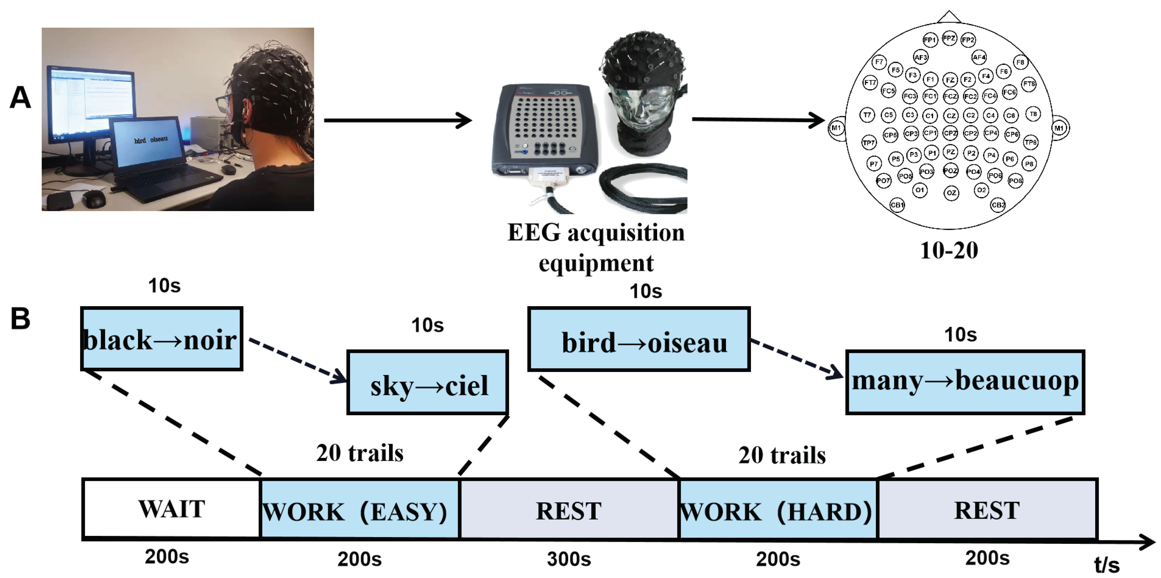
2.1. Experiment Paradigm
2.2. Subject Qualification
2.3. EEG Recording
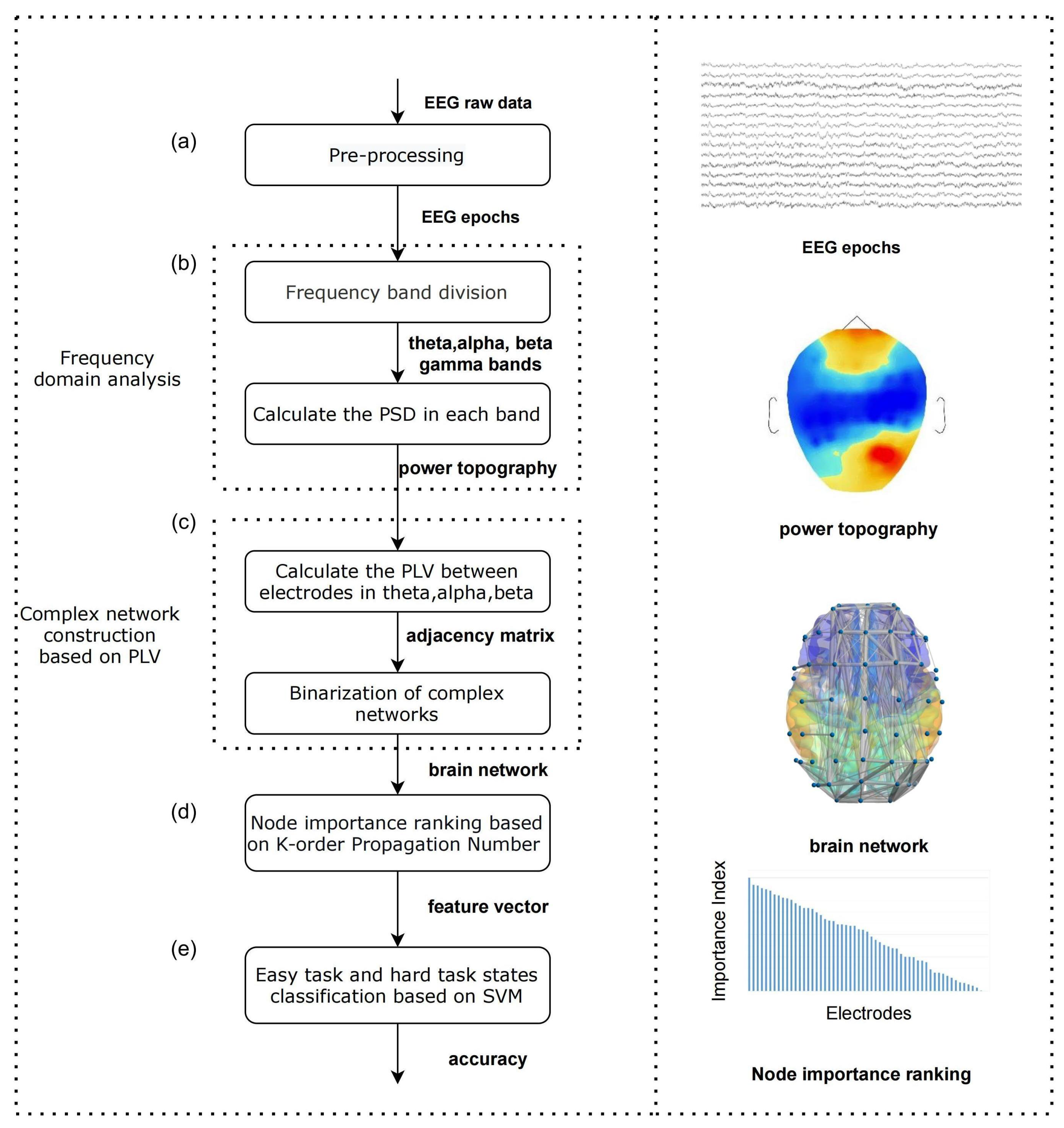
3. Method
3.1. Algorithm Configuration
3.2. EEG Data Pre-Processing
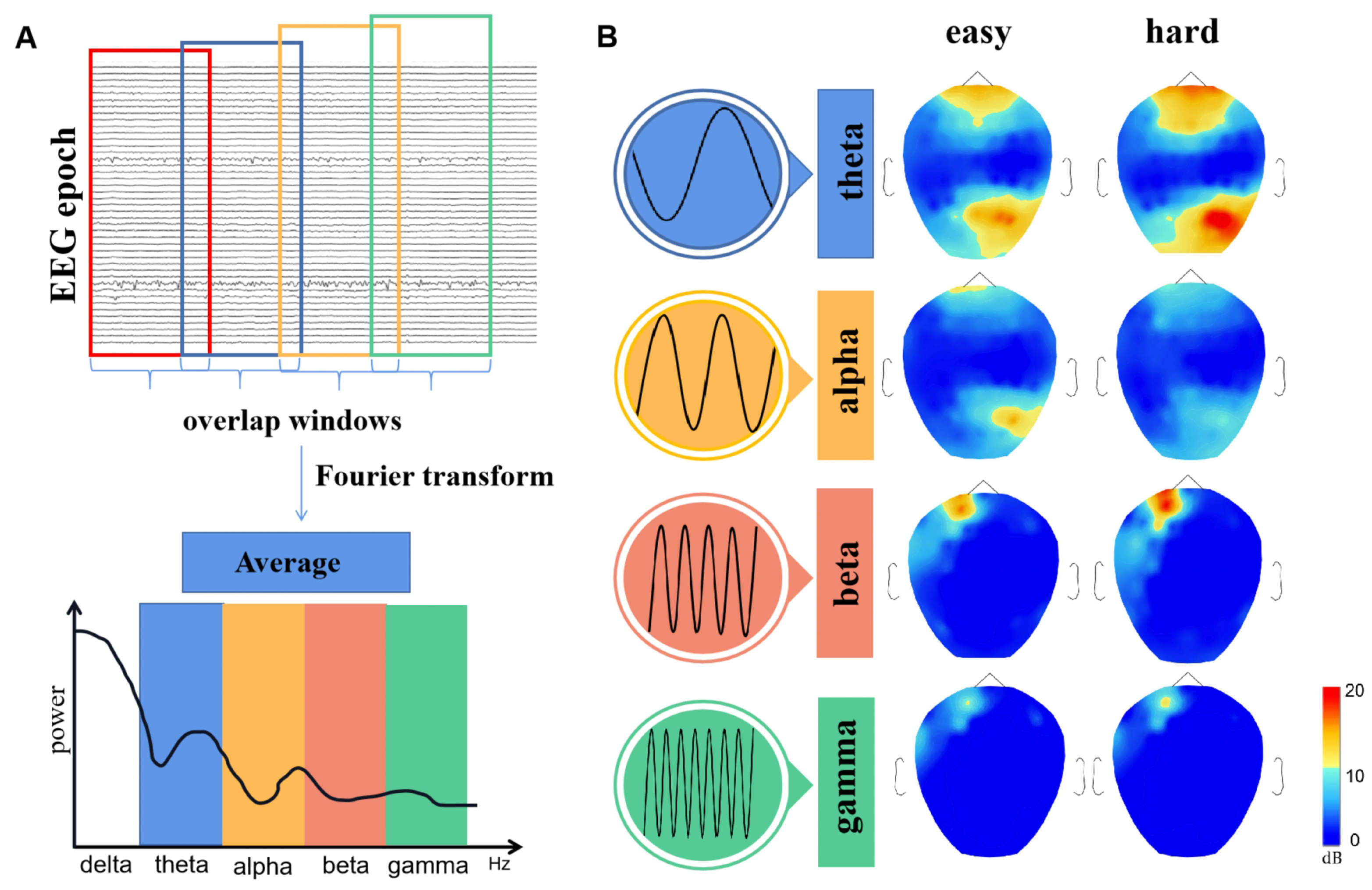
3.3. Frequency Domain Analysis
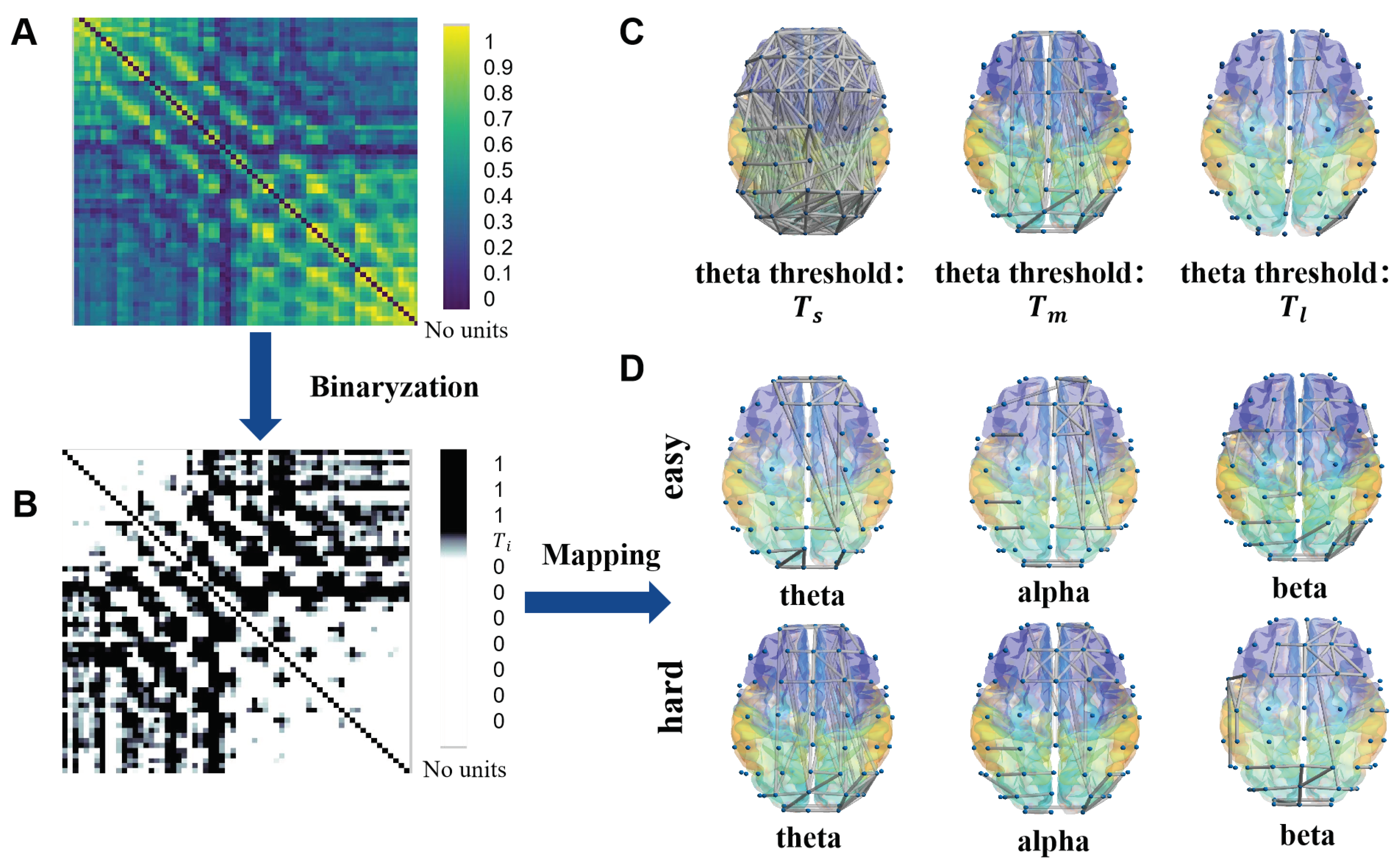
3.4. Complex Network Construction Based on Phase Lock Value
3.5. Node Importance Based on K-Order Propagation Number Algorithm
3.6. Different Memory Load States Classification Based on SVM
4. Result
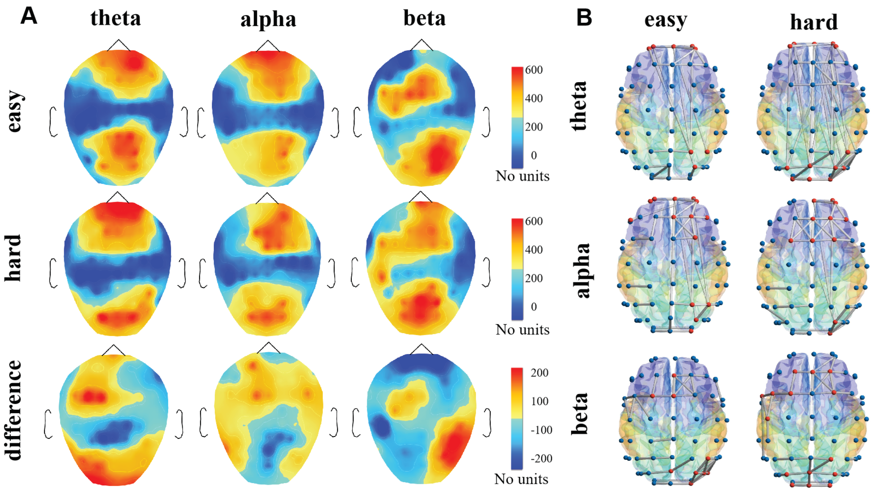
4.1. The Nodes Importance of Brain Network
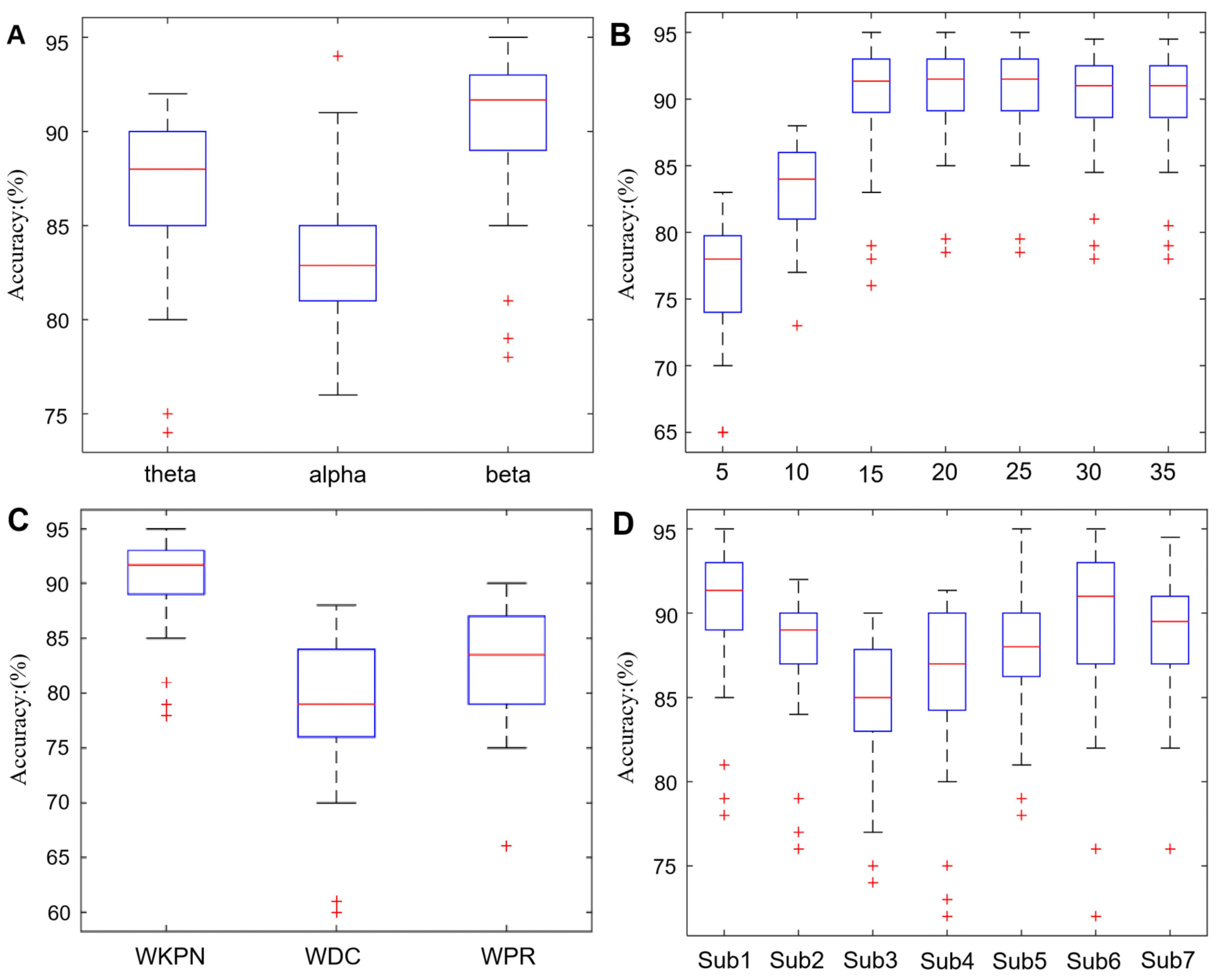
4.2. The Classification Accuracy of SVM
5. Discussion and Conclusions
Author Contributions
Funding
Institutional Review Board Statement
Informed Consent Statement
Data Availability Statement
Conflicts of Interest
References
- Engle, R.W. Working memory and executive attention: A revisit. Perspect. Psychol. Sci. 2018, 13, 190–193. [Google Scholar] [CrossRef] [PubMed]
- Rasmussen, J.; Langerman, H. Alzheimer’s disease—Why we need early diagnosis. Degener. Neurol. Neuromuscul. Dis. 2019, 9, 123–130. [Google Scholar] [CrossRef] [PubMed] [Green Version]
- Aghababaiyan, K.; Shah-Mansouri, V.; Maham, B. Asynchronous neuro-spike array-based communication. In Proceedings of the 2018 IEEE International Black Sea Conference on Communications and Networking (BlackSeaCom), Batumi, Georgia, 4–7 June 2018; pp. 1–5. [Google Scholar]
- Aghababaiyan, K.; Shah-Mansouri, V.; Maham, B. Capacity and error probability analysis of neuro-spike communication exploiting temporal modulation. IEEE Trans. Commun. 2019, 68, 2078–2089. [Google Scholar] [CrossRef]
- Michels, L.; Bucher, K.; Lüchinger, R.; Klaver, P.; Martin, E.; Jeanmonod, D.; Brandeis, D. Simultaneous EEG-fMRI during a working memory task: Modulations in low and high frequency bands. PLoS ONE 2010, 5, e10298. [Google Scholar] [CrossRef] [PubMed]
- Bae, G.Y.; Luck, S.J. Dissociable decoding of spatial attention and working memory from EEG oscillations and sustained potentials. J. Neurosci. 2018, 38, 409–422. [Google Scholar] [CrossRef] [PubMed] [Green Version]
- Zhang, Y.; Wang, C.; Wu, F.; Huang, K.; Yang, L.; Ji, L. Prediction of working memory ability based on EEG by functional data analysis. J. Neurosci. Methods 2020, 333, 108552. [Google Scholar] [CrossRef] [PubMed]
- Günseli, E.; Fahrenfort, J.J.; van Moorselaar, D.; Daoultzis, K.C.; Meeter, M.; Olivers, C.N. EEG dynamics reveal a dissociation between storage and selective attention within working memory. Sci. Rep. 2019, 9, 13499. [Google Scholar] [CrossRef]
- Makino, H.; Komiyama, T. Learning enhances the relative impact of top-down processing in the visual cortex. Nat. Neurosci. 2015, 18, 1116–1122. [Google Scholar] [CrossRef]
- Fries, P. Rhythms for cognition: Communication through coherence. Neuron 2015, 88, 220–235. [Google Scholar] [CrossRef] [Green Version]
- Bressler, S.L.; Richter, C.G. Interareal oscillatory synchronization in top-down neocortical processing. Curr. Opin. Neurobiol. 2015, 31, 62–66. [Google Scholar] [CrossRef]
- Becker, R.; Van De Ville, D.; Kleinschmidt, A. Alpha oscillations reduce temporal long-range dependence in spontaneous human brain activity. J. Neurosci. 2018, 38, 755–764. [Google Scholar] [CrossRef] [PubMed] [Green Version]
- Tomasi, D.; Volkow, N.D. Aging and functional brain networks. Mol. Psychiatry 2012, 17, 549–558. [Google Scholar] [CrossRef] [PubMed]
- Andrews-Hanna, J.R.; Snyder, A.Z.; Vincent, J.L.; Lustig, C.; Head, D.; Raichle, M.E.; Buckner, R.L. Disruption of large-scale brain systems in advanced aging. Neuron 2007, 56, 924–935. [Google Scholar] [CrossRef] [PubMed] [Green Version]
- Gevins, A.; Smith, M.E.; McEvoy, L.; Yu, D. High-resolution EEG mapping of cortical activation related to working memory: Effects of task difficulty, type of processing, and practice. Cereb. Cortex 1997, 7, 374–385. [Google Scholar] [CrossRef] [PubMed] [Green Version]
- Rutishauser, U.; Ross, I.B.; Mamelak, A.N.; Schuman, E.M. Human memory strength is predicted by theta-frequency phase-locking of single neurons. Nature 2010, 464, 903–907. [Google Scholar] [CrossRef] [Green Version]
- Fell, J.; Axmacher, N. The role of phase synchronization in memory processes. Nat. Rev. Neurosci. 2011, 12, 105–118. [Google Scholar] [CrossRef]
- Axmacher, N.; Henseler, M.M.; Jensen, O.; Weinreich, I.; Elger, C.E.; Fell, J. Cross-frequency coupling supports multi-item working memory in the human hippocampus. Proc. Natl. Acad. Sci. USA 2010, 107, 3228–3233. [Google Scholar] [CrossRef] [Green Version]
- Luck, S.J. An Introduction to the Event-Related Potential Technique; MIT Press: Cambridge, MA, USA, 2014. [Google Scholar]
- Baddeley, A.D.; Hitch, G.J.; Allen, R.J. From short-term store to multicomponent working memory: The role of the modal model. Mem. Cogn. 2019, 47, 575–588. [Google Scholar] [CrossRef] [Green Version]
- Stam, C.V.; Van Straaten, E. The organization of physiological brain networks. Clin. Neurophysiol. 2012, 123, 1067–1087. [Google Scholar] [CrossRef]
- Sporns, O. Contributions and challenges for network models in cognitive neuroscience. Nat. Neurosci. 2014, 17, 652–660. [Google Scholar] [CrossRef]
- Bullmore, E.; Sporns, O. The economy of brain network organization. Nat. Rev. Neurosci. 2012, 13, 336–349. [Google Scholar] [CrossRef] [PubMed]
- Fornito, A.; Zalesky, A.; Bullmore, E. Fundamentals of Brain Network Analysis; Academic Press: Cambridge, MA, USA, 2016. [Google Scholar]
- Van Den Heuvel, M.P.; Pol, H.E.H. Exploring the brain network: A review on resting-state fMRI functional connectivity. Eur. Neuropsychopharmacol. 2010, 20, 519–534. [Google Scholar] [CrossRef] [PubMed]
- Hwang, K.; Bertolero, M.A.; Liu, W.B.; D’Esposito, M. The human thalamus is an integrative hub for functional brain networks. J. Neurosci. 2017, 37, 5594–5607. [Google Scholar] [CrossRef] [PubMed] [Green Version]
- Kitzbichler, M.G.; Henson, R.N.; Smith, M.L.; Nathan, P.J.; Bullmore, E.T. Cognitive effort drives workspace configuration of human brain functional networks. J. Neurosci. 2011, 31, 8259–8270. [Google Scholar] [CrossRef] [PubMed] [Green Version]
- Bashivan, P.; Yeasin, M.; Bidelman, G.M. Modulation of brain connectivity by memory load in a working memory network. In Proceedings of the 2014 IEEE Symposium on Computational Intelligence, Cognitive Algorithms, Mind, and Brain (CCMB), Orlando, FL, USA, 9–12 December 2014; pp. 127–133. [Google Scholar]
- Smith, S.M.; Vidaurre, D.; Beckmann, C.F.; Glasser, M.F.; Jenkinson, M.; Miller, K.L.; Nichols, T.E.; Robinson, E.C.; Salimi-Khorshidi, G.; Woolrich, M.W.; et al. Functional connectomics from resting-state fMRI. Trends Cogn. Sci. 2013, 17, 666–682. [Google Scholar] [CrossRef] [PubMed] [Green Version]
- Hurtado, J.M.; Rubchinsky, L.L.; Sigvardt, K.A. Statistical method for detection of phase-locking episodes in neural oscillations. J. Neurophysiol. 2004, 91, 1883–1898. [Google Scholar] [CrossRef] [PubMed]
- Tang, P.; Song, C.; Ding, W.; Ma, J.; Dong, J.; Huang, L. Research on the node importance of a weighted network based on the k-order propagation number algorithm. Entropy 2020, 22, 364. [Google Scholar] [CrossRef] [Green Version]
- Opsahl, T.; Agneessens, F.; Skvoretz, J. Node centrality in weighted networks: Generalizing degree and shortest paths. Soc. Netw. 2010, 32, 245–251. [Google Scholar] [CrossRef]
- Page, L.; Brin, S.; Motwani, R.; Winograd, T. The PageRank Citation Ranking: Bringing Order to the Web; Technical Report; Stanford InfoLab: Stanford, CA, USA, 1999. [Google Scholar]
- Rypma, B.; D’Esposito, M. The roles of prefrontal brain regions in components of working memory: Effects of memory load and individual differences. Proc. Natl. Acad. Sci. USA 1999, 96, 6558–6563. [Google Scholar] [CrossRef] [Green Version]
- Tadel, F.; Baillet, S.; Mosher, J.C.; Pantazis, D.; Leahy, R.M. Brainstorm: A user-friendly application for MEG/EEG analysis. Comput. Intell. Neurosci. 2011, 2011, 879716. [Google Scholar] [CrossRef]
- Delorme, A.; Makeig, S. EEGLAB: An open source toolbox for analysis of single-trial EEG dynamics including independent component analysis. J. Neurosci. Methods 2004, 134, 9–21. [Google Scholar] [CrossRef] [PubMed] [Green Version]
- Cohen, M.X. Analyzing Neural Time Series Data: Theory and Practice; MIT Press: Cambridge, CA, USA, 2014. [Google Scholar]
- Knyazev, G.G. EEG delta oscillations as a correlate of basic homeostatic and motivational processes. Neurosci. Biobehav. Rev. 2012, 36, 677–695. [Google Scholar] [CrossRef] [PubMed]
- Newson, J.J.; Thiagarajan, T.C. EEG frequency bands in psychiatric disorders: A review of resting state studies. Front. Hum. Neurosci. 2019, 12, 521. [Google Scholar] [CrossRef] [PubMed]
- Klimesch, W. Memory processes, brain oscillations and EEG synchronization. Int. J. Psychophysiol. 1996, 24, 61–100. [Google Scholar] [CrossRef]
- Xia, M.; Wang, J.; He, Y. BrainNet Viewer: A network visualization tool for human brain connectomics. PLoS ONE 2013, 8, e68910. [Google Scholar] [CrossRef] [PubMed] [Green Version]
- Sarnthein, J.; Petsche, H.; Rappelsberger, P.; Shaw, G.; Von Stein, A. Synchronization between prefrontal and posterior association cortex during human working memory. Proc. Natl. Acad. Sci. USA 1998, 95, 7092–7096. [Google Scholar] [CrossRef] [PubMed] [Green Version]
- Zhang, Y.; Liao, Y.; Zhang, Y.; Huang, L. Emergency Braking Intention Detect System Based on K-Order Propagation Number Algorithm: A Network Perspective. Brain Sci. 2021, 11, 1424. [Google Scholar] [CrossRef]
- Joachims, T. Making Large-Scale SVM Learning Practical; Technical Report; MIT Press: Cambridge, CA, USA, 1998. [Google Scholar]
- Helfrich, R.F.; Schneider, T.R.; Rach, S.; Trautmann-Lengsfeld, S.A.; Engel, A.K.; Herrmann, C.S. Entrainment of brain oscillations by transcranial alternating current stimulation. Curr. Biol. 2014, 24, 333–339. [Google Scholar] [CrossRef] [Green Version]
- Helfrich, R.F.; Knepper, H.; Nolte, G.; Strüber, D.; Rach, S.; Herrmann, C.S.; Schneider, T.R.; Engel, A.K. Selective modulation of interhemispheric functional connectivity by HD-tACS shapes perception. PLoS Biol. 2014, 12, e1002031. [Google Scholar] [CrossRef] [Green Version]
- Reinhart, R.M.; Nguyen, J.A. Working memory revived in older adults by synchronizing rhythmic brain circuits. Nat. Neurosci. 2019, 22, 820–827. [Google Scholar] [CrossRef] [Green Version]


Publisher’s Note: MDPI stays neutral with regard to jurisdictional claims in published maps and institutional affiliations. |
© 2022 by the authors. Licensee MDPI, Basel, Switzerland. This article is an open access article distributed under the terms and conditions of the Creative Commons Attribution (CC BY) license (https://creativecommons.org/licenses/by/4.0/).
Share and Cite
Ding, W.; Zhang, Y.; Huang, L. Using a Novel Functional Brain Network Approach to Locate Important Nodes for Working Memory Tasks. Int. J. Environ. Res. Public Health 2022, 19, 3564. https://doi.org/10.3390/ijerph19063564
Ding W, Zhang Y, Huang L. Using a Novel Functional Brain Network Approach to Locate Important Nodes for Working Memory Tasks. International Journal of Environmental Research and Public Health. 2022; 19(6):3564. https://doi.org/10.3390/ijerph19063564
Chicago/Turabian StyleDing, Weiwei, Yuhong Zhang, and Liya Huang. 2022. "Using a Novel Functional Brain Network Approach to Locate Important Nodes for Working Memory Tasks" International Journal of Environmental Research and Public Health 19, no. 6: 3564. https://doi.org/10.3390/ijerph19063564
APA StyleDing, W., Zhang, Y., & Huang, L. (2022). Using a Novel Functional Brain Network Approach to Locate Important Nodes for Working Memory Tasks. International Journal of Environmental Research and Public Health, 19(6), 3564. https://doi.org/10.3390/ijerph19063564