
Predicting and Analyzing Road Traffic Injury Severity Using Boosting-Based Ensemble Learning Models with SHAPley Additive exPlanations


Abstract
:1. Introduction
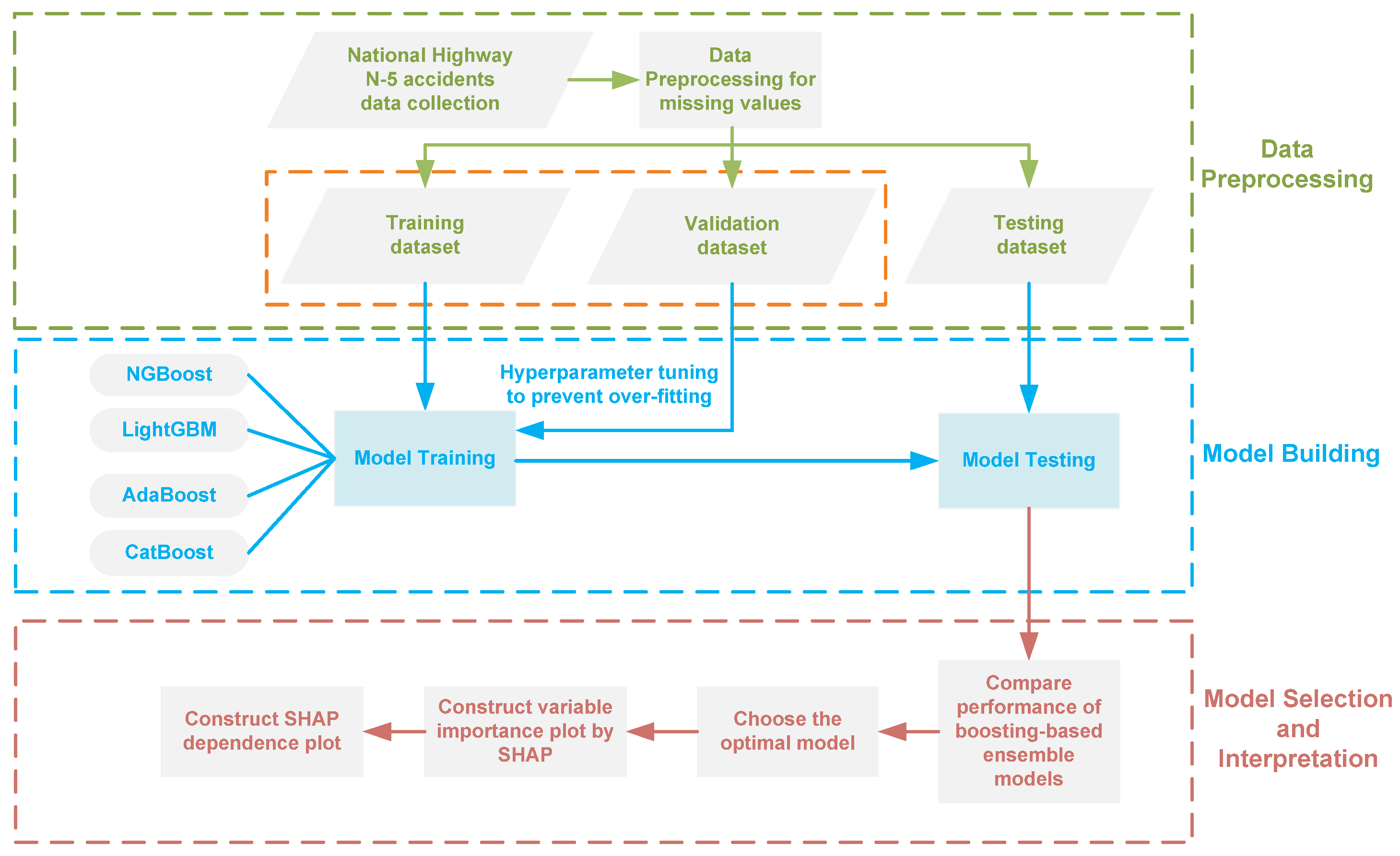
2. Methodology
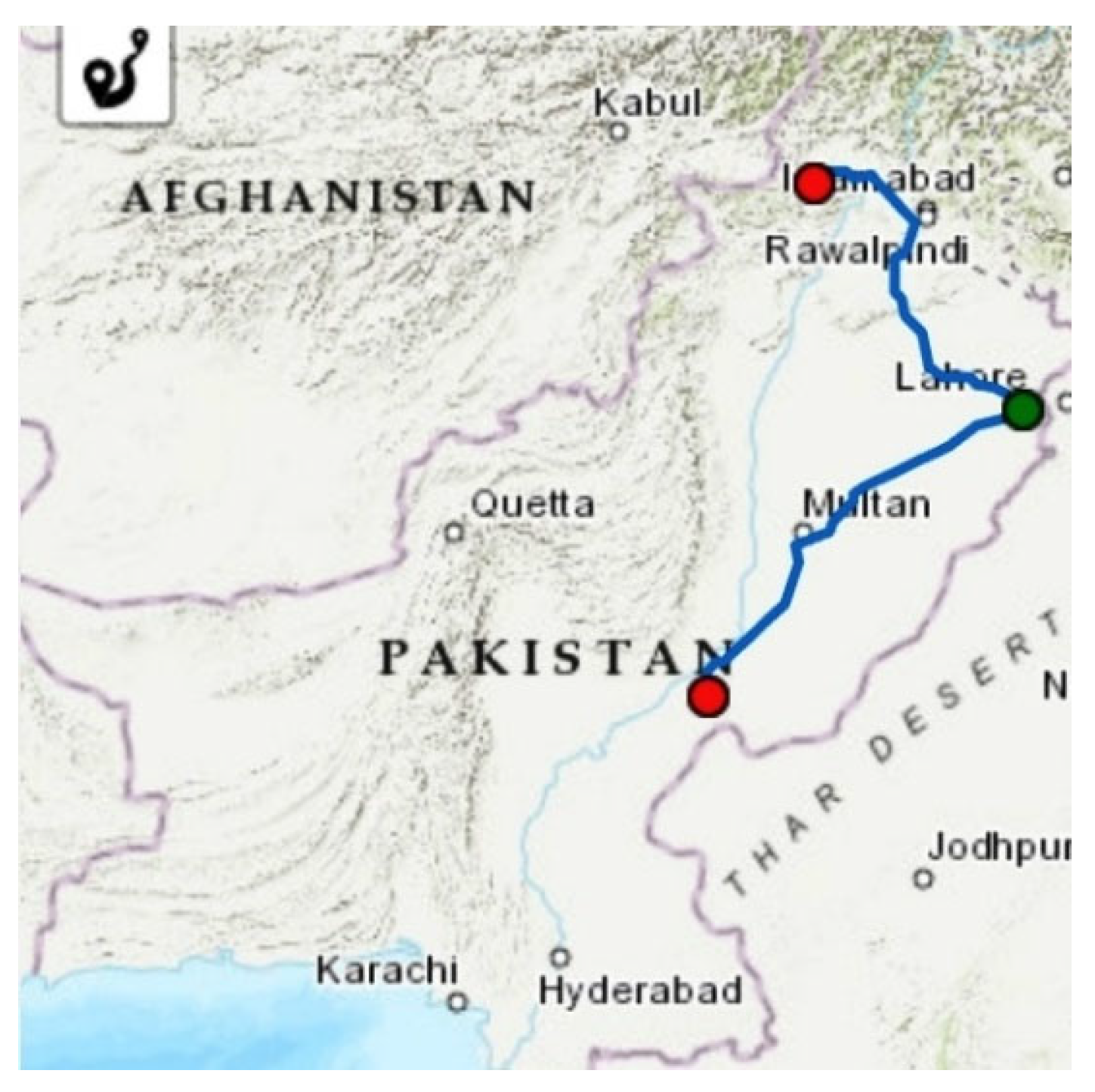
2.1. Study Route
2.2. Data Description
2.3. Boosting-Based Ensemble Learning Classification Models for Injury Severity
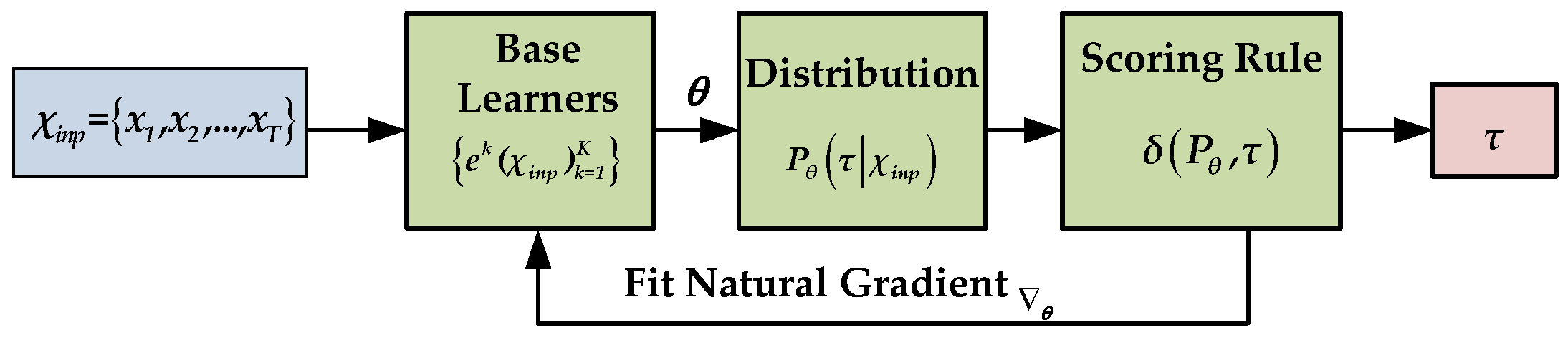
2.3.1. Natural Gradient Boosting (NGBoost)
2.3.2. Categorical Boosting (CatBoost)
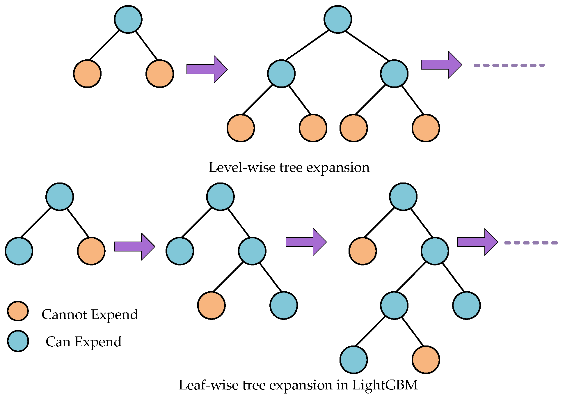
2.3.3. Light Gradient Boosting Machine (LightGBM)
2.3.4. Adaptive Boosting (AdaBoost)
- Initially, all the data points are assigned some equal weights i.e.,:
- For iterations , Train weak learner using distribution , Get weak hypothesis and Select with low weighted error i.e., . Choose .
- Update, to obtain as Equation (9):where is a normalization factor (chosen such that will be a distribution).
- After learning process and weight optimization, the final strong classifier is obtained (Equation (10)), which is based on a linear combination of all the weak classifiers:
2.4. Hyperparameter Tuning
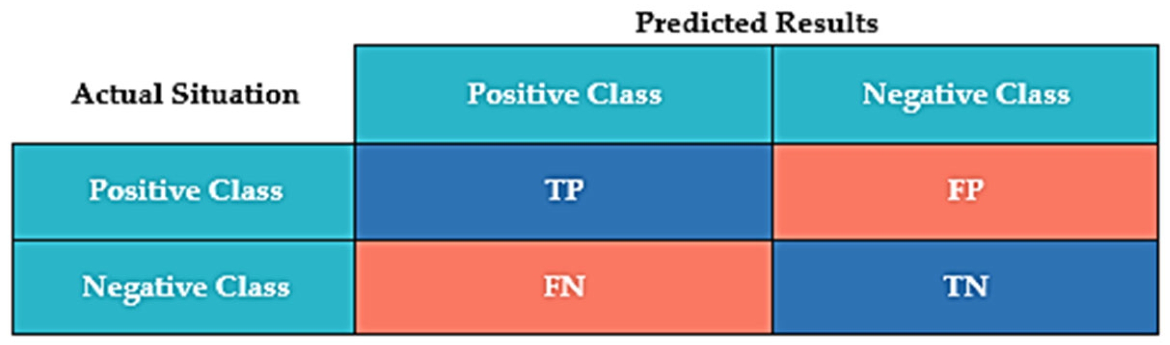
2.5. Model Evaluation
2.6. Model Interpretation
- Local accuracy is defined as the sum of all variable contributions equal to the model’s output. This property fulfills a fundamental requirement of the additive explanatory framework, given by Equation (17):where represents the SHAP value corresponding to variable , is an indicator function that takes the value 1 when the variable appears, and 0 otherwise.
- Absence i.e., the contribution of missing variable is zero. Not that a characteristic value in the structured data is empty, but that a characteristic is not observed in the sample, that is,
- Consistency, i.e., if the model structure alters but the degree to which a particular variable influences the output increases or remains constant, the contribution of that variable to the whole will also enhance or remain constant.
3. Results
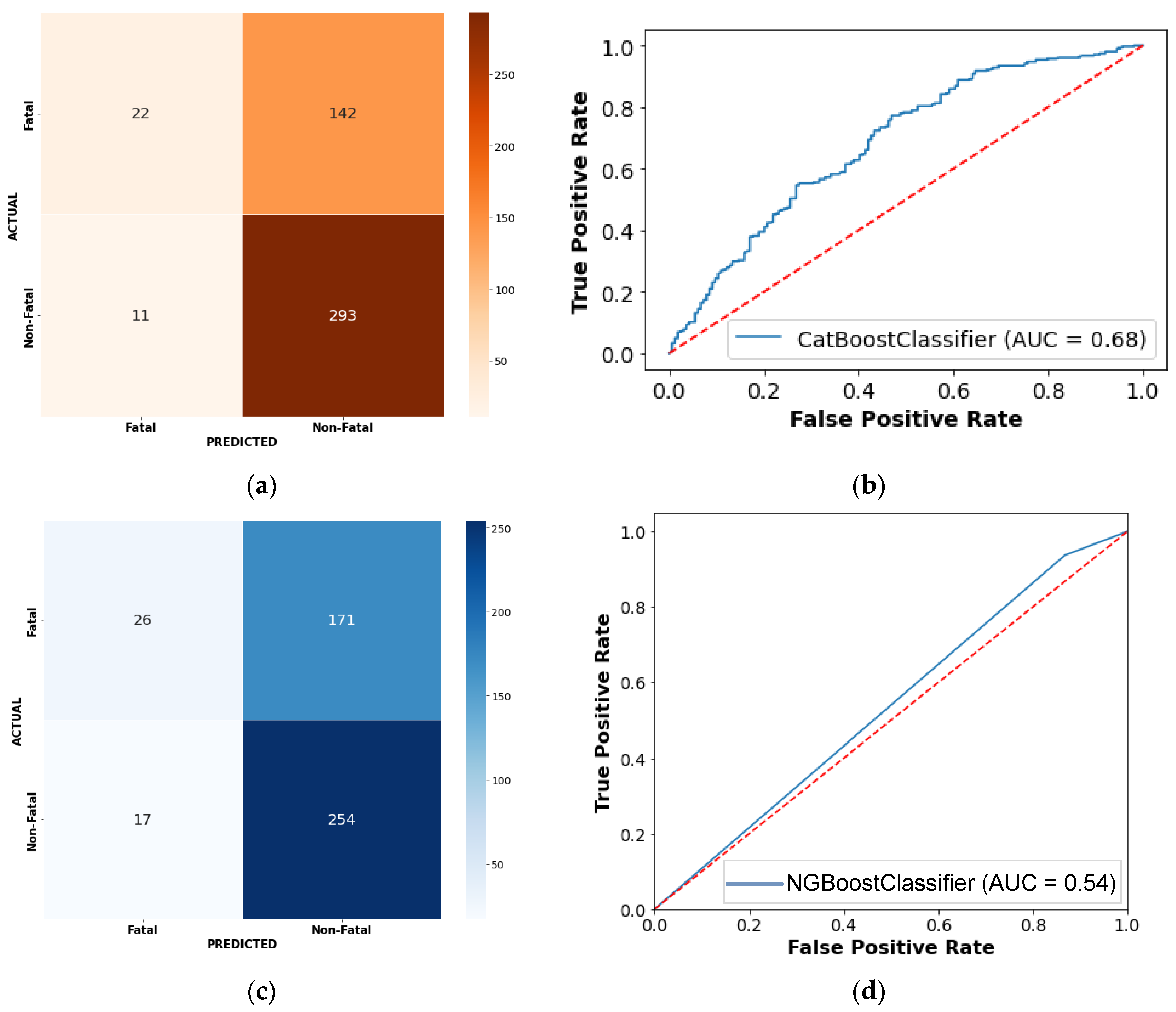
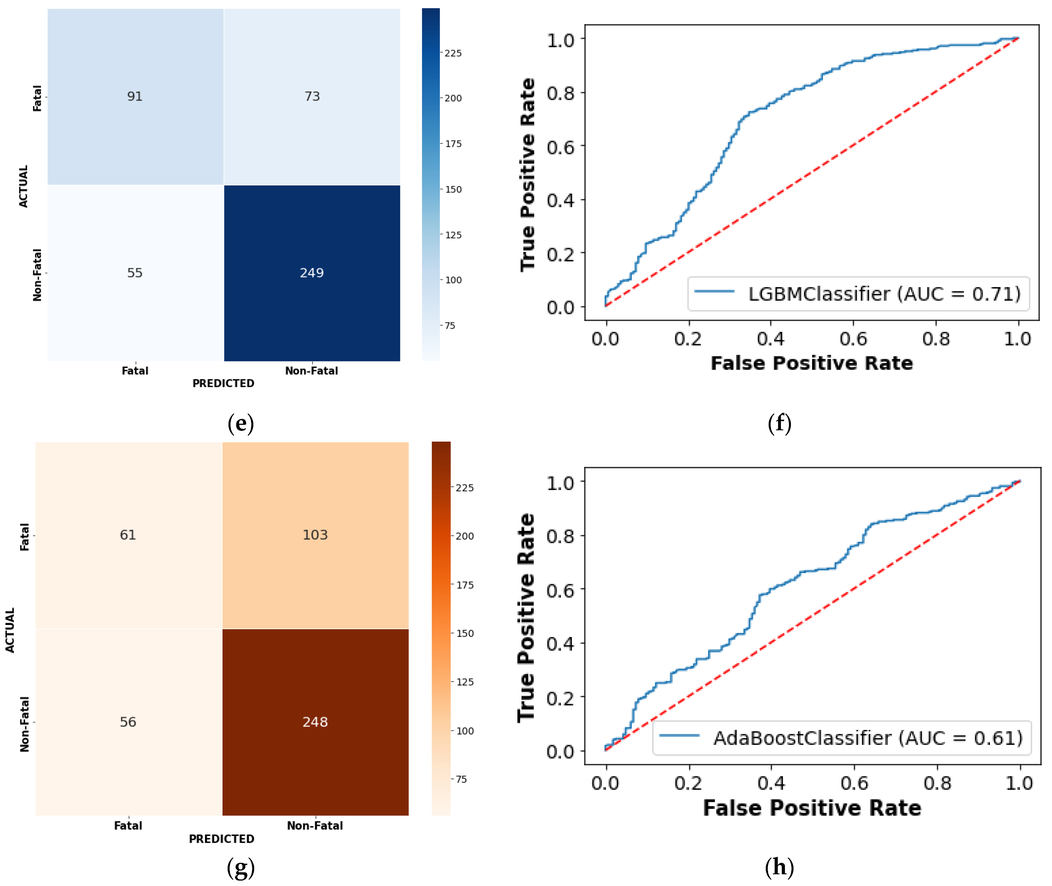
3.1. Performance Assessment
3.2. The Framework of Model Interpretation for Variable
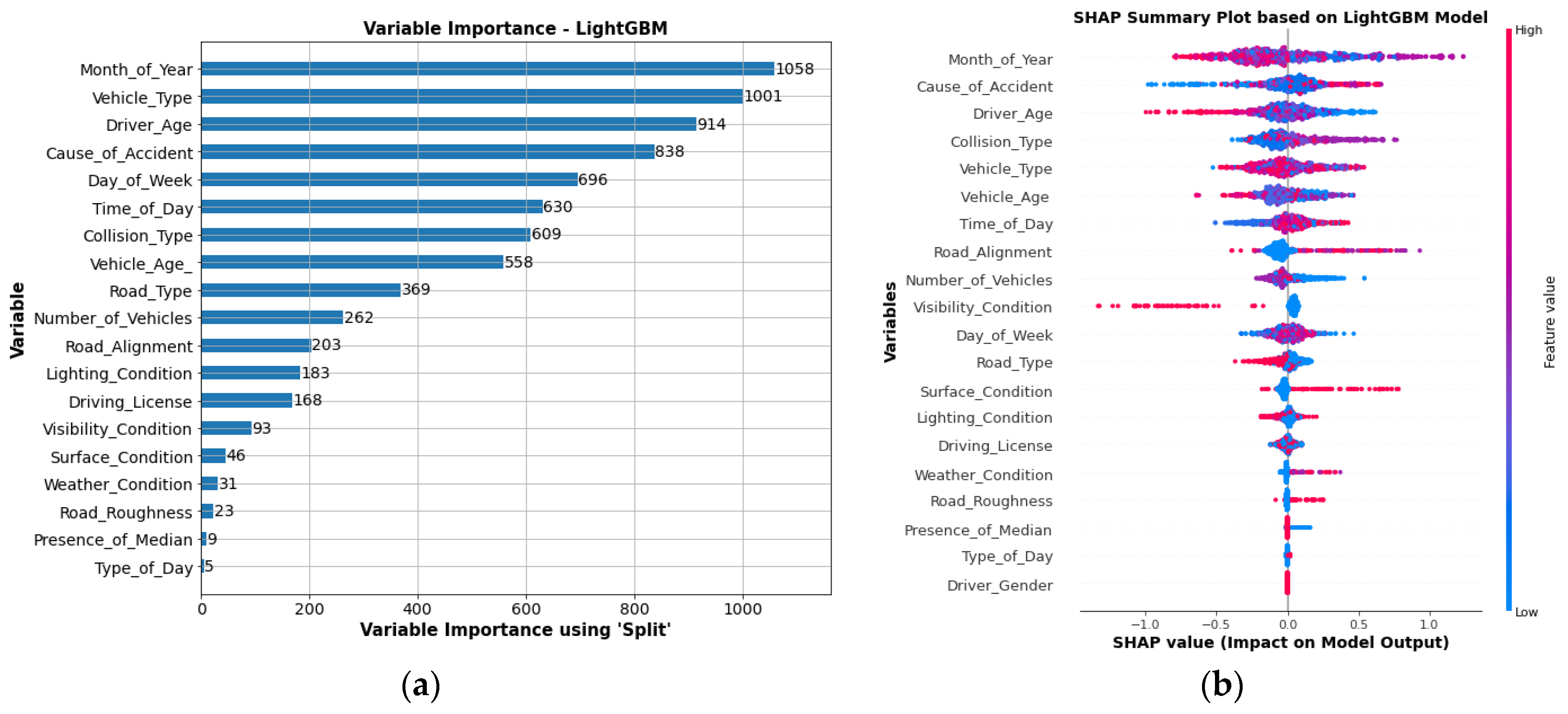
3.2.1. Global Variable Interpretation
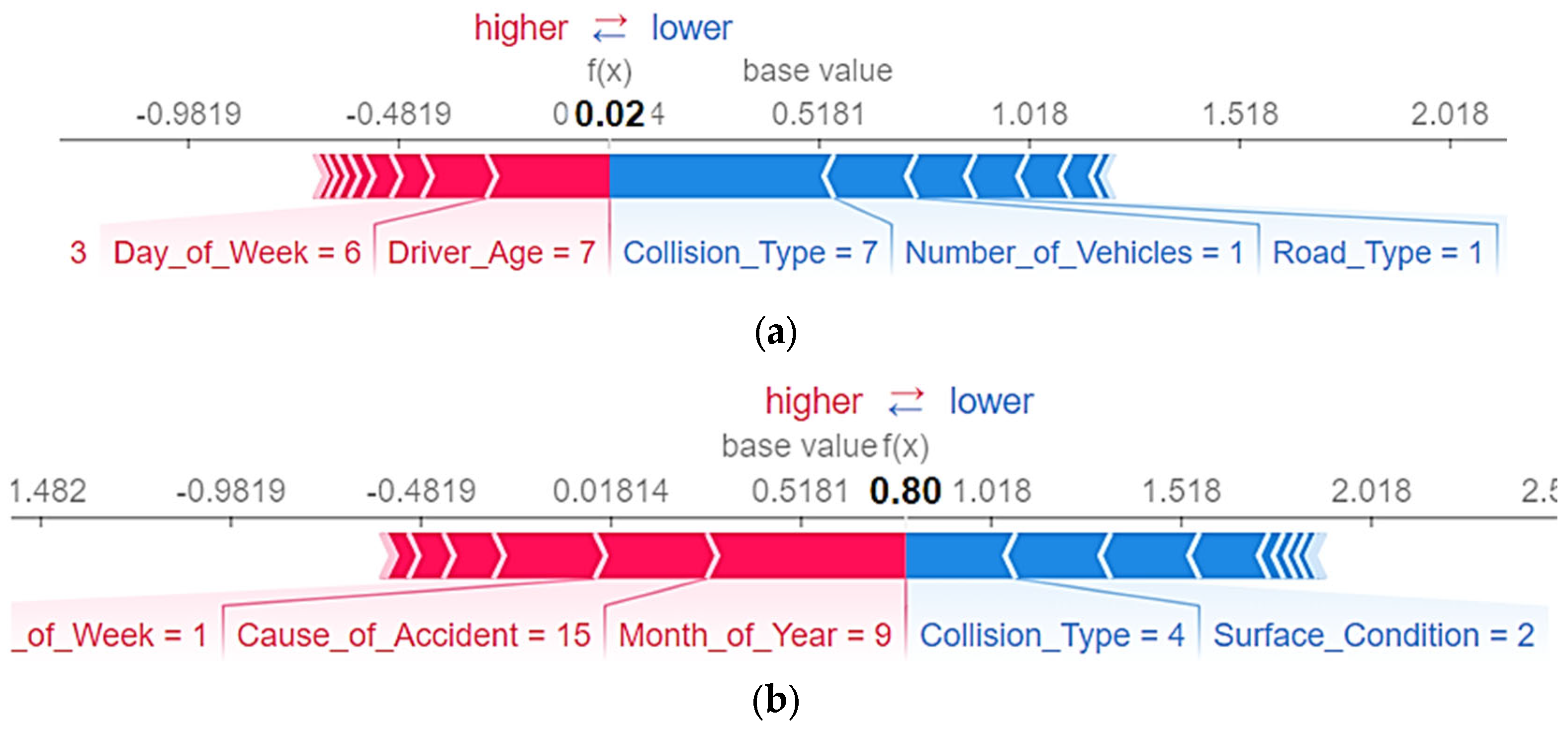
3.2.2. Local Variable Interpretation
3.2.3. Variable Interaction Analysis
4. Conclusions
Author Contributions
Funding
Institutional Review Board Statement
Informed Consent Statement
Data Availability Statement
Acknowledgments
Conflicts of Interest
References
- Chekijian, S.; Paul, M.; Kohl, V.P.; Walker, D.M.; Tomassoni, A.J.; Cone, D.C.; Vaca, F.E. The global burden of road injury: Its relevance to the emergency physician. Emerg. Med. Int. 2014, 2014, 139219. [Google Scholar] [CrossRef] [PubMed] [Green Version]
- NHTSA. 2015 motor vehicle crashes: Overview. Traffic Saf. Facts: Res. Note 2016, 2016, 1–9. [Google Scholar]
- Washington Annual Collision Summary 2015. Available online: https://www.wsdot.wa.gov/mapsdata/crash/pdf/2015_Annual_Collision_Summary.pdf (accessed on 20 November 2021).
- WHO. Global Status Report on Road Safety 2015 (Report No. 9789241565066). Available online: https://apps.who.int/iris/handle/10665/189242 (accessed on 24 November 2021).
- Hamim, O.F.; Hoque, M.S.; McIlroy, R.C.; Plant, K.L.; Stanton, N.A. A sociotechnical approach to accident analysis in a low-income setting: Using Accimaps to guide road safety recommendations in Bangladesh. Saf. Sci. 2020, 124, 104589. [Google Scholar] [CrossRef]
- Hussain, M.; Shi, J.; Batool, Z. An investigation of the effects of motorcycle-riding experience on aberrant driving behaviors and road traffic accidents-A case study of Pakistan. Int. J. Crashworthiness 2022, 27, 70–79. [Google Scholar] [CrossRef]
- Islam, M.A.; Dinar, Y. Evaluation and spatial analysis of road accidents in Bangladesh: An emerging and alarming issue. Transp. Dev. Econ. 2021, 7, 1–14. [Google Scholar] [CrossRef]
- Vipin, N.; Rahul, T. Road traffic accident mortality analysis based on time of occurrence: Evidence from Kerala, India. Clin. Epidemiol. Glob. Health 2021, 11, 100745. [Google Scholar]
- Zeng, Q.; Hao, W.; Lee, J.; Chen, F. Investigating the Impacts of Real-Time Weather Conditions on Freeway Crash Severity: A Bayesian Spatial Analysis. Int. J. Environ. Res. Public Health 2020, 17, 2768. [Google Scholar] [CrossRef] [PubMed]
- Ministry of Finance (G.o.P.). Pakistan Economic Survey 2015–16. Available online: https://www.finance.gov.pk/survey_1516.html (accessed on 18 October 2021).
- Ma, J.; Kockelman, K.M.; Damien, P. A multivariate Poisson-lognormal regression model for prediction of crash counts by severity, using Bayesian methods. Accid. Anal. Prev. 2008, 40, 964–975. [Google Scholar] [CrossRef] [Green Version]
- Aguero-Valverde, J.; Jovanis, P.P. Bayesian multivariate Poisson lognormal models for crash severity modeling and site ranking. Transp. Res. Rec. 2009, 2136, 82–91. [Google Scholar] [CrossRef]
- Nowakowska, M. Logistic models in crash severity classification based on road characteristics. Transp. Res. Rec. 2010, 2148, 16–26. [Google Scholar] [CrossRef]
- Pei, X.; Wong, S.; Sze, N.-N. A joint-probability approach to crash prediction models. Accid. Anal. Prev. 2011, 43, 1160–1166. [Google Scholar] [CrossRef] [PubMed]
- Haleem, K.; Abdel-Aty, M. Examining traffic crash injury severity at unsignalized intersections. J. Saf. Res. 2010, 41, 347–357. [Google Scholar] [CrossRef]
- Chen, F.; Chen, S. Injury severities of truck drivers in single-and multi-vehicle accidents on rural highways. Accid. Anal. Prev. 2011, 43, 1677–1688. [Google Scholar] [CrossRef] [PubMed]
- Chen, S.; Chen, F.; Wu, J. Multi-scale traffic safety and operational performance study of large trucks on mountainous interstate highway. Accid. Anal. Prev. 2011, 43, 429–438. [Google Scholar] [CrossRef] [PubMed]
- Ye, F.; Lord, D. Investigation of effects of underreporting crash data on three commonly used traffic crash severity models: Multinomial logit, ordered probit, and mixed logit. Transp. Res. Rec. 2011, 2241, 51–58. [Google Scholar] [CrossRef]
- Chen, F.; Ma, X.; Chen, S. Refined-scale panel data crash rate analysis using random-effects tobit model. Accid. Anal. Prev. 2014, 73, 323–332. [Google Scholar] [CrossRef]
- Xi, J.-F.; Liu, H.-Z.; Cheng, W.; Zhao, Z.-H.; Ding, T.-Q. The model of severity prediction of traffic crash on the curve. Math. Probl. Eng. 2014, 2014, 832723. [Google Scholar] [CrossRef] [Green Version]
- Ahmadi, A.; Jahangiri, A.; Berardi, V.; Machiani, S.G. Crash severity analysis of rear-end crashes in California using statistical and machine learning classification methods. J. Transp. Saf. Secur. 2020, 12, 522–546. [Google Scholar] [CrossRef]
- Chen, F.; Song, M.; Ma, X. Investigation on the injury severity of drivers in rear-end collisions between cars using a random parameters bivariate ordered probit model. Int. J. Environ. Res. Public Health 2019, 16, 2632. [Google Scholar] [CrossRef] [Green Version]
- Chen, F.; Ma, X.; Chen, S.; Yang, L. Crash frequency analysis using hurdle models with random effects considering short-term panel data. Int. J. Environ. Res. Public Health 2016, 13, 1043. [Google Scholar] [CrossRef] [Green Version]
- Chen, F.; Chen, S.; Ma, X. Crash frequency modeling using real-time environmental and traffic data and unbalanced panel data models. Int. J. Environ. Res. Public Health 2016, 13, 609. [Google Scholar] [CrossRef] [PubMed] [Green Version]
- Marzoug, R.; Lakouari, N.; Ez-Zahraouy, H.; Téllez, B.C.; Téllez, M.C.; Villalobos, L.C. Modeling and simulation of car accidents at a signalized intersection using cellular automata. Phys. A Stat. Mech. Appl. 2022, 589, 126599. [Google Scholar] [CrossRef]
- Alarifi, S.A.; Abdel-Aty, M.; Lee, J. A Bayesian multivariate hierarchical spatial joint model for predicting crash counts by crash type at intersections and segments along corridors. Accid. Anal. Prev. 2018, 119, 263–273. [Google Scholar] [CrossRef] [PubMed]
- Al-Moqri, T.; Haijun, X.; Namahoro, J.P.; Alfalahi, E.N.; Alwesabi, I. Exploiting Machine Learning Algorithms for Predicting Crash Injury Severity in Yemen: Hospital Case Study. Appl. Comput. Math. 2020, 9, 155–164. [Google Scholar] [CrossRef]
- Wen, X.; Xie, Y.; Wu, L.; Jiang, L. Quantifying and comparing the effects of key risk factors on various types of roadway segment crashes with LightGBM and SHAP. Accid. Anal. Prev. 2021, 159, 106261. [Google Scholar] [CrossRef]
- Tang, J.; Zheng, L.; Han, C.; Yin, W.; Zhang, Y.; Zou, Y.; Huang, H. Statistical and machine-learning methods for clearance time prediction of road incidents: A methodology review. Anal. Methods Accid. Res. 2020, 27, 100123. [Google Scholar] [CrossRef]
- Arteaga, C.; Paz, A.; Park, J. Injury severity on traffic crashes: A text mining with an interpretable machine-learning approach. Saf. Sci. 2020, 132, 104988. [Google Scholar] [CrossRef]
- Assi, K.; Rahman, S.M.; Mansoor, U.; Ratrout, N. Predicting crash injury severity with machine learning algorithm synergized with clustering technique: A promising protocol. Int. J. Environ. Res. Public Health 2020, 17, 5497. [Google Scholar] [CrossRef]
- Taamneh, S.; Taamneh, M.M. A machine learning approach for building an adaptive, real-time decision support system for emergency response to road traffic injuries. Int. J. Inj. Control. Saf. Promot. 2021, 28, 222–232. [Google Scholar] [CrossRef]
- Wahab, L.; Jiang, H. Severity prediction of motorcycle crashes with machine learning methods. Int. J. Crashworthiness 2020, 25, 485–492. [Google Scholar] [CrossRef]
- Yahaya, M.; Fan, W.; Fu, C.; Li, X.; Su, Y.; Jiang, X. A machine-learning method for improving crash injury severity analysis: A case study of work zone crashes in Cairo, Egypt. Int. J. Inj. Control. Saf. Promot. 2020, 27, 266–275. [Google Scholar] [CrossRef] [PubMed]
- Mohanta, B.K.; Jena, D.; Mohapatra, N.; Ramasubbareddy, S.; Rawal, B.S. Machine learning based accident prediction in secure iot enable transportation system. J. Intell. Fuzzy Syst. 2022, 42, 713–725. [Google Scholar] [CrossRef]
- Sangare, M.; Gupta, S.; Bouzefrane, S.; Banerjee, S.; Muhlethaler, P. Exploring the forecasting approach for road accidents: Analytical measures with hybrid machine learning. Expert Syst. Appl. 2021, 167, 113855. [Google Scholar] [CrossRef]
- Topuz, K.; Delen, D. A probabilistic Bayesian inference model to investigate injury severity in automobile crashes. Decis. Support. Syst. 2021, 113557. [Google Scholar] [CrossRef]
- Worachairungreung, M.; Ninsawat, S.; Witayangkurn, A.; Dailey, M.N. Identification of Road Traffic Injury Risk Prone Area Using Environmental Factors by Machine Learning Classification in Nonthaburi, Thailand. Sustainability 2021, 13, 3907. [Google Scholar] [CrossRef]
- Wu, P.; Meng, X.; Song, L. A novel ensemble learning method for crash prediction using road geometric alignments and traffic data. J. Transp. Saf. Secur. 2020, 12, 1128–1146. [Google Scholar] [CrossRef]
- Jiang, L.; Xie, Y.; Wen, X.; Ren, T. Modeling highly imbalanced crash severity data by ensemble methods and global sensitivity analysis. J. Transp. Saf. Secur. 2020, 1–23. [Google Scholar] [CrossRef]
- Peng, H.; Ma, X.; Chen, F. Examining Injury Severity of Pedestrians in Vehicle–Pedestrian Crashes at Mid-Blocks Using Path Analysis. Int. J. Environ. Res. Public Health 2020, 17, 6170. [Google Scholar] [CrossRef]
- Pham, B.T.; Nguyen-Thoi, T.; Qi, C.; Van Phong, T.; Dou, J.; Ho, L.S.; Van Le, H.; Prakash, I. Coupling RBF neural network with ensemble learning techniques for landslide susceptibility mapping. Catena 2020, 195, 104805. [Google Scholar] [CrossRef]
- Pandey, S.K.; Mishra, R.B.; Tripathi, A.K. BPDET: An effective software bug prediction model using deep representation and ensemble learning techniques. Expert Syst. Appl. 2020, 144, 113085. [Google Scholar] [CrossRef]
- Che, D.; Liu, Q.; Rasheed, K.; Tao, X. Decision tree and ensemble learning algorithms with their applications in bioinformatics. Softw. Tools Algorithms Biol. Syst. 2011, 696, 191–199. [Google Scholar]
- García-Herrero, S.; Gutiérrez, J.M.; Herrera, S.; Azimian, A.; Mariscal, M. Sensitivity analysis of driver’s behavior and psychophysical conditions. Saf. Sci. 2020, 125, 104586. [Google Scholar] [CrossRef]
- Jiang, L.; Xie, Y.; Ren, T. Modelling highly unbalanced crash injury severity data by ensemble methods and global sensitivity analysis. In Proceedings of the Transportation Research Board 98th Annual Meeting, Washington, DC, USA, 13–17 January 2019. [Google Scholar]
- Cattarin, G.; Pagliano, L.; Causone, F.; Kindinis, A.; Goia, F.; Carlucci, S.; Schlemminger, C. Empirical validation and local sensitivity analysis of a lumped-parameter thermal model of an outdoor test cell. Build. Environ. 2018, 130, 151–161. [Google Scholar] [CrossRef] [Green Version]
- Lundberg, S.M.; Lee, S.-I. A unified approach to interpreting model predictions. In Proceedings of the 31st international conference on neural information processing systems, Long Beach, CA, USA, 4–9 December 2017; pp. 4768–4777. [Google Scholar]
- Hu, J.; Huang, M.-C.; Yu, X. Efficient mapping of crash risk at intersections with connected vehicle data and deep learning models. Accid. Anal. Prev. 2020, 144, 105665. [Google Scholar] [CrossRef]
- Li, L.; Qiao, J.; Yu, G.; Wang, L.; Li, H.-Y.; Liao, C.; Zhu, Z. Interpretable tree-based ensemble model for predicting beach water quality. Water Res. 2022, 211, 118078. [Google Scholar] [CrossRef] [PubMed]
- Parsa, A.B.; Movahedi, A.; Taghipour, H.; Derrible, S.; Mohammadian, A.K. Toward safer highways, application of XGBoost and SHAP for real-time accident detection and feature analysis. Accid. Anal. Prev. 2020, 136, 105405. [Google Scholar] [CrossRef]
- Mangalathu, S.; Hwang, S.-H.; Jeon, J.-S. Failure mode and effects analysis of RC members based on machine-learning-based SHapley Additive exPlanations (SHAP) approach. Eng. Struct. 2020, 219, 110927. [Google Scholar] [CrossRef]
- Casado-Sanz, N.; Guirao, B.; Attard, M. Analysis of the risk factors affecting the severity of traffic accidents on Spanish crosstown roads: The driver’s perspective. Sustainability 2020, 12, 2237. [Google Scholar] [CrossRef] [Green Version]
- Duan, T.; Anand, A.; Ding, D.Y.; Thai, K.K.; Basu, S.; Ng, A.; Schuler, A. Ngboost: Natural gradient boosting for probabilistic prediction. In Proceedings of the International Conference on Machine Learning, 12–18 July 2020; pp. 2690–2700. [Google Scholar]
- Hancock, J.T.; Khoshgoftaar, T.M. CatBoost for big data: An interdisciplinary review. J. Big Data 2020, 7, 1–45. [Google Scholar] [CrossRef]
- Chen, T.; Xu, J.; Ying, H.; Chen, X.; Feng, R.; Fang, X.; Gao, H.; Wu, J. Prediction of extubation failure for intensive care unit patients using light gradient boosting machine. IEEE Access 2019, 7, 150960–150968. [Google Scholar] [CrossRef]
- Wang, F.; Jiang, D.; Wen, H.; Song, H. Adaboost-based security level classification of mobile intelligent terminals. J. Supercomput. 2019, 75, 7460–7478. [Google Scholar] [CrossRef]
- Kavzoglu, T.; Teke, A. Predictive Performances of Ensemble Machine Learning Algorithms in Landslide Susceptibility Mapping Using Random Forest, Extreme Gradient Boosting (XGBoost) and Natural Gradient Boosting (NGBoost). Arab. J. Sci. Eng. 2022, 1–19. [Google Scholar] [CrossRef]
- Yuan, Z.; Zhou, T.; Liu, J.; Zhang, C.; Liu, Y. Fault Diagnosis Approach for Rotating Machinery Based on Feature Importance Ranking and Selection. Shock Vib. 2021, 2021, 8899188. [Google Scholar] [CrossRef]
- Liang, S.; Peng, J.; Xu, Y.; Ye, H. Passive Fetal Movement Recognition Approaches Using Hyperparameter Tuned LightGBM Model and Bayesian Optimization. Comput. Intell. Neurosci. 2021, 2021, 6252362. [Google Scholar] [CrossRef] [PubMed]
- Xia, Y.; Liu, C.; Li, Y.; Liu, N. A boosted decision tree approach using Bayesian hyper-parameter optimization for credit scoring. Expert Syst. Appl. 2017, 78, 225–241. [Google Scholar] [CrossRef]
- Turner, R.; Eriksson, D.; McCourt, M.; Kiili, J.; Laaksonen, E.; Xu, Z.; Guyon, I. Bayesian optimization is superior to random search for machine learning hyperparameter tuning: Analysis of the black-box optimization challenge 2020. arXiv 2021, arXiv:2104.10201. [Google Scholar]
- Brownlee, J. Machine Learning Algorithms from Scratch with Python; Machine Learning Mastery: San Francisco, CA, USA, 2016. [Google Scholar]
- Sun, F.; Dubey, A.; White, J. DxNAT—Deep neural networks for explaining non-recurring traffic congestion. In Proceedings of the 2017 IEEE International Conference on Big Data (Big Data), Boston, MA, USA, 11–14 December 2017; pp. 2141–2150. [Google Scholar]
- Merrick, L.; Taly, A. The explanation game: Explaining machine learning models with cooperative game theory. arXiv 2019, arXiv:1909.08128. [Google Scholar]
- Shaik, M.E.; Islam, M.M.; Hossain, Q.S. A review on neural network techniques for the prediction of road traffic accident severity. Asian Transp. Stud. 2021, 7, 100040. [Google Scholar] [CrossRef]
- Mujalli, R.O.; Oña, J.d. Injury severity models for motor vehicle accidents: A review. Proc. Inst. Civ. Eng. Transp. 2013, 166, 255–270. [Google Scholar] [CrossRef]
- Kang, K.; Ryu, H. Predicting types of occupational accidents at construction sites in Korea using random forest model. Saf. Sci. 2019, 120, 226–236. [Google Scholar] [CrossRef]
- Zhang, C.; He, J.; Wang, Y.; Yan, X.; Zhang, C.; Chen, Y.; Liu, Z.; Zhou, B. A crash severity prediction method based on improved neural network and factor Analysis. Discret. Dyn. Nat. Soc. 2020, 2020, 4013185. [Google Scholar] [CrossRef]
- Al Reesi, H.; Al Maniri, A.; Adawi, S.A.; Davey, J.; Armstrong, K.; Edwards, J. Prevalence and characteristics of road traffic injuries among young drivers in Oman, 2009–2011. Traffic Inj. Prev. 2016, 17, 480–487. [Google Scholar] [CrossRef] [PubMed] [Green Version]
- Donmez, B.; Liu, Z. Associations of distraction involvement and age with driver injury severities. J. Saf. Res. 2015, 52, 23–28. [Google Scholar] [CrossRef] [PubMed]
- Behnood, A.; Al-Bdairi, N.S.S. Determinant of injury severities in large truck crashes: A weekly instability analysis. Saf. Sci. 2020, 131, 104911. [Google Scholar] [CrossRef]
- Ullah, H.; Farooq, A.; Shah, A.A. An Empirical Assessment of Factors Influencing Injury Severities of Motor Vehicle Crashes on National Highways of Pakistan. J. Adv. Transp. 2021, 2021, 6358321. [Google Scholar] [CrossRef]
- Hao, W.; Kamga, C.; Wan, D. The effect of time of day on driver’s injury severity at highway-rail grade crossings in the United States. J. Traffic Transp. Eng. 2016, 3, 37–50. [Google Scholar] [CrossRef] [Green Version]


| Variables | EU Directive | USA | Australia | New Zealand | Pakistan |
|---|---|---|---|---|---|
| Crash Location | Precise as possible location | Road name, GPS coordinates | Road name, reference point, distance, direction | Road name, GPS coordinates | District and kilometer marker no. starting from Karachi city (00) |
| Crash Narrative | No | No | Yes | No | No |
| Crash Sketch | No | No | Yes, restricted access | Yes | No |
| Crash Type | Yes | Recorded in the traffic units Section | Yes | Yes | Yes |
| Collision Type | Yes | 8 descriptors | Yes | Yes | Yes |
| Contributing Circumstances | No | Environmental circumstances | Yes | Yes | Yes |
| Weather Conditions | Yes | 10 descriptors | Yes | 5 descriptors | 3 descriptors |
| Lighting Condition | Yes | 7 descriptors | Yes | 7 descriptors | 3 descriptors |
| Reported Crashes | Not specified | All severities | All injury severities | All severities | All severities |
| Definition Non-fatal Injury Levels | Severe and non-severe injuries | Suspected serious injury, suspected minor injury, possible injury | Injured, admitted to hospital injured, required medical treatment | Major and minor injuries | Fatal injury, major injury, minor injury, and no injury |
| Contributing Circumstances | No | 11 descriptors | No | Numerous causes | Yes |
| Speed Limit | Yes | Yes | Yes | Yes | No |
| Surface Conditions | Yes | 10 descriptors | Yes | 3 descriptors | Yes |
| Road Curves | No | Yes | Yes | 4 descriptors | Yes |
| Gradient | No | Yes | No | No | No |
| Age | Yes | Date of birth | Yes | Yes | Yes |
| Gender | Yes | Yes | Yes | Yes | Yes |
| Nationality | Yes | No | Foreign drivers’ identification | Foreign drivers’ identification | No |
| Alcohol Level | Yes | Yes | Yes | Yes | No |
| Drug Test Results | No | Yes | Yes | Yes | No |
| Safety Equipment | Yes | Yes | Yes | Yes | No |
| Curve Radius | No | Yes | Yes | Yes | No |
| Curve Length | No | Yes | Yes | Yes | No |
| Type of Variable | Variable | Description | Marginal Frequency (%) |
|---|---|---|---|
| Injury Severity | Injury Severity Category | Fatal/Non-Fatal | 38.09/61.91 |
| Vehicle Specific | Type_of_Vehicle | Rickshaw/Motorcycle/Bicycle/ Car/Pickup/Minibus/Bus/Truck/ Dumper/Trailer/Tractor | 5.34/6.78/10.77/ 12.69/3.50/9.19/8.48/ 20.08/4.43/16.44/2.30 |
| Vehicle_Age (years) | 0–10/11–20/21–30/31–40/41+ | 32.01/36.49/15.30/9.30/6.90 | |
| Number_of_Vehicles (Number of vehicles in crash) | Single/Multiple | 33.46/66.54 | |
| Driver Specific | Driver Gender | Female/Male | 0.001/99.99 |
| Driver_Age (Years) | 18–25/26–30/31–35/36–40/41–45/46–50/51–55/55+ | 18.18/16.83/14.90/14.58/ 13.62/10.92/5.84/5.14 | |
| Driving_License | No/Yes | 46.52/53.48 | |
| Environment Specific | Lighting_Condition | Daylight/Night with Road Lights/Night without Road Lights | 69.11/5.33/25.56 |
| Weather_Condition | Sunny/Cloudy/Rainy | 89.85/3.59/6.56 | |
| Visibility_Condition | Clear/Fog/Smog | 96.41/3.08/0.50 | |
| Temporal Specific | Month_of_Year | January/February/March/ April/May/June/July/August/ September/October/November/ December | 5.65/6.29/10.08/8.73/5.27/ 6.87/14.96/10.08/13.17/ 6.10/7.32/5.46 |
| Day_of_Week | Monday/Tuesday/Wednesday/ Thursday/Friday/Saturday/Sunday | 10.76/12.67/14.52/13.51/16.87/ 16.82/14.85 | |
| Time_of_Day | 12:00:00 a.m.–3:59:59 a.m./4:00:00 a.m.–7:59:59 a.m./8:00:00 a.m.–11:59:59 p.m./12:00:00 p.m.–3:59:59 p.m./4:00:00 p.m.–7:59:59 p.m./8:00:00 p.m.–11:59:59 p.m. | 8.97/14.41/23.09/21.13/ 21.02/11.38 | |
| Type_of_Day | Weekday/Weekend | 68.22/31.78 | |
| Roadway Specific | Alignment | Straight/Horizontal Curve/Vertical Curve/Both Horizontal and Vertical Curves | 84.36/5.66/4.43/5.55 |
| Presence_of_Shoulder | No/Yes | 2.63/97.37 | |
| Surface_Condition | Dry/Wet | 92.49/7.51 | |
| Pavement_Roughness | Smooth/Rough/Potholes | 94.23/2.52/3.25 | |
| Road_Type | Urban/Rural | 52.86/47.14 | |
| Presence_of_Median | No/Yes | 3.64/96.36 | |
| Work_Zone | No/Yes | 98.64/1.35 | |
| Crash Specific | Collision_Type | Head on Collision/Rear End Collision/Side Collision/Rollover/ Skidding/Hit Obstacle on Road/Hit Pedestrian/Hit Animal/Run off Roadway/Hitting Nearby Trees/Fell off Bridge | 5.21/43.55/19.17/12.44/ 3.08/4.88/10.31/0.28/ 0.78/0.11/0.17 |
| Cause_of_Accident | Bicycle Rider at-Fault/Wrong Side Overtaking/Pedestrian at-Fault/Pavement Distress/Driver at-Fault/Dozing at the Wheel/Over Speeding/Motorcycle Rider at-Fault/Low Visibility/Mechanical Fault of Vehicle/Sight Obstruction/Slippery Road/Vehicle out of Control/Other | 0.56/1.46/7.29/1.51/56.331.40/3.87/3.14/0.39/7.74/ 1.79/2.35/0.90/2.35/8.91 |
| Algorithm | Evaluation Metric | Hyperparameters | Range | Optimal Values |
|---|---|---|---|---|
| CatBoost | Classification accuracy | n_estimators | (100, 5000) | 11,600 |
| max_depth | (0, 10) | 5 | ||
| learning_rate | (0.001, 0.5) | 0.002 | ||
| LightGBM | Classification accuracy | n_estimators | (100, 5000) | 3300 |
| learning_rate | (0.001, 0.5) | 0.042 | ||
| max_depth | (0, 10) | 6 | ||
| lambda_l1 | (1 × 10⁻⁸, 10) | 0.52 | ||
| lambda_l2 | (1 × 10⁻⁸, 10) | 0.2 | ||
| NGBoost | Classification accuracy | learning_rate | (0.001, 0.50) | 0.01 |
| n_estimators | (100, 5000) | 600 | ||
| Max_depth | (0, 10) | 4 | ||
| AdaBoost | Classification accuracy | n_estimators | (100–5000) | 800 |
| Learning_rate | (0.01, 1) | 0.5 |
| Performance Metrics | Proposed Boosting-Based Ensemble Models | Existing Models for Road Traffic Injury Severity | ||||
|---|---|---|---|---|---|---|
| CatBoost | LightGBM | NGBoost | AdaBoost | ANN [66] | Logit Model [67] | |
| Accuracy (%) | 67.34 | 73.63 | 61.13 | 66.87 | 62.17 | 60.47 |
| Precision (%) | 67.32 | 72.61 | 61.33 | 61.21 | 62.37 | 88.71 |
| Recall (%) | 55.87 | 70.09 | 54.71 | 59.17 | 60.60 | 63.10 |
| F1—Score (%) | 51.28 | 70.81 | 49.04 | 60.11 | 50.81 | 50.81 |
| AUC | 0.684 | 0.713 | 0.588 | 0.619 | 0.601 | 0.533 |
Publisher’s Note: MDPI stays neutral with regard to jurisdictional claims in published maps and institutional affiliations. |
© 2022 by the authors. Licensee MDPI, Basel, Switzerland. This article is an open access article distributed under the terms and conditions of the Creative Commons Attribution (CC BY) license (https://creativecommons.org/licenses/by/4.0/).
Share and Cite
Dong, S.; Khattak, A.; Ullah, I.; Zhou, J.; Hussain, A. Predicting and Analyzing Road Traffic Injury Severity Using Boosting-Based Ensemble Learning Models with SHAPley Additive exPlanations. Int. J. Environ. Res. Public Health 2022, 19, 2925. https://doi.org/10.3390/ijerph19052925
Dong S, Khattak A, Ullah I, Zhou J, Hussain A. Predicting and Analyzing Road Traffic Injury Severity Using Boosting-Based Ensemble Learning Models with SHAPley Additive exPlanations. International Journal of Environmental Research and Public Health. 2022; 19(5):2925. https://doi.org/10.3390/ijerph19052925
Chicago/Turabian StyleDong, Sheng, Afaq Khattak, Irfan Ullah, Jibiao Zhou, and Arshad Hussain. 2022. "Predicting and Analyzing Road Traffic Injury Severity Using Boosting-Based Ensemble Learning Models with SHAPley Additive exPlanations" International Journal of Environmental Research and Public Health 19, no. 5: 2925. https://doi.org/10.3390/ijerph19052925
APA StyleDong, S., Khattak, A., Ullah, I., Zhou, J., & Hussain, A. (2022). Predicting and Analyzing Road Traffic Injury Severity Using Boosting-Based Ensemble Learning Models with SHAPley Additive exPlanations. International Journal of Environmental Research and Public Health, 19(5), 2925. https://doi.org/10.3390/ijerph19052925