
Risk Assessment Matrices for Workplace Hazards: Design for Usability


Abstract
:1. Introduction
1.1. Background on Risk Assessment
1.2. Diverse Options for Design
1.3. Usability Issues
- Improbable and seldom.
- Often, frequent, and probable.
- Disastrous and catastrophic.
1.4. Reasons for a Second Survey
2. Materials and Methods
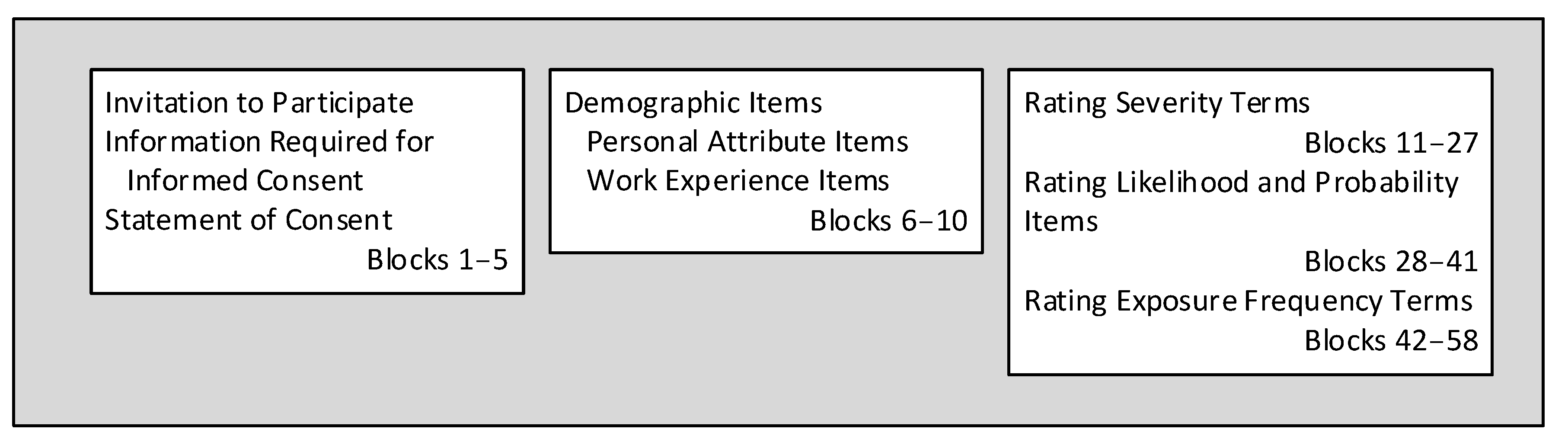
2.1. The Survey Instrument
- For rating severity terms, the end points were No harm and Worst harm.
- For likelihood and probability terms, the end points were Impossible and Certain.
- For extent of exposure terms, the end points were No exposure and Constant exposure.
2.2. Rationale for Terms Included in the Survey
2.3. Procedures
3. Results
3.1. Demographics of Respondents
3.2. Ratings of Terms in Present Survey
3.3. Parallel Wording
- Extremely improbable and extremely unlikely: (median 6, 7|mean 15.2, 15.9).
- Somewhat improbable and somewhat unlikely: (median 22, 25.5|mean 28.5, 24.8).
- Moderately probable and moderately likely: (median 57.5, 55|mean 61.1, 56.9).
- Probable and likely: (median 67, 65|mean 65.3, 67.2).
- Highly probable and highly likely: (median 88.5, 81|mean 87.1, 84.2).
- Improbable and unlikely: (median 10, 20|mean 14.1, 20.8).
- Somewhat probable and somewhat likely: (median 56, 40|mean 57.2, 45.6).
3.4. Rating from Two Surveys Compared
4. Discussion
4.1. Selectively Removing Terms
4.2. Calendar-Based Terms
4.3. Limitations
5. Recommendations
6. Conclusions
- The survey confirmed the prior recommendations for severity terms. However, the authors recommend limiting use of the set containing the word “damage” to hazards concerned with harm to equipment, facilities, products and the environment.
- The survey confirmed the prior recommendations for likelihood terms with some suggestions. The term somewhat likely had a median in this survey of 40, but a median of 60 in the prior survey. That does not negate use of the term, but due to the inconsistent ratings, we suggest using moderately likely with a median rating of 55.
- Based on ratings in both surveys, the ratings for the terms for the lowest likelihood category did not produce a winner. Three terms intended for naming the lowest category, with their medians, are: very unlikely (11), extremely unlikely (7), or highly unlikely (10). We express no preference.
- The survey found concerns with some terms in the probability sets. The prior survey did not include terms with rating in the middle range of probability, so four terms were added to the survey: fairly normal, moderately, somewhat probable, and somewhat improbable. Rating for these terms provides alternatives for the word occasionally in the sets found in Table 16. The authors recommend replacing occasionally in the upper set with fairly normal, and in the three lower sets with somewhat improbable.
- The survey confirmed the prior recommendations for extent of exposure with small changes. An improvement incorporated into the present survey was adding the word “exposed” to four words in the prior survey to make four terms—regularly exposed, occasionally exposed, seldom exposed, and rarely exposed.
Supplementary Materials
Author Contributions
Funding
Institutional Review Board Statement
Informed Consent Statement
Data Availability Statement
Conflicts of Interest
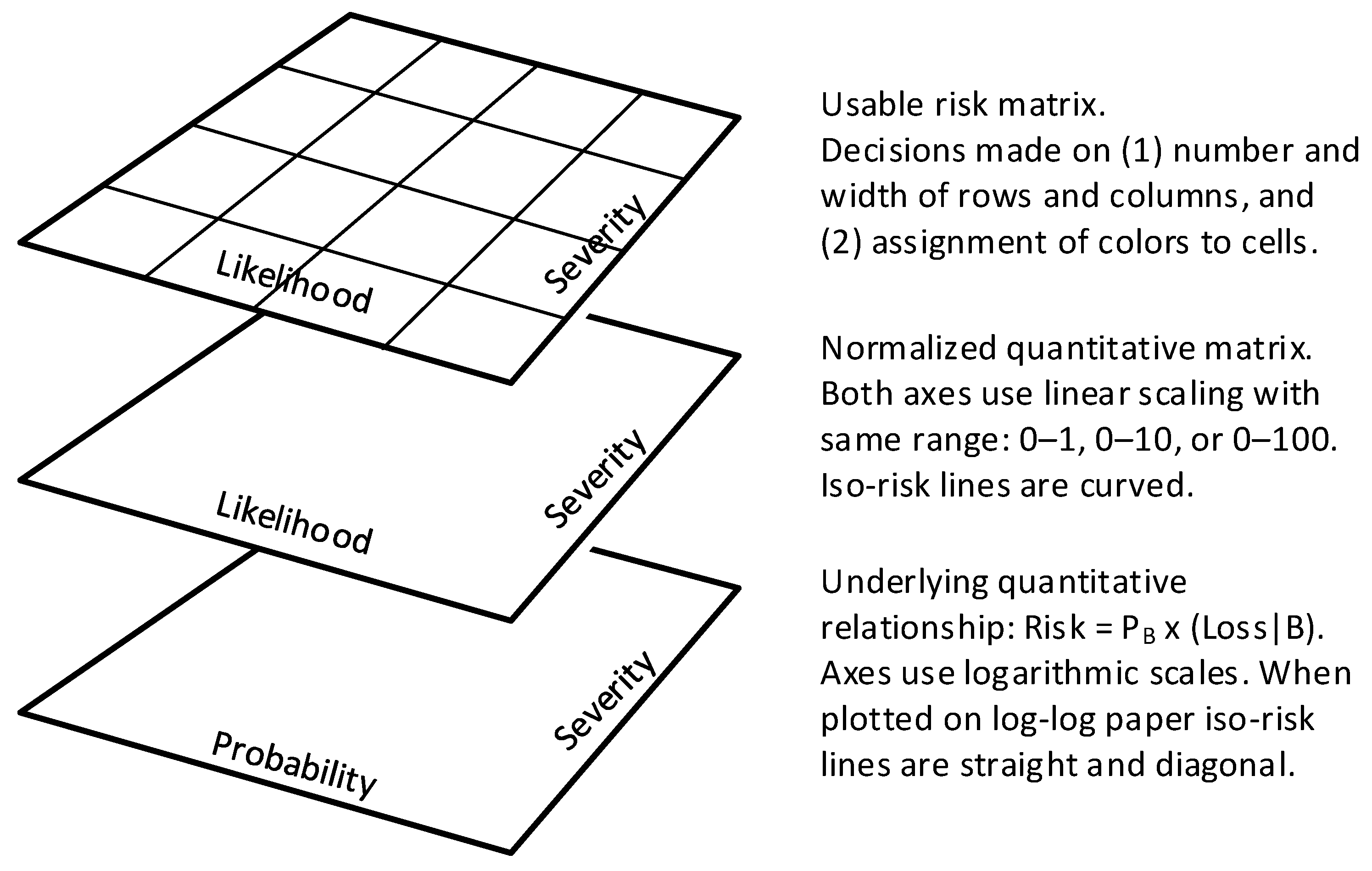
Appendix A. Rationale for Normalized, Equal-Axis Risk Matrices

References
- Friend, M.A.; Zontek, T.L.; Ogle, B.R. Planning and Managing Safety: A History. In Planning and Managing the Safety System; Friend, M.W., Ed.; Bernham: Lanham, MD, USA, 2017; pp. 1–16. [Google Scholar]
- Jensen, R.C. Risk-Reduction Methods for Occupational Safety and Health, 2nd ed.; Wiley: Hoboken, NJ, USA, 2019; pp. 65–81. ISBN 978-1-1194-9399-0. [Google Scholar]
- Kjellén, U.; Albrechtsen, E. Prevention of Accidents and Unwanted Occurrences: Theory, Methods, and Tools in Safety Management, 2nd ed.; CRC: Boca Raton, FL, USA, 2017; pp. 1–7, 339–351. ISBN 978-1-4987-3659-6. [Google Scholar]
- ISO, 45001; Occupational Health and Management Systems—Requirements with Guidance for Use, 2018 ed. International Organisation for Standardization: Geneva, Switzerland, 2018.
- Main, B.W. Risk assessment: A review of the fundamental principles. Prof. Saf. 2004, 49, 37–47. [Google Scholar]
- Rausand, M. Risk Assessment: Theory, Methods, and Applications; Wiley: Hoboken, NJ, USA, 2011; pp. 99–102. ISBN 978-1-4398-0684-5. [Google Scholar]
- Pawlowska, Z. Occupational risk assessment. In Handbook of Occupational Safety and Health; Koradecka, D., Ed.; CRC: Boca Raton, FL, USA, 2010; pp. 473–481. ISBN 978-1-4398-0684-5. [Google Scholar]
- Baybutt, P. Guidelines for designing risk matrices. Process Saf. Prog. 2018, 37, 49–55. [Google Scholar] [CrossRef]
- Ale, B.; Burnap, P.; Slater, D. On the origin of PDCS—(Probability consequence diagrams). Saf. Sci. 2015, 72, 229–239. [Google Scholar] [CrossRef]
- Baybutt, P. Calibration of risk matrices for process safety. J. Loss Prev. Process Ind. 2015, 38, 163–168. [Google Scholar] [CrossRef]
- Duijm, N.J. Recommendations on the use and design of risk matrices. Saf. Sci. 2015, 76, 21–31. [Google Scholar] [CrossRef] [Green Version]
- Ball, D.J.; Watt, J. Further thoughts on the utility of risk matrices. Risk Anal. 2013, 33, 2068–2078. [Google Scholar] [CrossRef] [PubMed]
- Cox, L.A., Jr. What’s wrong with risk matrices? Risk Anal. 2008, 28, 497–512. [Google Scholar] [CrossRef] [PubMed]
- Bao, C.; Wu, D.; Wan, J.; Li, J.; Chen, J. Comparison of different methods to design risk matrices from the perspective of applicability. Procedia Comput. Sci. 2017, 122, 455–462. [Google Scholar] [CrossRef]
- Pons, D.J. Alignment of the safety method with New Zealand legislative responsibilities. Safety 2019, 5, 59. [Google Scholar] [CrossRef] [Green Version]
- Aven, T. Improving risk characterisations in practical situations by highlighting knowledge aspects, with applications to risk matrices. Reliab. Eng. Syst. Saf. 2017, 17, 42–48. [Google Scholar] [CrossRef]
- Cox, L.A., Jr.; Babayev, D.; Huber, W. Some limitations of qualitative risk rating systems. Risk Anal. 2005, 25, 651–662. [Google Scholar] [CrossRef] [PubMed]
- Goerlandt, F.; Reniers, G. On the assessment of uncertainty in risk diagrams. Saf. Sci. 2016, 84, 67–77. [Google Scholar] [CrossRef]
- Card, A.J.; Ward, J.R.; Clarkson, J. Trust-level risk evaluation and risk control guidance in the NHS east of England. Risk Anal. 2014, 34, 1469–1481. [Google Scholar] [CrossRef] [PubMed]
- Kaya, G.K.; Ward, J.; Clarkson, J. A review of risk matrices used in acute hospitals in England. Risk Anal. 2019, 39, 1060–1070. [Google Scholar] [CrossRef] [PubMed]
- Jensen, R.C.; Hansen, H. Selecting appropriate words for naming the rows and columns of risk assessment matrices. Int. J. Environ. Res. Public Health 2020, 17, 5521. [Google Scholar] [CrossRef] [PubMed]
- U.S. Department of Defense. MIL-STD-882E, Standard Practice for System Safety. p. 12. Available online: www.system-safety.org/Documents/MIL=STD-882E.pdf. (accessed on 28 December 2019).
- Hamka, M.A. Safety risk assessment on container terminal using hazard identification and risk assessment and fault tree analysis methods. Procedia Manuf. 2017, 194, 307–314. [Google Scholar]
- Ruan, X.; Yin, Z.; Frangopol, D.M. Risk matrix integrating risk attitudes based on utility theory. Risk Anal. 2015, 35, 1437–1447. [Google Scholar] [CrossRef] [PubMed]
- Minitab Inc. Minitab Statistical Software, Version 19; Minitab Inc.: State College, PA, USA, 2020. [Google Scholar]


| Axis Parameter | Number of Categories | Number of Sets Recommended | Example |
|---|---|---|---|
| Severity | Three | 3 | |
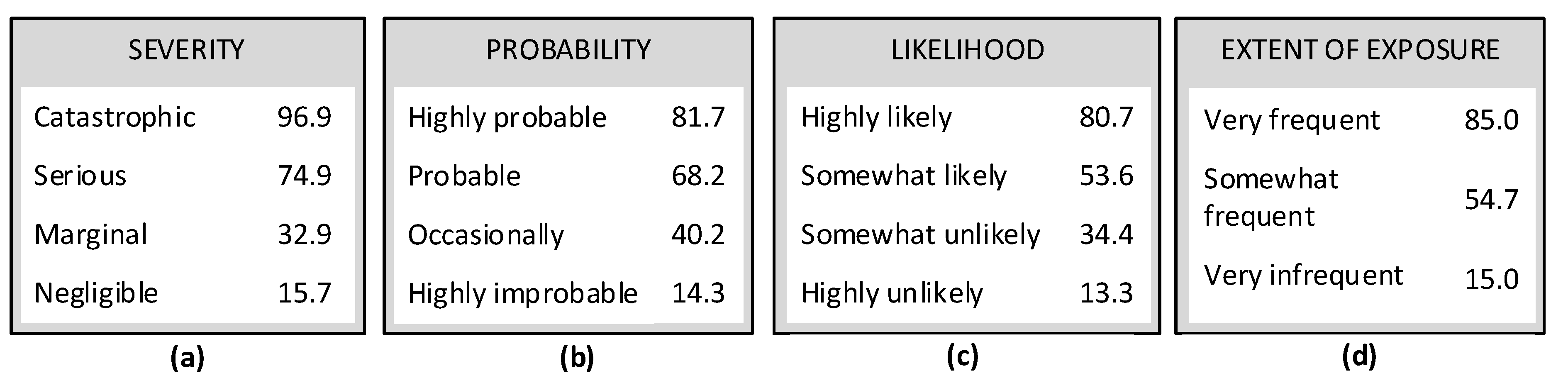
| Four | 1 | Figure 4a | |
| Five | 2 | ||
| Probability | Three | 1 | |
| Four | 1 | Figure 4b | |
| Five | 1 | ||
| Six | 1 | ||
| Likelihood | Three | 1 | |
| Four | 1 | Figure 4c | |
| Five | 1 | ||
| Six | 1 | ||
| Extent of Exposure | Two | 1 | |
| Three | 2 | Figure 4d |
| Probability Terms | Likelihood Terms | ||||
|---|---|---|---|---|---|
| Term Studied | Same | Different | Term Studied | Same | Different |
| Highly probable | X | Highly likely | X | ||
| Probable | X | Likely | X | ||
| Improbable | X | Somewhat likely | X | ||
| Remote | X | Somewhat unlikely | X | ||
| Fairly normal | X | Unlikely | X | ||
| Moderately probable | X | Certain | X | ||
| Extremely probable | X | Almost certain | X | ||
| Extremely improbable | X | Extremely unlikely | X | ||
| Somewhat probable | X | Extremely likely | X | ||
| Somewhat improbable | X | Moderately likely | X | ||
| Fairly normal | X | ||||
| Very unlikely | X | ||||
| Very likely | X | ||||
| Severity Terms | Extent of Exposure Terms | ||
|---|---|---|---|
| Current Study Term | Prior Study | Current Study Terms | Prior Study Terms |
| Catastrophic | Same | Very frequently | Very frequent |
| Medical treatment case | Same | Frequently | Frequent |
| Severe | Same | Somewhat frequently | Somewhat frequent |
| Moderate | Same | Infrequently | Infrequent |
| Minor damage | Same | Very infrequently | Very infrequent |
| Insignificant | Same | — | — |
| Serious | Same | Regularly exposed | Regularly |
| Severe loss | Same | Occasionally exposed | Occasionally |
| Major damage | Same | Seldom exposed | Seldom |
| Negligible | Same | Rarely exposed | Rarely |
| Permanent injury/illness | Same | — | — |
| Critical | Same | Annually | Same |
| Minor | Same | Monthly | Same |
| Death of a person 1 | Same | Weekly | Same |
| First aid only case | Same | Daily | Same |
| Marginal | Same | ||
| Age | N | Prct. | Gender | N | Prct. | Ethnicity or Race | N | Prct. |
|---|---|---|---|---|---|---|---|---|
| 60–69 | 1 | 02.7 | Male | 25 | 69.4 | White/Caucasian | 27 | 75.0 |
| 50–59 | 5 | 13.5 | Female | 11 | 30.6 | Hispanic/Latinx | 4 | 11.1 |
| 40–49 | 11 | 29.7 | Decline | 1 | NA | Asian | 3 | 8.3 |
| 30–39 | 12 | 32.4 | Native American 1 | 1 | 2.8 | |||
| 20–29 | 8 | 21.6 | Other (African) | 1 | 2.8 | |||
| Total | 37 | 99.9 2 | 37 | 100.0 | 36 | 100.0 |
| Most Experience | N | Prct. | Sector Employed | N | Prct. |
|---|---|---|---|---|---|
| Occupational Safety | 5 | 13.5 | Private Industrial | 9 | 25.0 |
| Industrial Hygiene | 12 | 32.4 | Private Commercial | 5 | 13.9 |
| Occupational S&H Combined | 12 | 32.4 | Education | 4 | 11.1 |
| Environmental Protection | 6 | 16.2 | Federal Military | 3 | 8.3 |
| Responder | 1 | 2.7 | Federal Non-Military | 7 | 19.4 |
| Other (not specified) | 1 | 2.7 | Non-Federal Government | 7 | 19.4 |
| Other | 1 | 2.8 | |||
| Total | 37 | 99.9 1 | Total | 36 | 99.9 1 |
| Term Rated | N | Mean | St. Dev. | Median |
|---|---|---|---|---|
| Death of a person 1 | 32 | 99.7 | 1.4 | 100.0 |
| Catastrophic | 33 | 96.4 | 6.5 | 100.0 |
| Permanent Injury/Illness | 33 | 87.3 | 18.9 | 92.0 |
| Severe Loss | 34 | 77.1 | 11.8 | 85.0 |
| Critical | 34 | 78.9 | 13.4 | 81.0 |
| Severe | 34 | 77.1 | 11.8 | 80.0 |
| Serious | 34 | 71.0 | 13.8 | 70.0 |
| Major Damage | 30 | 71.3 | 17.0 | 70.5 |
| Medical Treatment Case | 34 | 57.4 | 19.1 | 60.0 |
| Moderate | 34 | 44.9 | 12.6 | 50.0 |
| First Aid Only Case | 34 | 25.9 | 16.4 | 24.5 |
| Marginal | 33 | 26.4 | 12.8 | 21.0 |
| Minor Damage | 33 | 22.9 | 8.7 | 20.0 |
| Minor | 33 | 20.6 | 10.1 | 20.0 |
| Negligible | 29 | 21.3 | 26.0 | 10.0 |
| Insignificant | 26 | 10.5 | 16.5 | 5.5 |
| Term Rated | N | Mean | St. Dev. | Median |
|---|---|---|---|---|
| Certain | 31 | 95.1 | 12.4 | 100.0 |
| Extremely Probable | 31 | 93.9 | 4.9 | 95.0 |
| Almost Certain | 33 | 92.1 | 7.0 | 94.0 |
| Highly Probable | 30 | 87.8 | 7.9 | 88.5 |
| Probable | 31 | 65.4 | 16.8 | 67.0 |
| Moderately Probable | 30 | 61.1 | 14.2 | 57.5 |
| Somewhat Probable | 28 | 57.3 | 15.0 | 56.0 |
| Fairly Normal | 31 | 53.5 | 22.7 | 51.0 |
| Somewhat Improbable | 31 | 28.5 | 14.2 | 22.0 |
| Remote | 30 | 25.1 | 22.4 | 16.5 |
| Improbable | 27 | 14.1 | 9.3 | 10.0 |
| Extremely Improbable | 25 | 15.2 | 24.9 | 6.0 |
| Term Rated | N | Mean | St. Dev. | Median |
|---|---|---|---|---|
| Certain | 31 | 95.1 | 12.4 | 100.0 |
| Almost Certain | 33 | 92.1 | 7.0 | 94.0 |
| Extremely Likely | 30 | 87.0 | 16.4 | 90.0 |
| Highly Likely | 31 | 84.2 | 9.4 | 81.0 |
| Likely | 31 | 67.2 | 16.9 | 65.0 |
| Moderately Likely | 31 | 56.9 | 12.5 | 55.0 |
| Fairly Normal | 31 | 53.5 | 22.7 | 51.0 |
| Somewhat Likely | 31 | 45.5 | 16.4 | 40.0 |
| Somewhat Unlikely | 32 | 24.8 | 13.0 | 25.5 |
| Unlikely | 27 | 20.8 | 12.3 | 20.0 |
| Remote | 30 | 25.1 | 22.4 | 16.5 |
| Extremely Unlikely | 28 | 15.9 | 26.7 | 7.0 |
| Term Rated | N | Mean | St. Dev. | Median |
|---|---|---|---|---|
| Daily 1 | 30 | 90.1 | 12.2 | 94.0 |
| Very Frequently | 31 | 80.8 | 17.0 | 82.0 |
| Regularly Exposed | 30 | 75.1 | 18.7 | 77.5 |
| Frequently | 31 | 72.7 | 16.2 | 75.0 |
| Weekly 1 | 30 | 64.6 | 21.4 | 70.5 |
| Somewhat Frequently | 31 | 56.7 | 16.2 | 60.0 |
| Monthly 1 | 31 | 42.4 | 18.3 | 44.0 |
| Occasionally exposed | 31 | 39.2 | 24.8 | 31.0 |
| Somewhat Infrequently | 31 | 30.1 | 17.6 | 27.0 |
| Infrequently | 30 | 22.2 | 16.1 | 20.5 |
| Annually 1 | 30 | 21.9 | 17.7 | 19.0 |
| Seldom Exposed | 31 | 17.4 | 19.3 | 11.0 |
| Very Infrequently | 29 | 14.7 | 21.0 | 10.0 |
| Rarely Exposed | 25 | 9.6 | 11.4 | 6.0 |
| Terms for Severity of Harm | Previous Survey: Undergraduates | Present Survey: Experienced | ∆ Medians 1 | % Diff 2 | ||
|---|---|---|---|---|---|---|
| Mean | Median | Mean | Median | |||
| Minor | 21.8 | 20 | 20.6 | 20 | 0.0 | 0.0 |
| Catastrophic | 96.8 | 100 | 96.4 | 100 | 0.0 | 0.0 |
| Minor damage | 25.0 | 20 | 22.3 | 20 | 0.0 | 0.0 |
| Negligible | 15.7 | 10 | 21.3 | 10 | 0.0 | 0.0 |
| Moderate | 48.9 | 50 | 44.9 | 50 | 0.0 | 0.0 |
| Death of one person 3 | 97.1 | 100 | 99.8 | 100 | 0.0 | 0.0 * |
| Serious | 74.9 | 74 | 71.0 | 70 | 4.0 | −5.4 |
| Permanent Injury/illness | 94.4 | 96 | 87.3 | 92 | 4.0 | −4.2 |
| Severe | 83.8 | 84 | 77.1 | 80 | 4.0 | −4.8 * |
| Insignificant | 12.6 | 10 | 10.5 | 5.5 | 4.5 | −45.0 * |
| Severe loss | 86.9 | 90 | 85.1 | 85 | 5.5 | −5.6 * |
| Critical | 84.5 | 90 | 78.9 | 81 | 9.0 | −10.0 * |
| Marginal | 32.9 | 31 | 24.8 | 21 | 10.0 | −32.3 * |
| First aid only case | 41.8 | 37.5 | 25.9 | 24.5 | 13.0 | −34.7 * |
| Medical treatment case | 74.0 | 74 | 57.4 | 60 | 14.0 | −18.9 * |
| Major damage | 81.7 | 86 | 71.3 | 70.5 | 15.5 | −18.0 * |
| Terms for Likelihood and Probability | Previous Survey: Undergraduates | Present Survey: Experienced | ∆ Medians 1 | % Diff 2 | ||
|---|---|---|---|---|---|---|
| Mean | Median | Mean | Median | |||
| Certain | 94.9 | 100.0 | 95.1 | 100.0 | 0.0 | 0.0 |
| Highly Likely | 80.7 | 80.5 | 84.2 | 81.0 | −0.5 | −0.6 |
| Unlikely | 24.9 | 21.0 | 20.8 | 20.0 | 1.0 | 4.8 |
| Probable | 67.4 | 70.0 | 65.4 | 67.0 | 3.0 | 4.3 |
| Likely | 65.2 | 70.0 | 67.2 | 65.0 | 5.0 | 4.8 |
| Highly Probable | 81.7 | 82.0 | 87.8 | 88.5 | −6.5 | −7.9 * |
| Somewhat Unlikely | 34.4 | 34.0 | 24.8 | 25.5 | 8.5 | 25.0 * |
| Almost Certain | 81.4 | 85.0 | 92.1 | 94.0 | −9.0 | −10.6 * |
| Improbable | 18.7 | 20.0 | 14.1 | 10.0 | 10.0 | 50.0 * |
| Somewhat Likely | 53.4 | 60.0 | 45.5 | 40.0 | 20.0 | 33.3 * |
| Term for Extent of Exposure | Previous Survey: Undergraduates | Present Survey: Experienced | ∆ Medians 1 | % Diff 2 | ||
|---|---|---|---|---|---|---|
| Mean | Median | Mean | Median | |||
| Very Infrequently | 15.0 | 10.0 | 14.7 | 10.0 | 0.0 | 0.0 |
| Infrequently | 23.1 | 20.0 | 22.2 | 20.5 | −0.5 | −2.5 |
| Weekly | 65.9 | 70.0 | 62.5 | 70.5 | −0.5 | −0.7 |
| Somewhat Frequently | 54.0 | 59.5 | 56.7 | 60.0 | −0.5 | −0.8 |
| Regularly Exposed | 74.1 | 74.0 | 75.1 | 77.5 | −3.5 | −4.7 |
| Frequently | 72.0 | 72.5 | 72.7 | 75.0 | −2.5 | −3.4 |
| Remote 3 | 16.7 | 14.0 | 25.1 | 16.5 | −2.5 | −17.9 |
| Daily | 86.8 | 90.0 | 90.1 | 94.0 | −4.0 | −4.4 |
| Occasionally exposed | 39.6 | 36.0 | 39.2 | 31.0 | 5.0 | 13.9 |
| Monthly | 49.3 | 50.0 | 42.4 | 44.0 | 6.0 | 12.0 |
| Very Frequently | 85.0 | 88.5 | 80.8 | 82.0 | 6.5 | 7.3 |
| Seldom Exposed | 19.7 | 18.0 | 17.4 | 11.0 | 7.0 | 38.9 * |
| Rarely Exposed | 15.6 | 14.0 | 9.6 | 6.0 | 8.0 | 57.1 * |
| Annually | 36.2 | 29.5 | 21.9 | 19.0 | 10.5 | 35.6 * |
| Term | Prior Survey Median | Present Survey Median | Difference |
|---|---|---|---|
| Daily | 90.0 | 94.0 | −4.0 |
| Weekly | 70.0 | 70.5 | 0.0 |
| Monthly | 50.0 | 44.0 | 6.0 |
| Annually | 29.5 | 19.0 | 10.5 |
| Sets of Terms from Prior Survey | Prior Survey | Survey of Graduates | Recommendations | ||
|---|---|---|---|---|---|
| Mean | Median | Mean | Median | ||
| Severe | 83.8 | 84 | 77.1 | 85.0 | Recommended with no change |
| Moderate | 48.9 | 50 | 44.9 | 50.0 | |
| Minor | 21.8 | 20 | 20.6 | 20.0 | |
| Severe loss | 86.9 | 85 | 77.1 | 85.0 | Recommended but replace severe loss with severe |
| Moderate | 48.9 | 50 | 44.9 | 50.0 | |
| Minor | 21.8 | 20 | 20.6 | 20.0 | |
| Major damage | 81.9 | 86 | 71.3 | 70.5 | Recommended for equipment, facilities, environment but not for human safety and health. |
| Moderate | 48.9 | 50 | 44.9 | 50.0 | |
| Minor damage | 25.6 | 20 | 22.9 | 20.0 | |
| Catastrophic | 96.9 | 100 | 96.4 | 100.0 | Recommended with no change |
| Serious | 74.9 | 74 | 71.0 | 70.0 | |
| Marginal | 32.9 | 31 | 26.4 | 21.0 | |
| Negligible | 15.7 | 10 | 21.3 | 10.0 | |
| Catastrophic | 96.9 | 100 | 96.4 | 100.0 | Recommended with no change |
| Severe | 83.3 | 84 | 77.1 | 80.0 | |
| Moderate | 48.9 | 50 | 44.9 | 50.0 | |
| Marginal | 32.9 | 31 | 26.4 | 21.0 | |
| Insignificant | 12.6 | 10 | 10.5 | 5.5 | |
| Catastrophic | 96.9 | 100 | 96.4 | 100.0 | Recommended with no changes |
| Serious | 74.9 | 74 | 71.0 | 70.0 | |
| Moderate | 48.9 | 50 | 44.9 | 50.0 | |
| Marginal | 32.9 | 31 | 26.4 | 21.0 | |
| Insignificant | 12.6 | 10 | 10.5 | 5.5 | |
| Sets of Terms from Prior Survey [18] | Prior Survey | Survey of Graduates | Recommendations | ||
|---|---|---|---|---|---|
| Mean | Median | Mean | Median | ||
| Highly likely | 80.7 | 80.5 | 84.2 | 81.0 | Recommended with options to consider in footnotes 1 and 2 |
| Somewhat likely 1 | 53.6 | 60.0 | 45.5 | 40.0 | |
| Very unlikely 2 | 14.6 | 11.0 | No match | No match | |
| Highly likely | 80.7 | 80.5 | 84.2 | 81.0 | Recommended with options to consider in footnotes 1 and 2 |
| Somewhat likely 1 | 53.6 | 60.0 | 45.5 | 40.0 | |
| Somewhat unlikely | 34.4 | 34.0 | 24.8 | 25.5 | |
| Highly unlikely 2 | 13.3 | 10.0 | No match | No match | |
| Certain | 96.0 | 100 | 95.1 | 100.0 | Recommended with options to consider in footnotes 1 and 2 |
| Highly likely | 80.7 | 80.5 | 84.2 | 81.0 | |
| Somewhat likely 1 | 53.6 | 60.0 | 45.5 | 40.0 | |
| Somewhat unlikely | 34.4 | 34.0 | 24.8 | 25.5 | |
| Highly unlikely 2 | 13.3 | 10.0 | No match | No match | |
| Highly likely | 80.7 | 80.5 | 84.2 | 81.0 | Recommended with options to consider in footnotes 1 and 2 |
| Likely | 66.0 | 70.0 | 67.2 | 65.0 | |
| Somewhat likely 1 | 53.6 | 60.0 | 45.5 | 40.0 | |
| Somewhat unlikely | 34.4 | 34.0 | 24.8 | 25.5 | |
| Unlikely | 24.6 | 22.0 | 20.8 | 20.0 | |
| Highly unlikely 2 | 13.3 | 10.0 | No match | No match | |
| Sets of Terms from Prior Survey | Prior Survey | Survey of Graduates | Recommendations | ||
|---|---|---|---|---|---|
| Mean | Median | Mean | Median | ||
| Highly probable | 81.7 | 82 | 87.8 | 88.5 | Recommended with options to consider footnotes 1 and 2 |
| Occasionally 1 | 40.2 | 36 | No match | No match | |
| Highly improbable 2 | 14.3 | 10 | No match | No match | |
| Highly probable | 81.7 | 82 | 87.8 | 88.5 | Recommend with options to consider in footnotes 1 and 2. |
| Probable | 68.2 | 70 | 65.4 | 67.0 | |
| Occasionally 1 | 40.2 | 36 | No match | No match | |
| Highly improbable 2 | 14.3 | 10 | No matcch | No match | |
| Highly probable | 81.7 | 82 | 87.8 | 88.5 | Recommend with comments: Replace possible with somewhat probable (mean 57.3, median 56). Replace occasionally with somewhat improbable (mean 28.5, median 22). |
| Probable | 68.2 | 70 | 65.4 | 67.0 | |
| Possible | 59.4 | 60 | No match | No match | |
| Occasionally 1 | 40.2 | 36 | No match | No match | |
| Highly improbable 2 | 14.3 | 10 | No match | No match | |
| Certain | 96.0 | 100 | 95.1 | 100.0 | Recommend with options to consider in footnotes 1 and 2 |
| Highly probable | 81.7 | 82 | 87.8 | 88.5 | |
| Probable | 68.2 | 70 | 65.4 | 67.0 | |
| Possible | 59.4 | 60 | No match | No match | |
| Occasionally 1 | 40.2 | 36 | No match | No match | |
| Highly improbable 2 | 14.3 | 10 | No match | No match | |
| Sets of Terms from Prior Survey | Prior Survey | Survey of Graduates | Recommendations | ||
|---|---|---|---|---|---|
| Mean | Median | Mean | Median | ||
| Regularly 1 | 74.1 | 74.0 | 75.1 | 77.5 | Recommended with minor word change 1 |
| Seldom 1 | 19.7 | 18.0 | 17.4 | 11.0 | |
| Regularly 1 | 74.1 | 74.0 | 75.1 | 77.5 | Recommended with minor word change 1 |
| Occasionally 1 | 40.2 | 36.0 | 39.2 | 31.0 | |
| Rarely 1 | 15.8 | 14.0 | 9.6 | 6.0 | |
| Very frequent 2 | 85.0 | 88.5 | 80.8 | 82.0 | Recommended with minor word change 2 |
| Somewhat frequent 2 | 54.7 | 59.5 | 56.7 | 60.0 | |
| Very infrequent 2 | 15.0 | 10.0 | 14.7 | 10.0 | |
Publisher’s Note: MDPI stays neutral with regard to jurisdictional claims in published maps and institutional affiliations. |
© 2022 by the authors. Licensee MDPI, Basel, Switzerland. This article is an open access article distributed under the terms and conditions of the Creative Commons Attribution (CC BY) license (https://creativecommons.org/licenses/by/4.0/).
Share and Cite
Jensen, R.C.; Bird, R.L.; Nichols, B.W. Risk Assessment Matrices for Workplace Hazards: Design for Usability. Int. J. Environ. Res. Public Health 2022, 19, 2763. https://doi.org/10.3390/ijerph19052763
Jensen RC, Bird RL, Nichols BW. Risk Assessment Matrices for Workplace Hazards: Design for Usability. International Journal of Environmental Research and Public Health. 2022; 19(5):2763. https://doi.org/10.3390/ijerph19052763
Chicago/Turabian StyleJensen, Roger C., Royce L. Bird, and Blake W. Nichols. 2022. "Risk Assessment Matrices for Workplace Hazards: Design for Usability" International Journal of Environmental Research and Public Health 19, no. 5: 2763. https://doi.org/10.3390/ijerph19052763
APA StyleJensen, R. C., Bird, R. L., & Nichols, B. W. (2022). Risk Assessment Matrices for Workplace Hazards: Design for Usability. International Journal of Environmental Research and Public Health, 19(5), 2763. https://doi.org/10.3390/ijerph19052763