
Temporal and Spatial Dynamics of EEG Features in Female College Students with Subclinical Depression


Abstract
:1. Introduction
2. Methods
2.1. Participants
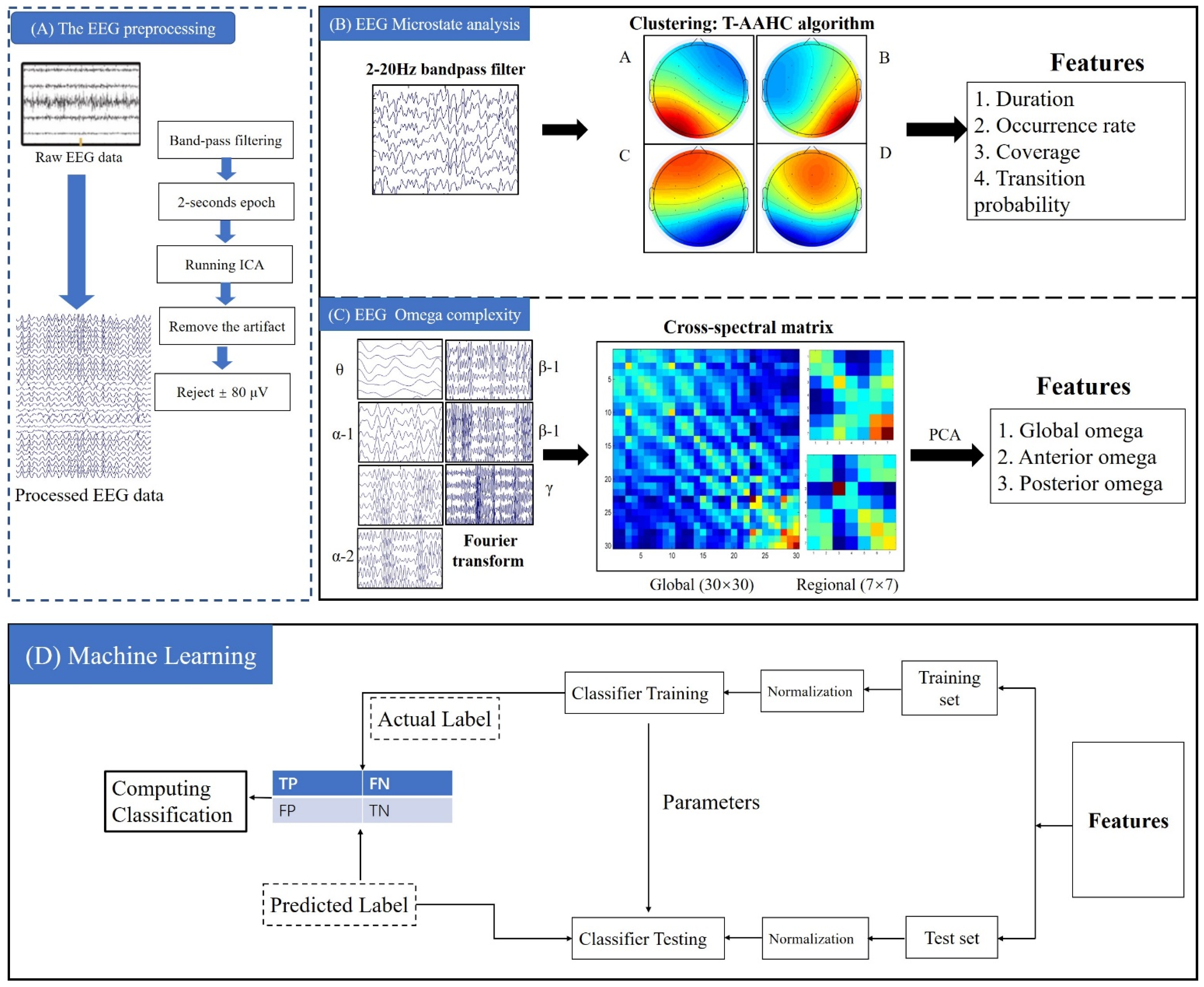
2.2. EEG Acquisition and Preprocessing
2.3. EEG Microstate Analysis
2.4. Omega Complexity Analysis
2.5. Support Vector Machine
2.6. Statistical Analysis
3. Results
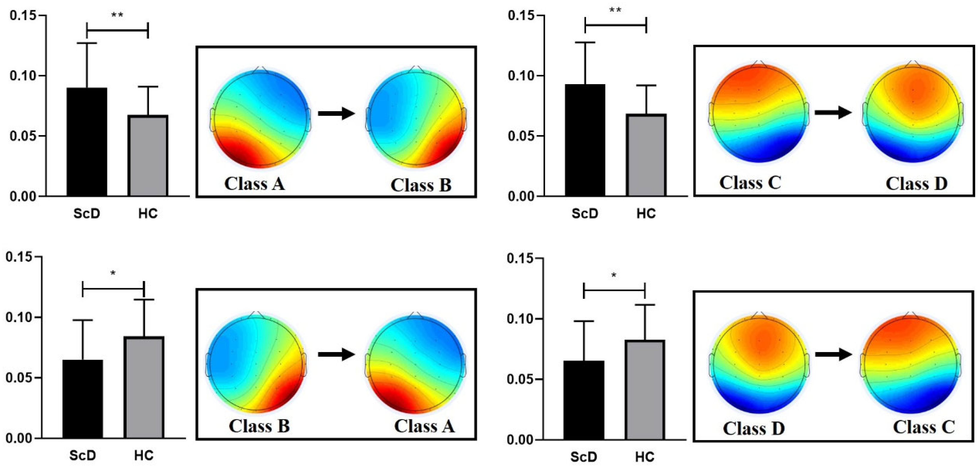
3.1. EEG Microstate
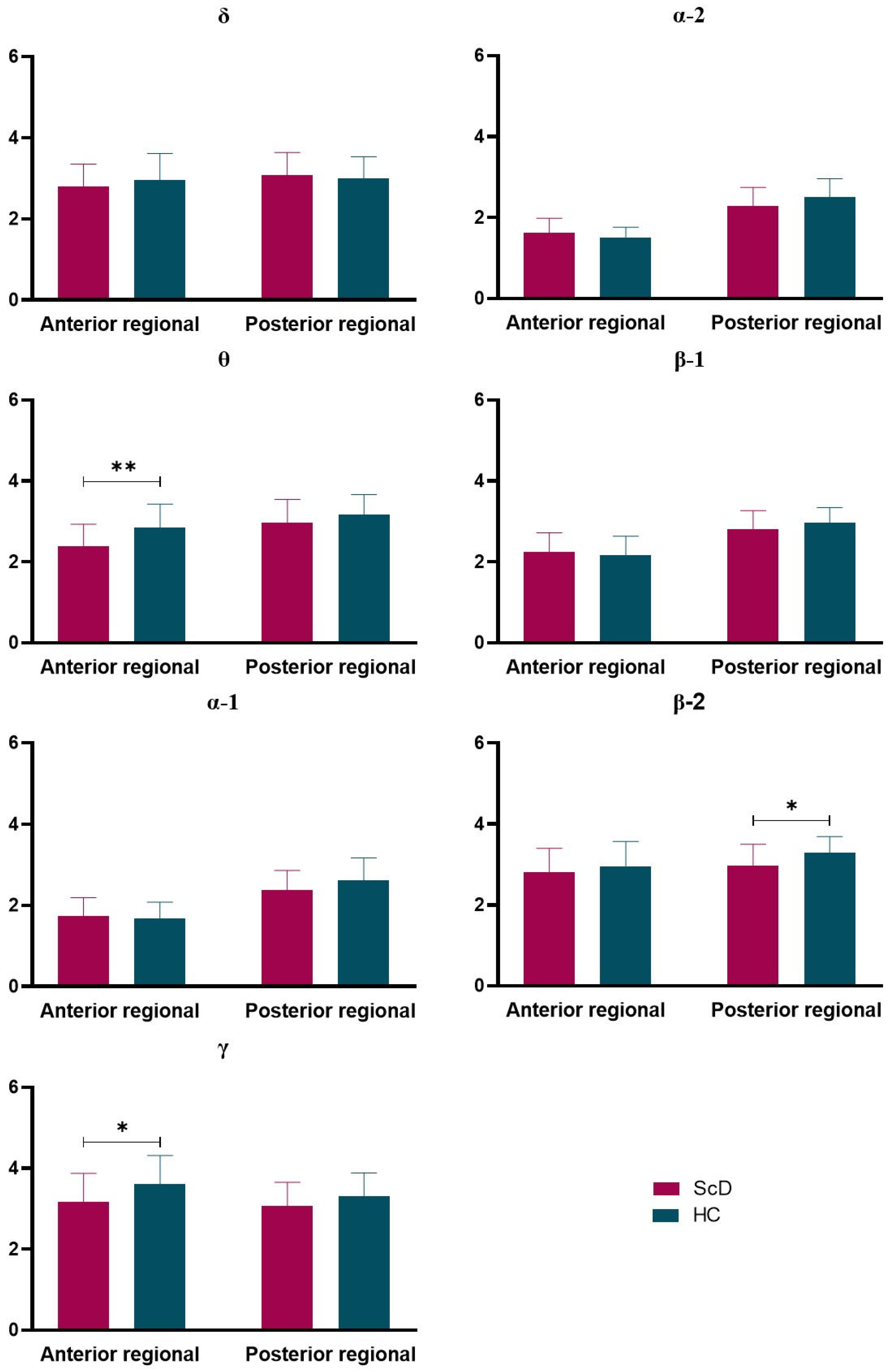
3.2. Omega Complexity
3.3. Correlations Results
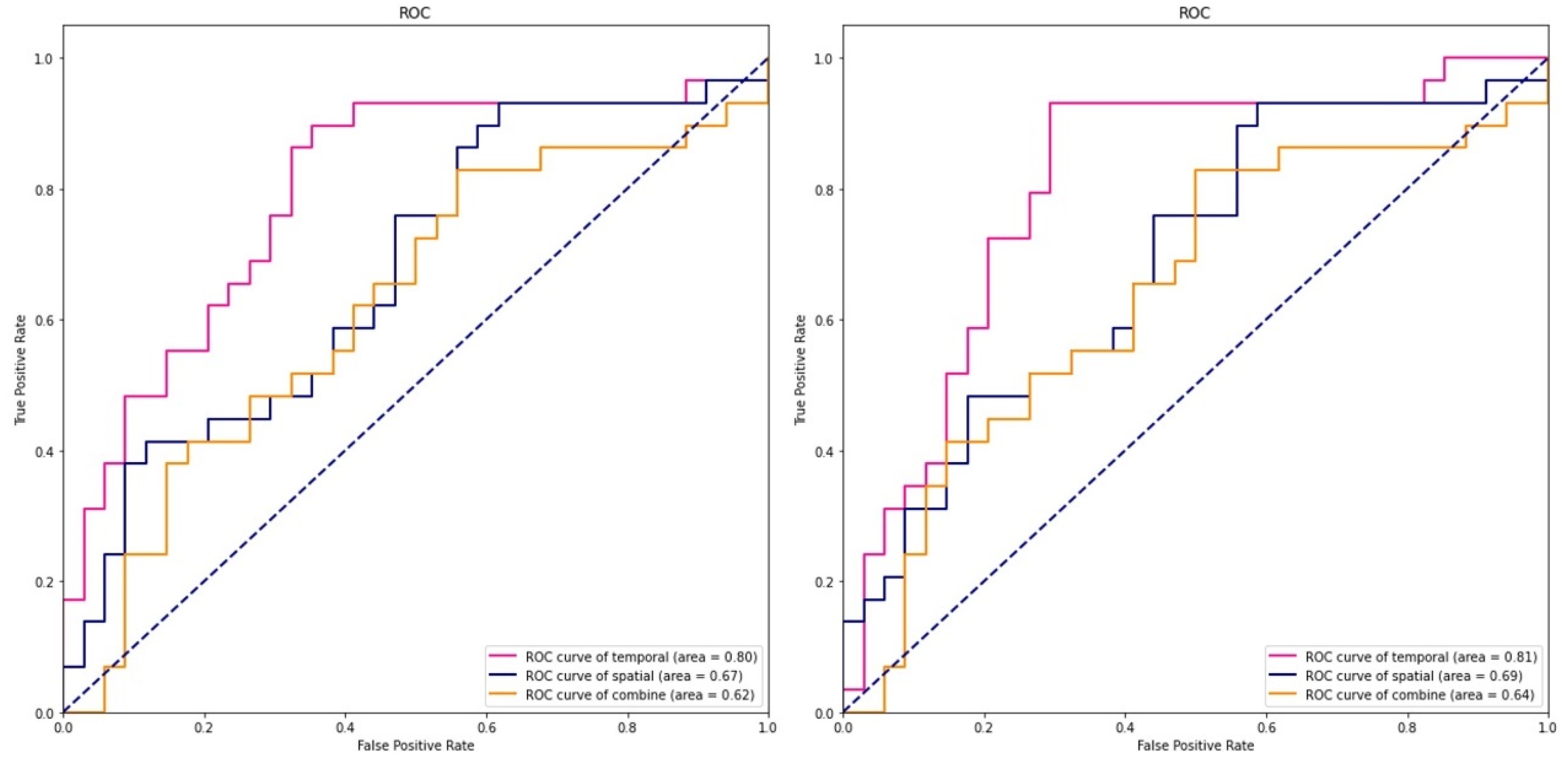
3.4. SVM Results
4. Discussion
4.1. EEG Microstates
4.2. Omega Complexity
4.3. The Classification Results
4.4. Limitations
5. Conclusions
Author Contributions
Funding
Institutional Review Board Statement
Informed Consent Statement
Data Availability Statement
Acknowledgments
Conflicts of Interest
References
- Malhi, G.S.; Mann, J.J. Depression. Lancet 2018, 392, 2299–2312. [Google Scholar] [CrossRef]
- Hamilton, J.P.; Chen, M.C.; Gotlib, I.H. Neural systems approaches to understanding major depressive disorder: An intrinsic functional organization perspective. Neurobiol. Dis. 2013, 52, 4–11. [Google Scholar] [CrossRef] [Green Version]
- Whitton, A.E.; Deccy, S.; Ironside, M.L.; Kumar, P.; Beltzer, M.; Pizzagalli, D.A. Electroencephalography Source Functional Connectivity Reveals Abnormal High-Frequency Communication Among Large-Scale Functional Networks in Depression. Biol. Psychiatry Cogn. Neurosci. Neuroimaging 2018, 3, 50–58. [Google Scholar] [CrossRef]
- Kaiser, R.H.; Andrews-Hanna, J.R.; Wager, T.D.; Pizzagalli, D.A. Large-Scale Network Dysfunction in Major Depressive Disorder: A Meta-analysis of Resting-State Functional Connectivity. JAMA Psychiatry 2015, 72, 603–611. [Google Scholar] [CrossRef]
- Pang, J.C.; Gollo, L.L.; Roberts, J.A. Stochastic synchronization of dynamics on the human connectome. Neuroimage 2021, 229, 117738. [Google Scholar] [CrossRef]
- De Pasquale, F.; Corbetta, M.; Betti, V.; Della Penna, S. Cortical cores in network dynamics. Neuroimage 2018, 180, 370–382. [Google Scholar] [CrossRef]
- De Bock, R.; Mackintosh, A.J.; Maier, F.; Borgwardt, S.; Riecher-Rössler, A.; Andreou, C. EEG microstates as biomarker for psychosis in ultra-high-risk patients. Transl. Psychiatry 2020, 10, 300. [Google Scholar] [CrossRef]
- Gao, F.; Jia, H.; Feng, Y. Microstate and Omega Complexity Analyses of the Resting-state Electroencephalography. J. Vis. Exp. 2018, e56452. [Google Scholar] [CrossRef] [Green Version]
- Li, H.; Yue, J.; Wang, Y.; Zou, F.; Zhang, M.; Wu, X. Negative Effects of Mobile Phone Addiction Tendency on Spontaneous Brain Microstates: Evidence From Resting-State EEG. Front. Hum. Neurosci. 2021, 15, 636504. [Google Scholar] [CrossRef]
- Chu, C.; Wang, X.; Cai, L.; Zhang, L.; Wang, J.; Liu, C.; Zhu, X. Spatiotemporal EEG microstate analysis in drug-free patients with Parkinson’s disease. Neuroimage Clin. 2020, 25, 102132. [Google Scholar] [CrossRef]
- Wackermann, J.; Lehmann, D.; Michel, C.M.; Strik, W.K. Adaptive segmentation of spontaneous EEG map series into spatially defined microstates. Int. J. Psychophysiol. 1993, 14, 269–283. [Google Scholar] [CrossRef]
- Andreou, C.; Faber, P.L.; Leicht, G.; Schoettle, D.; Polomac, N.; Hanganu-Opatz, I.L.; Lehmann, D.; Mulert, C. Resting-state connectivity in the prodromal phase of schizophrenia: Insights from EEG microstates. Schizophr. Res. 2014, 152, 513–520. [Google Scholar] [CrossRef]
- Dinov, M.; Leech, R. Modeling Uncertainties in EEG Microstates: Analysis of Real and Imagined Motor Movements Using Probabilistic Clustering-Driven Training of Probabilistic Neural Networks. Front. Hum. Neurosci. 2017, 11, 534. [Google Scholar] [CrossRef] [Green Version]
- Britz, J.; Diaz Hernandez, L.; Ro, T.; Michel, C.M. EEG-microstate dependent emergence of perceptual awareness. Front. Behav. Neurosci. 2014, 8, 163. [Google Scholar] [CrossRef] [PubMed] [Green Version]
- Michel, C.M.; Koenig, T. EEG microstates as a tool for studying the temporal dynamics of whole-brain neuronal networks: A review. Neuroimage 2018, 180, 577–593. [Google Scholar] [CrossRef] [PubMed]
- Khanna, A.; Pascual-Leone, A.; Michel, C.M.; Farzan, F. Microstates in resting-state EEG: Current status and future directions. Neurosci. Biobehav. Rev. 2015, 49, 105–113. [Google Scholar] [CrossRef] [PubMed] [Green Version]
- Lehmann, D.; Faber, P.L.; Galderisi, S.; Herrmann, W.M.; Kinoshita, T.; Koukkou, M.; Mucci, A.; Pascual-Marqui, R.D.; Saito, N.; Wackermann, J.; et al. EEG microstate duration and syntax in acute, medication-naive, first-episode schizophrenia: A multi-center study. Psychiatry Res. 2005, 138, 141–156. [Google Scholar] [CrossRef]
- Al Zoubi, O.; Mayeli, A.; Tsuchiyagaito, A.; Misaki, M.; Zotev, V.; Refai, H.; Paulus, M.; Bodurka, J. EEG Microstates Temporal Dynamics Differentiate Individuals with Mood and Anxiety Disorders from Healthy Subjects. Front. Hum. Neurosci. 2019, 13, 56. [Google Scholar] [CrossRef] [Green Version]
- Damborská, A.; Piguet, C.; Aubry, J.M.; Dayer, A.G.; Michel, C.M.; Berchio, C. Altered Electroencephalographic Resting-State Large-Scale Brain Network Dynamics in Euthymic Bipolar Disorder Patients. Front. Psychiatry 2019, 10, 826. [Google Scholar] [CrossRef]
- Murphy, M.; Whitton, A.E.; Deccy, S.; Ironside, M.L.; Rutherford, A.; Beltzer, M.; Sacchet, M.; Pizzagalli, D.A. Abnormalities in electroencephalographic microstates are state and trait markers of major depressive disorder. Neuropsychopharmacology 2020, 45, 2030–2037. [Google Scholar] [CrossRef]
- Strelets, V.; Faber, P.L.; Golikova, J.; Novototsky-Vlasov, V.; Koenig, T.; Gianotti, L.R.; Gruzelier, J.H.; Lehmann, D. Chronic schizophrenics with positive symptomatology have shortened EEG microstate durations. Clin. Neurophysiol. 2003, 114, 2043–2051. [Google Scholar] [CrossRef]
- Bhattacharya, J. Complexity analysis of spontaneous EEG. Acta Neurobiol. Exp. 2000, 60, 495–501. [Google Scholar]
- Catarino, A.; Churches, O.; Baron-Cohen, S.; Andrade, A.; Ring, H. Atypical EEG complexity in autism spectrum conditions: A multiscale entropy analysis. Clin. Neurophysiol. 2011, 122, 2375–2383. [Google Scholar] [CrossRef] [PubMed]
- Goldberger, A.L.; Peng, C.K.; Lipsitz, L.A. What is physiologic complexity and how does it change with aging and disease? Neurobiol. Aging 2002, 23, 23–26. [Google Scholar] [CrossRef]
- Saito, N.; Kuginuki, T.; Yagyu, T.; Kinoshita, T.; Koenig, T.; Pascual-Marqui, R.D.; Kochi, K.; Wackermann, J.; Lehmann, D. Global, regional, and local measures of complexity of multichannel electroencephalography in acute, neuroleptic-naive, first-break schizophrenics. Biol. Psychiatry 1998, 43, 794–802. [Google Scholar] [CrossRef]
- Kikuchi, M.; Hashimoto, T.; Nagasawa, T.; Hirosawa, T.; Minabe, Y.; Yoshimura, M.; Strik, W.; Dierks, T.; Koenig, T. Frontal areas contribute to reduced global coordination of resting-state gamma activities in drug-naïve patients with schizophrenia. Schizophr. Res. 2011, 130, 187–194. [Google Scholar] [CrossRef]
- Gao, F.; Jia, H.; Wu, X.; Yu, D.; Feng, Y. Altered Resting-State EEG Microstate Parameters and Enhanced Spatial Complexity in Male Adolescent Patients with Mild Spastic Diplegia. Brain Topogr. 2017, 30, 233–244. [Google Scholar] [CrossRef] [PubMed]
- Satterthwaite, T.D.; Kable, J.W.; Vandekar, L.; Katchmar, N.; Bassett, D.S.; Baldassano, C.F.; Ruparel, K.; Elliott, M.A.; Sheline, Y.I.; Gur, R.C.; et al. Common and Dissociable Dysfunction of the Reward System in Bipolar and Unipolar Depression. Neuropsychopharmacology 2015, 40, 2258–2268. [Google Scholar] [CrossRef] [Green Version]
- Wu, X.; Lin, P.; Yang, J.; Song, H.; Yang, R.; Yang, J. Dysfunction of the cingulo-opercular network in first-episode medication-naive patients with major depressive disorder. J. Affect. Disord. 2016, 200, 275–283. [Google Scholar] [CrossRef]
- Karsten, J.; Hartman, C.A.; Smit, J.H.; Zitman, F.G.; Beekman, A.T.; Cuijpers, P.; van der Does, A.J.; Ormel, J.; Nolen, W.A.; Penninx, B.W. Psychiatric history and subthreshold symptoms as predictors of the occurrence of depressive or anxiety disorder within 2 years. Br. J. Psychiatry 2011, 198, 206–212. [Google Scholar] [CrossRef]
- Murphy, J.M.; Nierenberg, A.A.; Laird, N.M.; Monson, R.R.; Sobol, A.M.; Leighton, A.H. Incidence of major depression: Prediction from subthreshold categories in the Stirling County Study. J. Affect. Disord. 2002, 68, 251–259. [Google Scholar] [CrossRef]
- Guo, L.; Cao, J.; Cheng, P.; Shi, D.; Cao, B.; Yang, G.; Liang, S.; Su, N.; Yu, M.; Zhang, C.; et al. Moderate-to-Severe Depression Adversely Affects Lung Function in Chinese College Students. Front. Psychol. 2020, 11, 652. [Google Scholar] [CrossRef] [PubMed] [Green Version]
- Chai, L.; Yang, W.; Zhang, J.; Chen, S.; Hennessy, D.A.; Liu, Y. Relationship between Perfectionism and Depression among Chinese College Students with Self-Esteem as a Mediator. Omega 2020, 80, 490–503. [Google Scholar] [CrossRef] [PubMed]
- Fountoulakis, K.N.; Apostolidou, M.K.; Atsiova, M.B.; Filippidou, A.K.; Florou, A.K.; Gousiou, D.S.; Katsara, A.R.; Mantzari, S.N.; Padouva-Markoulaki, M.; Papatriantafyllou, E.I.; et al. Self-reported changes in anxiety, depression and suicidality during the COVID-19 lockdown in Greece. J. Affect. Disord. 2021, 279, 624–629. [Google Scholar] [CrossRef] [PubMed]
- Cuijpers, P.; Smit, F. Subclinical depression: A clinically relevant condition? Tijdschr. Psychiatr. 2008, 50, 519–528. [Google Scholar]
- Parker, G.; Brotchie, H. Gender differences in depression. Int. Rev. Psychiatry 2010, 22, 429–436. [Google Scholar] [CrossRef]
- Van de Velde, S.; Bracke, P.; Levecque, K. Gender differences in depression in 23 European countries. Cross-national variation in the gender gap in depression. Soc. Sci. Med. 2010, 71, 305–313. [Google Scholar] [CrossRef]
- Cabitza, F.; Banfi, G. Machine learning in laboratory medicine: Waiting for the flood? Clin. Chem. Lab. Med. 2018, 56, 516–524. [Google Scholar] [CrossRef]
- Senders, J.T.; Staples, P.C.; Karhade, A.V.; Zaki, M.M.; Gormley, W.B.; Broekman, M.L.D.; Smith, T.R.; Arnaout, O. Machine Learning and Neurosurgical Outcome Prediction: A Systematic Review. World Neurosurg. 2018, 109, 476–486. [Google Scholar] [CrossRef]
- Shin, D.; Lee, K.J.; Adeluwa, T.; Hur, J. Machine Learning-Based Predictive Modeling of Postpartum Depression. J. Clin. Med. 2020, 9, 2899. [Google Scholar] [CrossRef]
- Shatte, A.B.R.; Hutchinson, D.M.; Teague, S.J. Machine learning in mental health: A scoping review of methods and applications. Psychol. Med. 2019, 49, 1426–1448. [Google Scholar] [CrossRef] [PubMed] [Green Version]
- Zhao, K.; So, H.C. Drug Repositioning for Schizophrenia and Depression/Anxiety Disorders: A Machine Learning Approach Leveraging Expression Data. IEEE J. Biomed. Health Inform. 2019, 23, 1304–1315. [Google Scholar] [CrossRef] [PubMed]
- Lee, Y.; Ragguett, R.M.; Mansur, R.B.; Boutilier, J.J.; Rosenblat, J.D.; Trevizol, A.; Brietzke, E.; Lin, K.; Pan, Z.; Subramaniapillai, M.; et al. Applications of machine learning algorithms to predict therapeutic outcomes in depression: A meta-analysis and systematic review. J. Affect. Disord. 2018, 241, 519–532. [Google Scholar] [CrossRef] [PubMed]
- Mao, N.; Che, K.; Chu, T.; Li, Y.; Wang, Q.; Liu, M.; Ma, H.; Wang, Z.; Lin, F.; Wang, B.; et al. Aberrant Resting-State Brain Function in Adolescent Depression. Front. Psychol. 2020, 11, 1784. [Google Scholar] [CrossRef]
- Zung, W.W. A self-rating depression scale. Arch. Gen. Psychiatry 1965, 12, 63–70. [Google Scholar] [CrossRef]
- Wang, Y.P.; Gorenstein, C. Psychometric properties of the Beck Depression Inventory-II: A comprehensive review. Braz. J. Psychiatry 2013, 35, 416–431. [Google Scholar] [CrossRef] [Green Version]
- Wang, Z.; Yuan, C.M.; Huang, J.; Li, Z.Z.; Chen, J.; Zhang, H.Y.; Fang, Y.R.; Xiao, Z.P. Reliability and validity of the Chinese version of Beck Depression Inventory-H among depression patients. Chin. Ment. Health J. 2011, 25, 476–480. [Google Scholar]
- Yang, T.; Xiang, L. Executive control dysfunction in subclinical depressive undergraduates: Evidence from the Attention Network Test. J. Affect. Disord. 2019, 245, 130–139. [Google Scholar] [CrossRef]
- Oldfield, R.C. The assessment and analysis of handedness: The Edinburgh inventory. Neuropsychologia 1971, 9, 97–113. [Google Scholar] [CrossRef]
- Schlegel, F.; Lehmann, D.; Faber, P.L.; Milz, P.; Gianotti, L.R. EEG microstates during resting represent personality differences. Brain Topogr. 2012, 25, 20–26. [Google Scholar] [CrossRef] [Green Version]
- Faul, F.; Erdfelder, E.; Buchner, A.; Lang, A.G. Statistical power analyses using G*Power 3.1: Tests for correlation and regression analyses. Behav. Res. Methods 2009, 41, 1149–1160. [Google Scholar] [CrossRef] [Green Version]
- Kikuchi, M.; Koenig, T.; Munesue, T.; Hanaoka, A.; Strik, W.; Dierks, T.; Koshino, Y.; Minabe, Y. EEG microstate analysis in drug-naive patients with panic disorder. PLoS ONE 2011, 6, e22912. [Google Scholar] [CrossRef] [Green Version]
- Rieger, K.; Diaz Hernandez, L.; Baenninger, A.; Koenig, T. 15 Years of Microstate Research in Schizophrenia—Where Are We? A Meta-Analysis. Front. Psychiatry 2016, 7, 22. [Google Scholar] [CrossRef] [Green Version]
- Ahmadi, N.; Pei, Y.; Carrette, E.; Aldenkamp, A.P.; Pechenizkiy, M. EEG-based classification of epilepsy and PNES: EEG microstate and functional brain network features. Brain Inform. 2020, 7, 6. [Google Scholar] [CrossRef]
- Xu, J.; Pan, Y.; Zhou, S.; Zou, G.; Liu, J.; Su, Z.; Zou, Q.; Gao, J.H. EEG microstates are correlated with brain functional networks during slow-wave sleep. Neuroimage 2020, 215, 116786. [Google Scholar] [CrossRef] [PubMed]
- Musaeus, C.S.; Nielsen, M.S.; Høgh, P. Microstates as Disease and Progression Markers in Patients With Mild Cognitive Impairment. Front. Neurosci. 2019, 13, 563. [Google Scholar] [CrossRef] [PubMed] [Green Version]
- Milz, P.; Faber, P.L.; Lehmann, D.; Koenig, T.; Kochi, K.; Pascual-Marqui, R.D. The functional significance of EEG microstates—Associations with modalities of thinking. Neuroimage 2016, 125, 643–656. [Google Scholar] [CrossRef]
- Milz, P.; Pascual-Marqui, R.D.; Achermann, P.; Kochi, K.; Faber, P.L. The EEG microstate topography is predominantly determined by intracortical sources in the alpha band. Neuroimage 2017, 162, 353–361. [Google Scholar] [CrossRef] [PubMed] [Green Version]
- Dedovic, K.; Renwick, R.; Mahani, N.K.; Engert, V.; Lupien, S.J.; Pruessner, J.C. The Montreal Imaging Stress Task: Using functional imaging to investigate the effects of perceiving and processing psychosocial stress in the human brain. J. Psychiatry Neurosci. 2005, 30, 319–325. [Google Scholar] [PubMed]
- Taylor, K.S.; Seminowicz, D.A.; Davis, K.D. Two systems of resting state connectivity between the insula and cingulate cortex. Hum. Brain Mapp. 2009, 30, 2731–2745. [Google Scholar] [CrossRef]
- Pollatos, O.; Gramann, K.; Schandry, R. Neural systems connecting interoceptive awareness and feelings. Hum. Brain Mapp. 2007, 28, 9–18. [Google Scholar] [CrossRef] [PubMed]
- Müller, T.J.; Koenig, T.; Wackermann, J.; Kalus, P.; Fallgatter, A.; Strik, W.; Lehmann, D. Subsecond changes of global brain state in illusory multistable motion perception. J. Neural Transm. 2005, 112, 565–576. [Google Scholar] [CrossRef] [PubMed]
- Murphy, M.; Stickgold, R.; Öngür, D. Electroencephalogram Microstate Abnormalities in Early-Course Psychosis. Biol. Psychiatry Cogn. Neurosci. Neuroimaging 2020, 5, 35–44. [Google Scholar] [CrossRef] [PubMed]
- Dimitriadis, S.I.; Sun, Y.; Kwok, K.; Laskaris, N.A.; Thakor, N.; Bezerianos, A. Cognitive workload assessment based on the tensorial treatment of EEG estimates of cross-frequency phase interactions. Ann. Biomed. Eng. 2015, 43, 977–989. [Google Scholar] [CrossRef]
- Li, Y.; Kang, C.; Qu, X.; Zhou, Y.; Wang, W.; Hu, Y. Depression-Related Brain Connectivity Analyzed by EEG Event-Related Phase Synchrony Measure. Front. Hum. Neurosci. 2016, 10, 477. [Google Scholar] [CrossRef] [PubMed] [Green Version]
- Li, Y.; Cao, D.; Wei, L.; Tang, Y.; Wang, J. Abnormal functional connectivity of EEG gamma band in patients with depression during emotional face processing. Clin. Neurophysiol. 2015, 126, 2078–2089. [Google Scholar] [CrossRef] [PubMed]
- Sun, J.; Wang, B.; Niu, Y.; Tan, Y.; Fan, C.; Zhang, N.; Xue, J.; Wei, J.; Xiang, J. Complexity Analysis of EEG, MEG, and fMRI in Mild Cognitive Impairment and Alzheimer’s Disease: A Review. Entropy 2020, 22, 239. [Google Scholar] [CrossRef] [Green Version]
- Mumtaz, W.; Ali, S.S.A.; Yasin, M.A.M.; Malik, A.S. A machine learning framework involving EEG-based functional connectivity to diagnose major depressive disorder (MDD). Med. Biol. Eng. Comput. 2018, 56, 233–246. [Google Scholar] [CrossRef]
- Mumtaz, W.; Xia, L.; Mohd Yasin, M.A.; Azhar Ali, S.S.; Malik, A.S. A wavelet-based technique to predict treatment outcome for Major Depressive Disorder. PLoS ONE 2017, 12, e0171409. [Google Scholar] [CrossRef] [Green Version]


| Variable | HCs (n = 38) | ScD (n = 40) |
|---|---|---|
| Age, years | 18.72 ± 0.36 | 18.51 ± 0.42 |
| Height, cm | 162.71± 6.62 | 160.70 ± 6.73 |
| Weight, kg | 52.37 ± 4.72 | 50.00 ± 1.92 |
| BMI, kg/m2 | 20.79 ± 2.73 | 19.43 ±1.61 |
| SDS | 10.57 ± 5.47 | 66.71 ± 5.38 *** |
| BDI-II | 3.46 ± 0.73 | 24.86 ± 2.02 *** |
| Class A | Class B | Class C | Class D | |||||
|---|---|---|---|---|---|---|---|---|
| Mean | SD | Mean | SD | Mean | SD | Mean | SD | |
| Duration (ms) | ||||||||
| ScD group | 71.50 | 12.13 | 64.53 | 8.99 | 62.91 | 12.52 | 67.77 | 34.68 |
| HCs group | 73.32 | 14.36 | 66.92 | 12.06 | 73.77 | 17.49 | 64.85 | 16.09 |
| t (df = 61) | −0.546 | −0.899 | −2.891 | 0.415 | ||||
| p | 0.308 | 0.206 | 0.005 | 0.679 | ||||
| Cohen’s d | 0.14 | 0.22 | 0.74 | 0.11 | ||||
| Occurrence/s | ||||||||
| ScD group | 4.06 | 0.80 | 3.81 | 0.93 | 3.62 | 1.02 | 3.34 | 1.26 |
| HCs group | 3.67 | 0.83 | 3.27 | 0.98 | 4.03 | 0.74 | 3.28 | 0.92 |
| t (df = 61) | 1.882 | 2.256 | −1.784 | 0.221 | ||||
| p | 0.065 | 0.028 | 0.078 | 0.826 | ||||
| Cohen’s d | 0.52 | 0.56 | 0.46 | 0.05 | ||||
| Contribution (%) | ||||||||
| ScD group | 28.98 | 8.79 | 24.62 | 7.54 | 23.14 | 9.12 | 23.25 | 14.06 |
| HCs group | 26.90 | 9.17 | 21.96 | 8.97 | 29.26 | 8.34 | 21.88 | 9.75 |
| t (df = 61) | 0.917 | 1.283 | −2.758 | 0.442 | ||||
| p | 0.363 | 0.204 | 0.008 | 0.660 | ||||
| Cohen’s d | 0.23 | 0.32 | 0.70 | 0.11 | ||||
| ScD | HCs | t (df = 61) | p | Cohen’s d | |
|---|---|---|---|---|---|
| Delta | 4.75 ± 1.03 | 4.72 ± 1.02 | 0.118 | 0.906 | 0.03 |
| Theta | 4.27 ± 0.89 | 4.64 ± 0.97 | −1.582 | 0.119 | 0.41 |
| Alpha1 | 2.86 ± 0.67 | 2.95 ± 0.92 | −0.464 | 0.644 | 0.12 |
| Alpha2 | 2.72 ± 0.57 | 2.73 ± 0.63 | −0.044 | 0.965 | 0.01 |
| Beta1 | 3.92 ± 0.71 | 3.91 ± 0.70 | 0.069 | 0.945 | 0.02 |
| Beta2 | 4.63 ± 0.92 | 5.21 ± 0.93 | −2.452 | 0.017 | 0.63 |
| Gamma | 5.38 ± 1.34 | 6.21 ± 1.24 | −2.546 | 0.013 | 0.65 |
| EEG Features | Linear Kernel Function | Gaussian Kernel Function | ||
|---|---|---|---|---|
| Accuracy | AUC | Accuracy | AUC | |
| Microstate | 62% | 67% | 63% | 69% |
| Omega complexity | 60% | 62% | 60% | 64% |
| Combine | 75% | 80% | 76% | 81% |
Publisher’s Note: MDPI stays neutral with regard to jurisdictional claims in published maps and institutional affiliations. |
© 2022 by the authors. Licensee MDPI, Basel, Switzerland. This article is an open access article distributed under the terms and conditions of the Creative Commons Attribution (CC BY) license (https://creativecommons.org/licenses/by/4.0/).
Share and Cite
Zhao, S.; Ng, S.-C.; Khoo, S.; Chi, A. Temporal and Spatial Dynamics of EEG Features in Female College Students with Subclinical Depression. Int. J. Environ. Res. Public Health 2022, 19, 1778. https://doi.org/10.3390/ijerph19031778
Zhao S, Ng S-C, Khoo S, Chi A. Temporal and Spatial Dynamics of EEG Features in Female College Students with Subclinical Depression. International Journal of Environmental Research and Public Health. 2022; 19(3):1778. https://doi.org/10.3390/ijerph19031778
Chicago/Turabian StyleZhao, Shanguang, Siew-Cheok Ng, Selina Khoo, and Aiping Chi. 2022. "Temporal and Spatial Dynamics of EEG Features in Female College Students with Subclinical Depression" International Journal of Environmental Research and Public Health 19, no. 3: 1778. https://doi.org/10.3390/ijerph19031778
APA StyleZhao, S., Ng, S.-C., Khoo, S., & Chi, A. (2022). Temporal and Spatial Dynamics of EEG Features in Female College Students with Subclinical Depression. International Journal of Environmental Research and Public Health, 19(3), 1778. https://doi.org/10.3390/ijerph19031778