


Sensitivity of a Dynamic Model of Air Traffic Emissions to Technological and Environmental Factors

 , and
, and
Abstract
1. Introduction
2. Models of the CO Emissions Generated by Air Traffic
3. Data and Methodology
3.1. Data
3.2. Methodology
3.2.1. Morris Sensitivity Analysis
3.2.2. Sobol Sensitivity Analysis
4. Results and Discussion
4.1. Model Configuration
4.2. Characterization of the Model Complexity
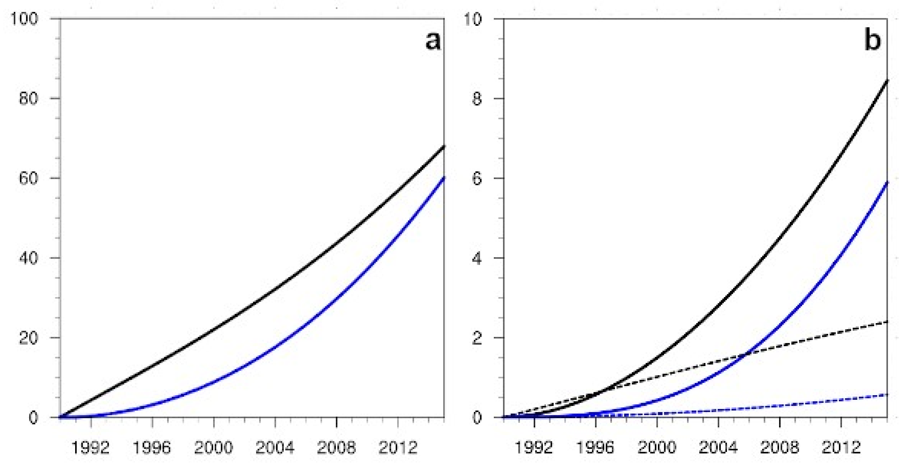
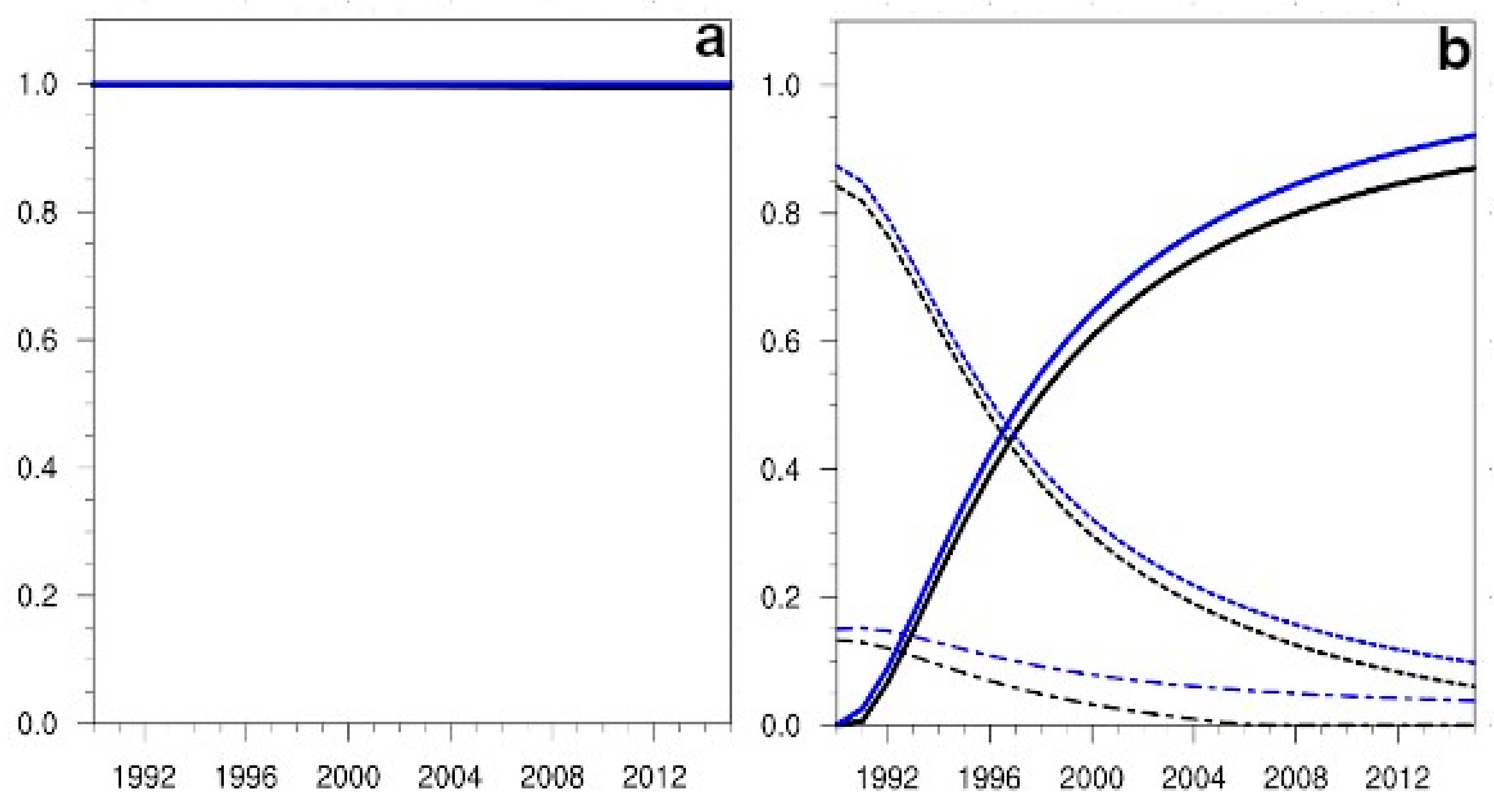
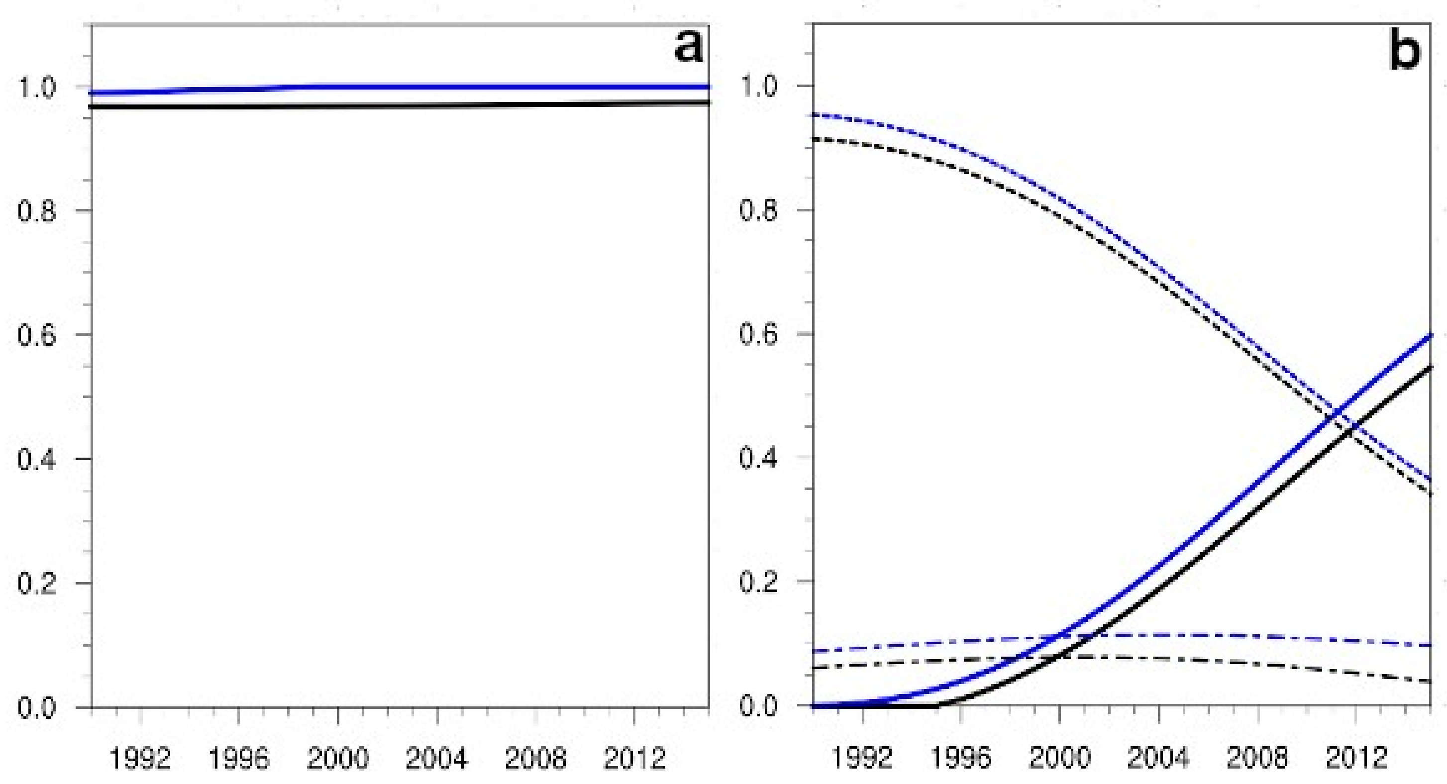
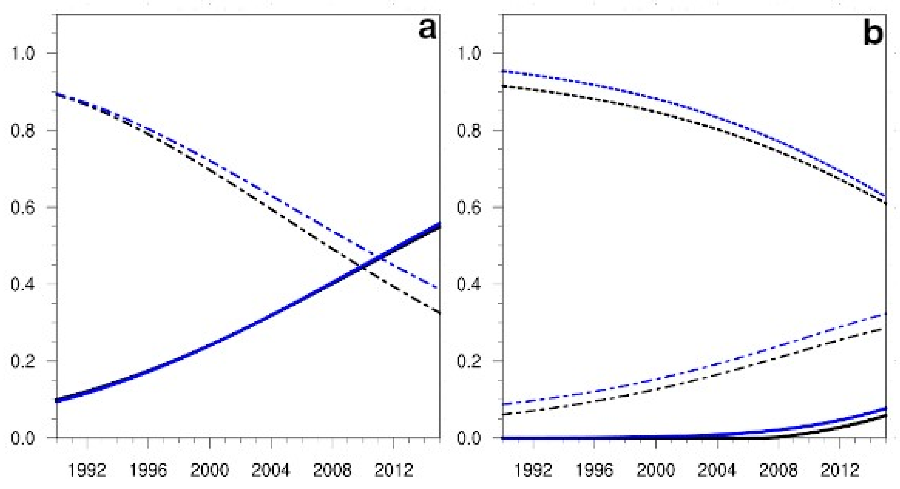
4.3. Results of the Global Sensitivity Analysis
4.3.1. The GSA for a Wide Range of Non-Linear Parameter Values
4.3.2. A Case Study: The GSA for Small Values of the Nonlinear Parameter
5. Summary
6. Conclusions
Supplementary Materials
Author Contributions
Funding
Institutional Review Board Statement
Informed Consent Statement
Data Availability Statement
Acknowledgments
Conflicts of Interest
Appendix A. The Non-Linear Model
References
- Morris, M.D. Factorial sampling plans for preliminary computational experiments. Technometrics 1991, 33, 161–174. Available online: http://www.jstor.org/stable/1269043 (accessed on 14 May 2022). [CrossRef]
- Sobol, I.M. Global sensitivity indices for nonlinear mathematical models and their Monte Carlo estimates. Math. A Comput. Sim. 2001, 55, 271–280. [Google Scholar] [CrossRef]
- Homma, T.; Saltelli, A. Importance measures in global sensitivity analysis of nonlinear models. Reliab. Eng. Syst. Saf. 1996, 52, 1–17. [Google Scholar] [CrossRef]
- Liu, Q.; Homma, T. A new computational method of a moment-independent uncertainty importance measure. Reliab. Eng. Syst. Saf. 2009, 94, 1205–1211. [Google Scholar] [CrossRef]
- Cariboni, J.; Campolongo, F. Grouping model input factors to perform a sensitivity analysis computationally efficient. In Probabilistic Safety Assessment and Management; Spitzer, C., Schmocker, U., Dang, V.N., Eds.; Springer: London, UK, 2004; pp. 2018–2023. [Google Scholar] [CrossRef]
- Campolongo, F.; Saltelli, A.; Cariboni, J. From screening to quantitative sensitivity analysis. A unified approach. Comp. Phys. Commun. 2011, 182, 978–988. [Google Scholar] [CrossRef]
- Sobol, I.M.; Kucherenko, S. Derivative based global sensitivity measures and their link with global sensitivity indices. Math. A Comput. Sim. 2009, 79, 3009–3017. [Google Scholar] [CrossRef]
- Tang, Z.; Zuo, M.J.; Xiao, N. An efficient method for evaluating the effect of input parameters on the integrity of safety systems. Reliab. Eng. Syst. Saf. 2016, 145, 111–123. [Google Scholar] [CrossRef]
- Tang, Z.; Zuo, M.J.; Xia, Y. Effect of truncated input parameter distribution on the integrity of safety instrumented systems under epistemic uncertainty. IEEE Trans. Reliab. 2017, 66, 735–750. [Google Scholar] [CrossRef]
- Schmolke, A.; Thorbek, P.; DeAngelis, D.L.; Grimm, V. Ecological models supporting environmental decision making: A strategy for the future. Trends Ecol. Evol. 2010, 25, 479–486. [Google Scholar] [CrossRef] [PubMed]
- Lamboni, M.; Monod, H.; Makowski, D. Multivariate sensitivity analysis to measure global contribution of input factors in dynamic models. Reliab. Eng. Syst. Saf. 2011, 96, 450–459. [Google Scholar] [CrossRef]
- Sarrazin, F.; Pianosi, F.; Wagener, T. Global sensitivity analysis of environmental models: Convergence and validation. Environ. Model. Soft. 2016, 79, 135–152. [Google Scholar] [CrossRef]
- Kent, E.; Neumann, S.; Kummer, U.; Mendes, P. What Can We Learn from Global Sensitivity Analysis of Biochemical Systems? PLoS ONE 2013, 8, e79244. [Google Scholar] [CrossRef] [PubMed]
- Almeida, S.; Holcombre, E.A.; Pianosi, F.; Wagener, T. Dealing with deep uncertainties in landslide modelling for disaster risk reduction under climate change. Nat. Haz. Earth. Sys. Sci. 2017, 17, 225–241. [Google Scholar] [CrossRef]
- Garcia, D.; Arostegui, I.; Prellezo, R. Robust combination of the Morris and Sobol methods in complex multidimensional models. Environ. Model. Soft. 2019, 122, 104517. [Google Scholar] [CrossRef]
- Buendia-Hernandez, F.A.; Alvarez-Garcia, F.J.; OrtizBevia, M.J.; RuizdeElvira, A. Dynamic modelling of traffic emissions with a two variables system. Int. J. Sustain. Transport. 2021, 16, 1–10. [Google Scholar] [CrossRef]
- Shepherd, D.; Dirks, K.; Welch, D.; McBride, D.; Landon, J. The Covariance between Air Pollution Annoyance and Noise Annoyance, and Its Relationship with Health-Related Quality of Life. Int. J. Environ. Res. Public Health 2016, 13, 792. [Google Scholar] [CrossRef]
- Grewe, V.; Gangoli Rao, A.; Grönstedt, T.; Xisto, C.; Linke, F.; Melkert, J.; Middel, J.; Ohlenforst, B.; Blakey, S.; Christie, C.; et al. Evaluating the climate impact of aviation emission scenarios towards the Paris Agreement including COVID-19 effects. Nat. Commun. 2021, 12, 1–10. [Google Scholar] [CrossRef] [PubMed]
- IPCC. Intergovernmental Climate Change Panel 1995. First Approach of CO2 Equivalent. Available online: https://www.ipcc.ch/site/assets/uploads/2018/02/ipcc_wg3_ar5_annex-ii.pdf (accessed on 16 May 2022).
- IPCC. Intergovernmental Climate Change Panel 2000: Data Updated with the CO2 Equivalent. Available online: https://www.ipcc.ch/site/assets/uploads/2018/03/emissions_scenarios-1.pdf (accessed on 16 May 2022).
- Jungblut, N.; Meili, C. Aviation and Climate Change: Best Practice for Calculation of the Global Warming Potential; EsSU-Services Ltd.: Singapore, 2018. [Google Scholar] [CrossRef]
- Chèze, B.; Gastineau, P.; Chevallier, J. Forecasting world and regional aviation jet fuel demands to the mid-term 2025. Energy Policy 2011, 39, 5147–5158. [Google Scholar] [CrossRef]
- Chèze, B.; Gastineau, P.; Chevallier, J. Will technological progress be suficient to stabilize CO2 emissions from air transport at mid-term? Transport. Res. Part D 2013, 18, 91–96. [Google Scholar] [CrossRef]
- Chen, D.; Hu, M.; Han, K.; Zhang, H.; Yin, J. Short-medium-term prediction for the aviation emissions in the en route airspace considering the fluctuation of air traffic demand. Transport. Res. Part D 2016, 48, 46–62. [Google Scholar] [CrossRef]
- Andrejiova, M.; Grincova, A.; Marasova, D. Study of the Percentage of Greenhouse Gas Emissions from Aviation in the EU-27 Countries by Applying Multiple-Criteria Statistical Methods. Int. J. Environ. Res. Public Health 2020, 17, 3759. [Google Scholar] [CrossRef]
- Randers, J. 2052: A Global Forecast for the Next Forty Years; Chelsea Green Publishing: Hartford, VT, USA, 2012. [Google Scholar]
- European Commission. Flight Path 2050. Europe’s Vision for Aviation: Maintaining Global Leadership and Serving the Society Needs; Publication Office: Singapore, 2012. [Google Scholar] [CrossRef]
- European Commission. 2 Million Ton Per Year: A Performing Biofuels Supply Chain for EU Aviation; Maniatos, K., Weitz, M., Zschocke, A., Eds.; European Commission: Brussels, Belgium, 2012. Available online: http://www.unece.lsu.edu/ebusiness/documents/2013Mar/sc13_09.pdf (accessed on 11 April 2022).
- Lenzen, M.; Li, M.; Malik, A.; Pomponi, F.; Sun, Y.Y.; Wiedmann, T.; Faturay, F.; Fry, J.; Gallego, B.; Geschke, A.; et al. Global socio-economic losses and environmental gains from the Coronavirus pandemic. PLoS ONE 2020, 15, e0235654. [Google Scholar] [CrossRef]
- ICAO. Environmental Report. 2016. Available online: https://www.icao.int/environmental-protection/Pages/env2016.asp (accessed on 11 April 2022).
- LIPASTO. VTT Technical Research Centre of Finland: Espoo, Finland. 2008. Available online: http://lipasto.vtt.fi/yksikkopaastot/henkiloliikennee/ilmaliikennee/ilmae.htm (accessed on 16 February 2022).
- IPCC. Climate Change 2007: Mitigation. Contribution of Working Group III to the Fourth Assessment Report of the Intergovernmental Panel on Climate Change; Cambridge University Press: Cambridge, UK, 2007; Available online: https://www.ipcc.ch/site/assets/uploads/2018/03/ar4_wg2_full_report.pdf (accessed on 16 February 2022).
- IPCC. Climate Change 2014: Mitigation of Climate Change. Contribution of Working Group III to the Fifth Assessment Report of the Intergovernmental Panel on Climate Change; Cambridge University Press: Cambridge, UK, 2014. [Google Scholar] [CrossRef]
- Pejovic, T.; Noland, R.B.; Williams, V.; Toumi, R. Estimates of UK CO2 emissions from aviation using air traffic data. Clim. Chang. 2008, 8, 367–384. [Google Scholar] [CrossRef]
- Peeters, P.; William, V. Calculating emissions and radiative forcing: Global, national, local, individual. In Climate Change and Aviation: Issues, Challenges and Solutions; Gossling, S., Upham, P., Eds.; Earthscan Pub.: London, UK, 2009. [Google Scholar]
- Owen, B.; Lee, D.S.; Lim, L. Flying into the future: Aviation emissions scenarios to 2050. Environ. Sci. Technol. 2010, 40, 2255–2260. [Google Scholar] [CrossRef] [PubMed]
- Wasiuk, D.K.; Lowenberg, M.H.; Shallcross, D.E. An aircraft performance model implementation for the estimation of global and regional commercial aviation fuel burn and emissions. Transport. Res. Part D 2015, 35, 142–159. [Google Scholar] [CrossRef]
- Scheelhaase, J.D.; Dahlmann, K.; Jung, M.; Keimel, H.; Wolters, F. How to best address aviations full climate impact from an economic policy point of view—Main results from AviClim research project. Transport. Res. Part D 2014, 45, 112–125. [Google Scholar] [CrossRef]
- Van Manen, J.; Grewe, V. Algorithmic climate change functions for the use in eco-efficient flight planning. Transport. Res. Part D 2019, 67, 388–405. [Google Scholar] [CrossRef]
- Lee, D.S.; Fahey, D.V.; Forster, P.M.; Newton, P.J.; Wit, R.C.N.; Lim, L.L.; Owen, B.; Sausen, R. Aviation and global climate change in the 21st century. Atmos. Environ. 2009, 43, 3520–3537. [Google Scholar] [CrossRef] [PubMed]
- Lee, J.S.; Mo, J.H. Analysis of technological innovation and environmental performance improvement in the aviation sector. Int. J. Environ. Res. Public Health 2011, 8, 3777–3795. [Google Scholar] [CrossRef]
- Kreuz, M.; Nokkala, M. Extreme Weather events and the European aviation industry. In WCTR2013RIO Selected Proceedings; VTT Technical Research Center: Espoo, Finland, 2013; Available online: https://cris.vtt.fi/en/publications/extreme-weather-events-and-the-european-aviation-industry-? (accessed on 16 February 2022).
- Chen, Z.; Wang, Y. Impacts of severe weather events on high-speed rail and aviation delays. Transport. Res. Part D 2019, 69, 168–183. [Google Scholar] [CrossRef]
- Davison, L.; Littleford, C.; Ryley, T. Air travel attitudes and behaviors: The development of environmental based segments. J. Air Transp. Manag. 2014, 36, 13–22. [Google Scholar] [CrossRef]
- Fletcher, J.; Higham, J.; Longnecker, N. Climate change risk perception in the USA and alignment within sustainable travel behaviours. PLoS ONE 2021, 16, e0244545. [Google Scholar] [CrossRef]
- Lu, J.-L.; Wang, C.-Y. Investigating the impacts of air travellers’ environmental knowledge on attitudes toward carbon offsetting and willingness to mitigate the environmental impacts of aviation. Transport. Res. Part D 2018, 59, 96–107. [Google Scholar] [CrossRef]
- Choi, A.S.; Gösling, S.; Ritchie, B.W. Flying with climate liability? Transport. Res. Part D 2018, 62, 225–235. [Google Scholar] [CrossRef]
- Deutsche Luft und Raumfahrt (DLR). Analyses of the European Air Transport Market; Annual Report 2008; Release 2.1; Monograph(DLR-Interner Bericht, Project Report); Release 2.1.; Deutsche Luft und Raumfahrt (DLR): Cologne, Germany, 2008. [Google Scholar]
- Fonseca, A.; Ames, D.P.; Yang, P.; Botelho, C.; Boaventura, R.; Vilar, V. Watershed model parameter estimation and uncertainty in data-limited environments. Environ. Model. Soft 2014, 5, 84–93. [Google Scholar] [CrossRef]
- Tang, Z.C.; Lu, Z.; Liu, Z.; Xiao, N. Uncertainty analysis and global sensitivity analysis of techno-economic assessments for biodiesel production. Biores. Tech. 2015, 175, 502–508. [Google Scholar] [CrossRef]
- Tang, Z.C.; Xia, Y.; Xue, Q.; Liu, J. A non-probabilistic solution for uncertainty and sensitivity analysis on techno-economic assessments of biodiesel production with interval uncertainties. Energies 2018, 11, 588. [Google Scholar] [CrossRef]
- Xu, L.; Lu, Z.; Li, L.; Shi, Y.; Zhao, G. Sensitivity analysis of correlated outputs and its application to a dynamic model. Environ. Model. Soft. 2018, 105, 39–53. [Google Scholar] [CrossRef]
- Cariboni, J.; Gatelli, D.; Liska, R.; Saltelli, A. The role of sensitivity analysis in ecological modeling. Ecol. Model. 2007, 203, 167–182. [Google Scholar] [CrossRef]
- Saltelli, A.; Annoni, P.; Azzini, I.; Campolongo, F.; Ratto, M.; Tarantola, S. Variance based sensitivity analysis of model output. Design and estimator for the total sensitivity index. Comput. Phys. Commun. 2010, 181, 259–270. [Google Scholar] [CrossRef]
- Wang, J.; Li, X.; Lu, l.; Fang, F. Parameter sensitity analysis of crop growth models based on the extended Fourier Amplitude sensitivity test method. Environ. Model. Soft. 2013, 48, 171–182. [Google Scholar] [CrossRef]
- Confalonieri, R.; Bellocchi, G.; Bregaglio, S.; Donatelli, M.; Acutis, M. Comparison of sensitivity analysis techniques: A case study with the rice model WARM. Ecol. Model. 2010, 221, 1897–1906. [Google Scholar] [CrossRef]
- Saltelli, A.; Ratto, M.; Andres, T.; Campolongo, F.; Cariboni, J.; Gatelli, D.; Saisana, M.; Tarantola, S. Global Sensitivity Analysis: The Primer; Wiley: London, UK, 2018. [Google Scholar] [CrossRef]
- DeJonge, K.C.; Ascough, J.C.; Ahmadi, M.; Andales, A.A.; Arabi, M. Global sensitivity and uncertainty analysis of a dynamic agroecosystem model under different irrigation treatments. Ecol. Model. 2012, 231, 113–125. [Google Scholar] [CrossRef]
- Morris, D.J.; Speirs, D.C.; Cameron, A.I.; Heath, M.R. Global sensitivity analysis of an end-to-end marine ecosystem model of the North Sea: Factors affecting the biomass of fish and benthos. Ecol. Model. 2014, 273, 251–263. [Google Scholar] [CrossRef]
- Campolongo, F.; Cariboni, J.; Saltelli, A. An effective screening design or sensitivity anbalysis of large models. Environ. Model. Soft. 2007, 22, 1509–1518. [Google Scholar] [CrossRef]
- Saltelli, A.; Tarantola, S.; Campolongo, F. Sensitivity analysis as an ingredient of modeling. Stat. Sci. 2000, 15, 377–395. [Google Scholar]
- Cannabó, F. Sensitivity analysis of volcanic source modeling quality assessment and model selection. Comput. Geosci. 2012, 42, 52–59. [Google Scholar] [CrossRef]
- EUROCONTROL Data Demand Repository (DDR). European Commission Directive 2008/101/EC of 19 November 2008 Amending Directive 2003/87/EC so as to Include Aviation Activities in the Scheme for Greenhouse Gas Emission Allowance Trading within the Community. 2008. Available online: www.eurocontrol.int (accessed on 16 March 2022).
- EUROCONTROL. Long Term Forecast—Flight Movements 2010-2. 2010. Available online: https://www.eurocontrol.int/sites/default/files/publication/files/long-term-forecast-2010-203 (accessed on 16 March 2022).
- European Environment Agency (EEA). EMEP/CORINAIR Emission Inventory Guidebook. Eurostat Statistics Database. 2007. Available online: https://ecu.europa.eu/eurostat/main/data/database (accessed on 14 March 2022).
- EUROSTAT Webpage. Available online: http://ec.europe.eu/eurostat/web/transport/data/database (accessed on 11 April 2022).


| Parameter | Definition |
|---|---|
| a | Feedback parameter of the number of passengers/(km year) at time t on the number of passengers/(km year) rate of change. It was obtained from the ICAO air traffic data base. |
| a | Feedback (cancellation) parameter of the CO emissions/(km year) at time t, on the passengers number/(km year) rate of change, associated to the socioeconomic response (environmental consciousness, environmental taxes, and others). |
| a | Parameter that relates the number of passengers to the CO emissions. It depends on the type of flight and can be found in the LIPASTO data base. |
| a | Parameter representing the effects of technological improvements on the CO emissions/(km year) rate of change, here called the ’technological innovation parameter’. |
| Feedback parameter of the passengers number/(km year) at time t on the passengers number/(km year) rate of change associated to a perception of insecurity (or need of control). | |
| N | Dimensional constant that here is assumed as the average estimate of the passengers number/(km year) for the period analysed. |
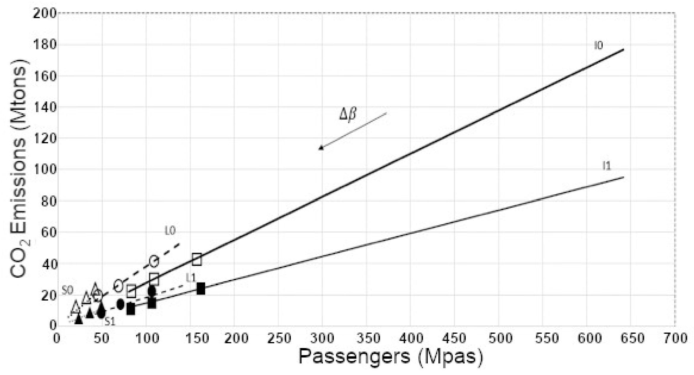
| Case | Name | Distance | CO Production g/Passenger-km |
|---|---|---|---|
| S | National | less than 500 km | 259 |
| L | Intra-European | less than 2500 km | 178 |
| I | Extra-European | less than 5000 km | 114 |
| Irrelevant | Little Relevant | Relevant | Very Relevant |
|---|---|---|---|
| Case | ||||
|---|---|---|---|---|
| S0 | 0.062 | −0.05 | 0.259 | −0.02 |
| S1 | 0.064 | −0.10 | 0.262 | −0.05 |
| L0 | 0.062 | −0.05 | 0.178 | −0.02 |
| L1 | 0.064 | −0.10 | 0.200 | −0.05 |
| I0 | 0.062 | −0.05 | 0.114 | −0.02 |
| I1 | 0.064 | −0.10 | 0.150 | −0.05 |
| National | Intra-European | Extra-European | |
|---|---|---|---|
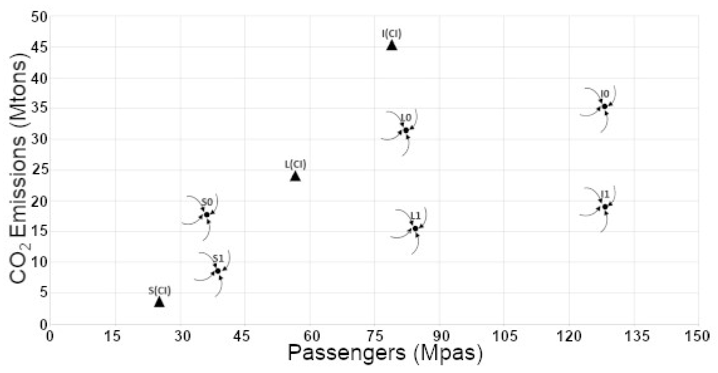
| MPas (CI 1990) | 25.263 | 53.683 | 78.946 |
| MTCO (CI 1990) | 3.27 | 23.89 | 45.00 |
Publisher’s Note: MDPI stays neutral with regard to jurisdictional claims in published maps and institutional affiliations. |
© 2022 by the authors. Licensee MDPI, Basel, Switzerland. This article is an open access article distributed under the terms and conditions of the Creative Commons Attribution (CC BY) license (https://creativecommons.org/licenses/by/4.0/).
Share and Cite
Buendia-Hernandez, F.A.; Ortiz Bevia, M.J.; Alvarez-Garcia, F.J.; Ruizde Elvira, A. Sensitivity of a Dynamic Model of Air Traffic Emissions to Technological and Environmental Factors. Int. J. Environ. Res. Public Health 2022, 19, 15406. https://doi.org/10.3390/ijerph192215406
Buendia-Hernandez FA, Ortiz Bevia MJ, Alvarez-Garcia FJ, Ruizde Elvira A. Sensitivity of a Dynamic Model of Air Traffic Emissions to Technological and Environmental Factors. International Journal of Environmental Research and Public Health. 2022; 19(22):15406. https://doi.org/10.3390/ijerph192215406
Chicago/Turabian StyleBuendia-Hernandez, Francisco A., Maria J. Ortiz Bevia, Francisco J. Alvarez-Garcia, and Antonio Ruizde Elvira. 2022. "Sensitivity of a Dynamic Model of Air Traffic Emissions to Technological and Environmental Factors" International Journal of Environmental Research and Public Health 19, no. 22: 15406. https://doi.org/10.3390/ijerph192215406
APA StyleBuendia-Hernandez, F. A., Ortiz Bevia, M. J., Alvarez-Garcia, F. J., & Ruizde Elvira, A. (2022). Sensitivity of a Dynamic Model of Air Traffic Emissions to Technological and Environmental Factors. International Journal of Environmental Research and Public Health, 19(22), 15406. https://doi.org/10.3390/ijerph192215406