
How Did the Built Environment Affect Urban Vibrancy? A Big Data Approach to Post-Disaster Revitalization Assessment

Abstract
:1. Introduction
2. Materials and Methods
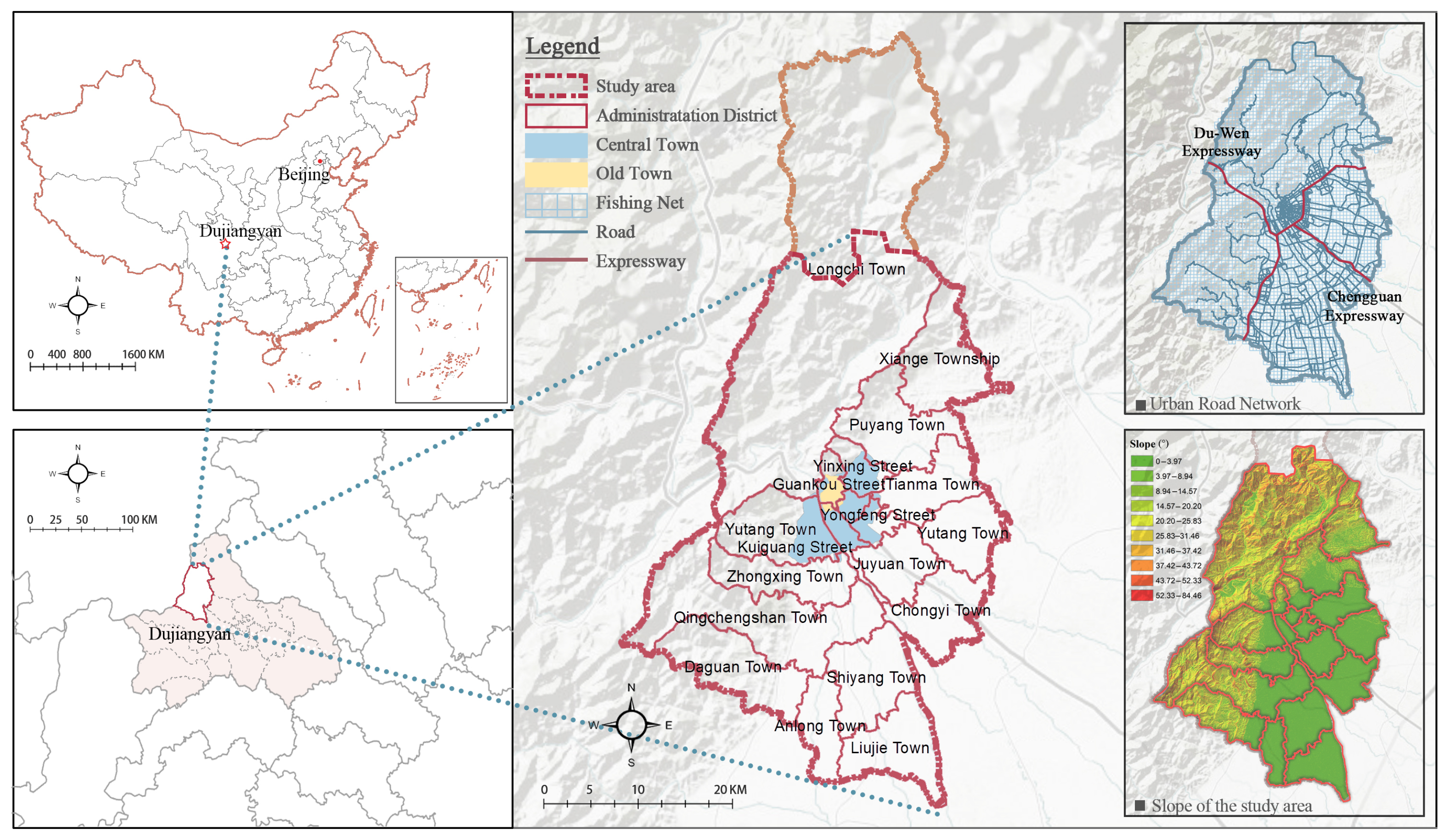
2.1. Study Area
2.2. Data Sources
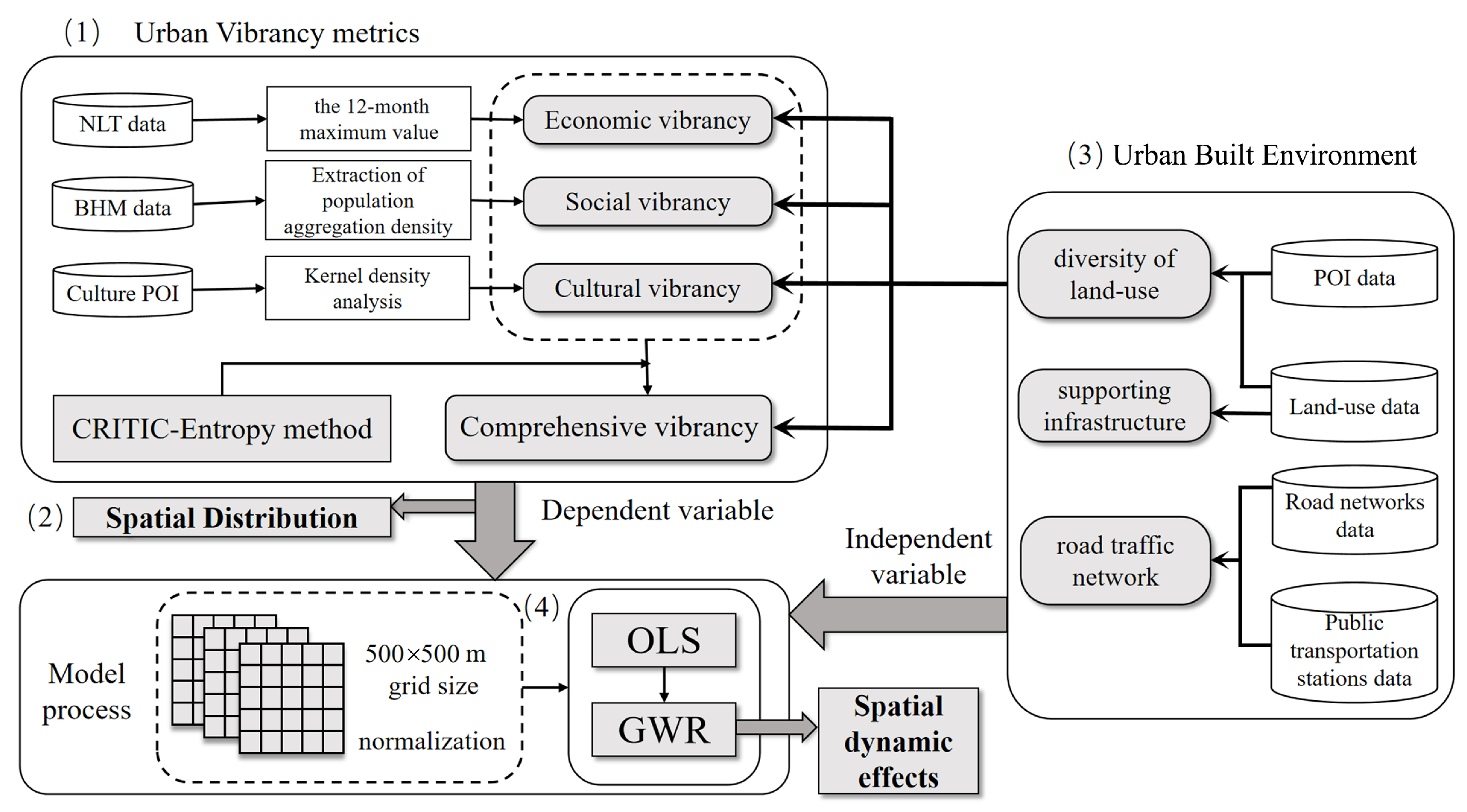
2.3. Methods
2.3.1. Urban Vibrancy Indicators
- (1)
- City Social Vibrancy Index
- (2)
- City Cultural Vibrancy Index
- (3)
- City Economic Vibrancy Index
- (4)
- Comprehensive City Vibrancy Assessment
2.3.2. Built Environment Elements
3. Results
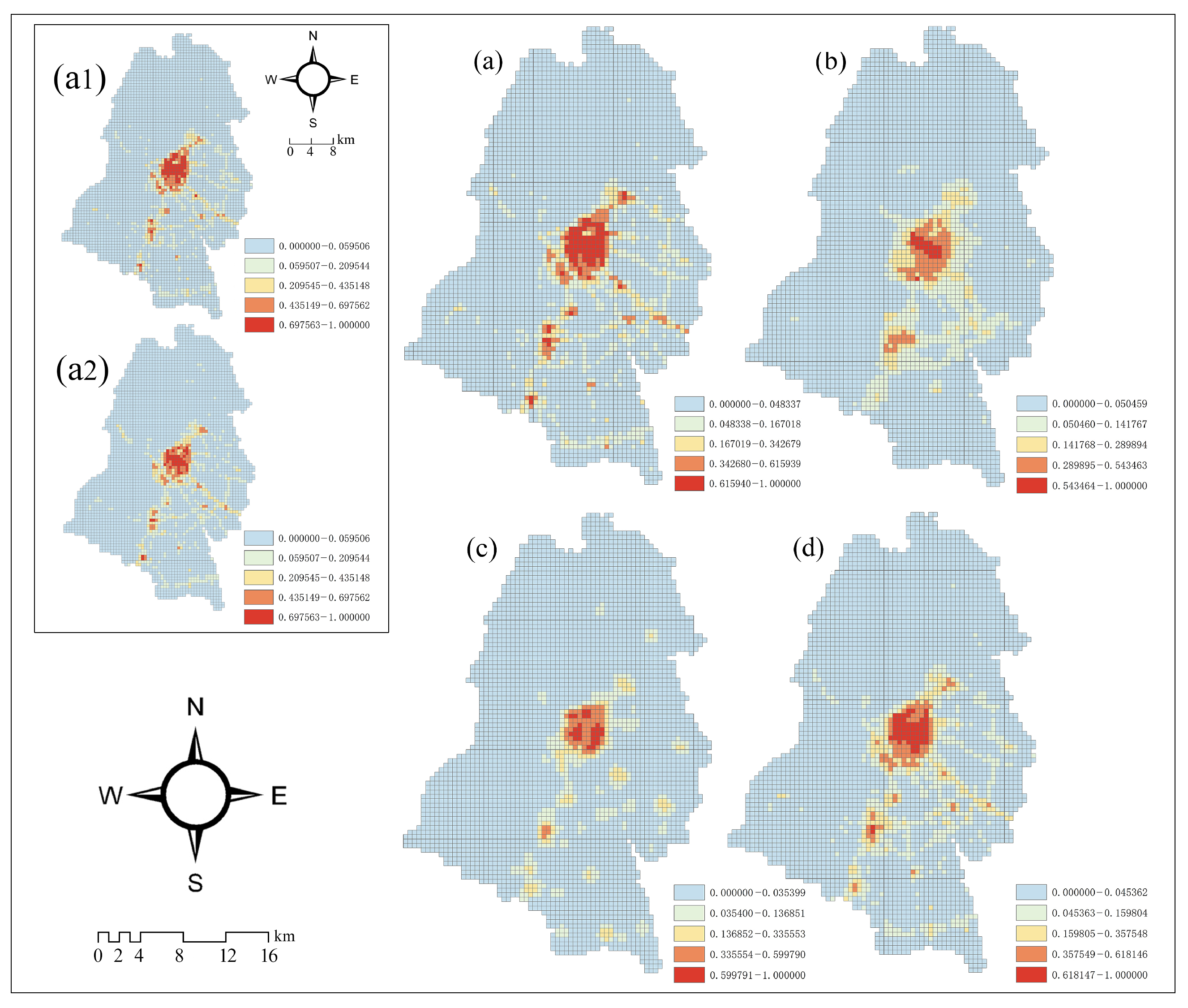
3.1. Spatial Distribution of Urban Vibrancy
3.2. Results of the Global Regression Model
3.3. Results of Geographically Weighted Regression
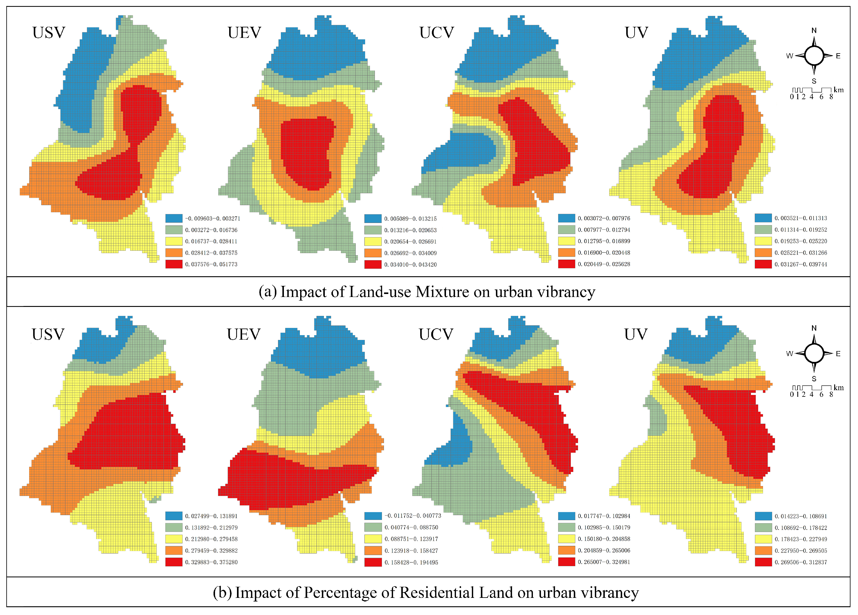
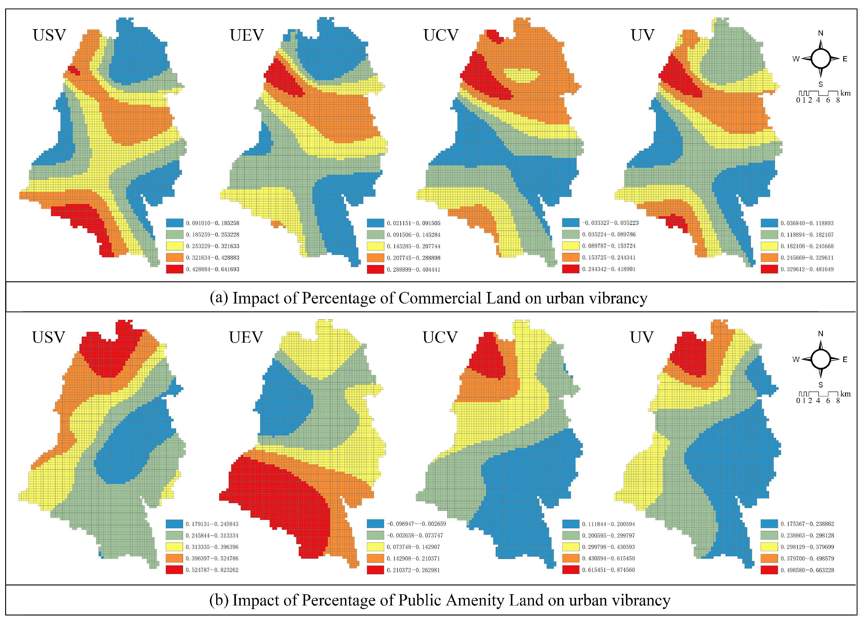
3.3.1. Diversity of Land-Use
3.3.2. Supporting Infrastructure
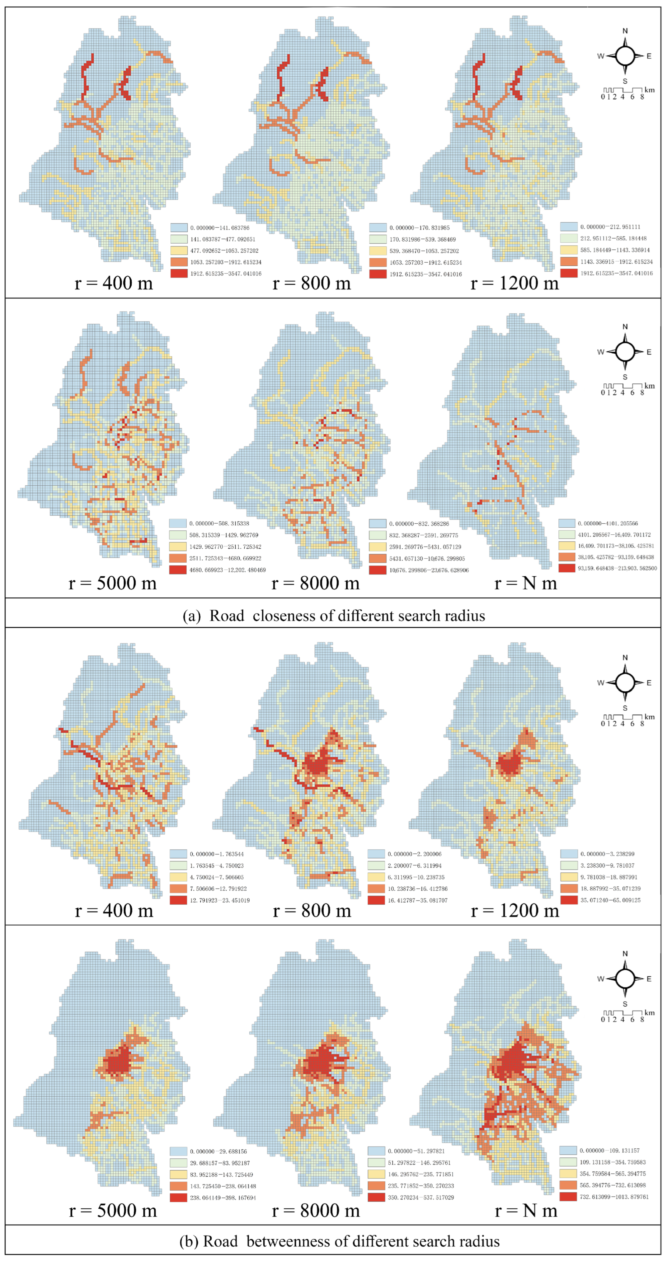
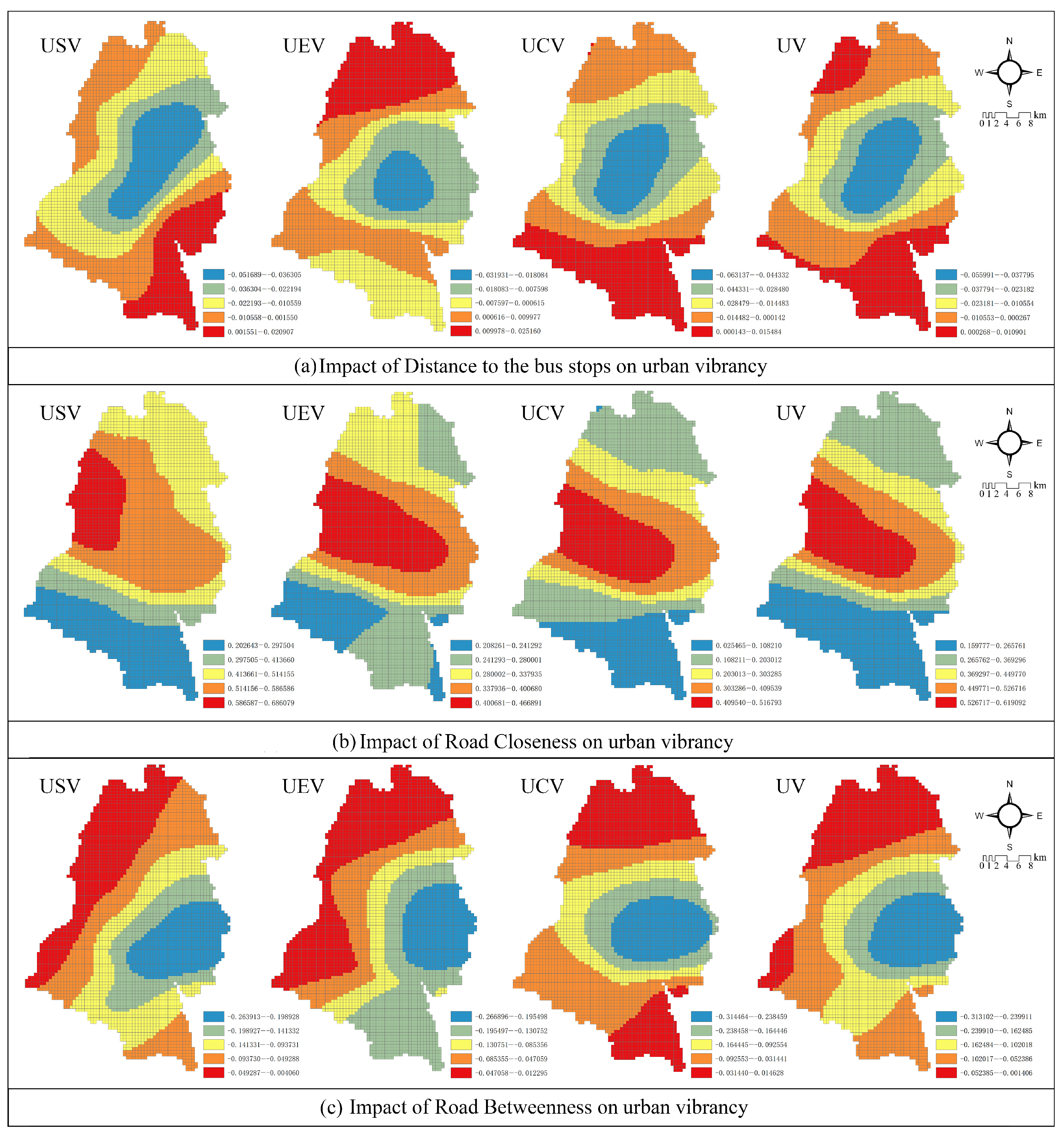
3.3.3. Road Transportation Networks
4. Discussion
4.1. Quantification of Urban Vibrancy and Big Data
4.2. City Vibrancy and Influencing Factors
4.2.1. Spatial Distribution Characteristics of Urban Vibrancy
4.2.2. Linkage between Built Environment Elements and Urban Vibrancy
- (1)
- Diversity of land-use
- (2)
- Supporting infrastructure
- (3)
- Road transportation networks
4.3. Recommendations to Promote Urban Vibrancy
5. Conclusions
Author Contributions
Funding
Institutional Review Board Statement
Data Availability Statement
Acknowledgments
Conflicts of Interest
Abbreviations
| CRITIC | Criteria Importance Though Inter-criteria Correlation |
| BHM | Baidu Heat Map |
| NTL | Nighttime light |
| POI | Point-of-interest |
| Suomi-NPP | The Suomi National Polar-orbiting Partnership |
| VIIRS | The visible infrared imaging radiometer suit |
| GDP | Gross domestic product |
| OLS | Ordinary least squares |
| GWR | Geographically weighted regression |
| GTWR | Geographically and temporally weighted regression |
| USV | Urban Social Vibrancy |
| UEV | Urban Economic Vibrancy |
| UCV | Urban Cultural Vibrancy |
| UV | Urban Comprehensive Vibrancy |
| LMI | Land-use Mixture Index |
| RLI | Residential Land Index |
| CLI | Commercial Land Index |
| PALI | Public Amenity Land Index |
| DI | Distance Index |
| RCI | Road Closeness Index |
| RBI | Road Betweenness Index |
Appendix A

| Integration Category | Specific Type | Counts |
|---|---|---|
| Traffic service | Bus stop/Place name and address information | 2187 |
| Education and culture | Education and culture services/Museums/Libraries/Theatres and concert halls/ Exhibition halls/Scientific research institutions and schools/Place name and address information | 1095 |
| Catering service | Catering services/Place name and address information | 5841 |
| Shopping service | Shopping services/Cars or motorcycle sales/Place name and address information | 10,982 |
| Life service | Life services/Public facilities/Access facilities/Indoor facilities/Place name and address information | 6882 |
| Corporate business | Access facilities/Place name and address information | 2190 |
| Government body | Government agencies/Social organizations/Place name and address information | 1912 |
| Accommodation service | Accommodation services/Place name and address information | 1928 |
| Residential area | Business residence/Place name and address information | 1878 |
| Health care | Health care services/Place name and address information | 1502 |
| Leisure and entertainment | Sports and leisure services/Famous tourist sites/Place name and address information | 1772 |
| Financial service | Financial insurance services/Place name and address information | 431 |
| Variables | Definition | Mean | Standard Deviation | Data Source |
|---|---|---|---|---|
| Land-use Mixture | the Simpson index of the mixed use of 12 POI types | 0.157 | 0.285 | (b) 1 |
| Percentage of Residential Land | The proportion of residential land areas in each unit | 0.031 | 0.119 | (a) 1 |
| Percentage of Commercial Land | The proportion of commercial land areas in each unit | 0.011 | 0.063 | (a) 1 |
| Percentage of Public Amenity Land | The proportion of public amenity land areas in each unit | 0.004 | 0.035 | (a) 1 |
| Road Closeness | a measure of how easy it is for a road to reach other roads within the search radius | 34.370 | 61.333 | (c) 1 |
| Road Betweenness | a measure of the probability of a road segment being passed by traffic flow | 770.402 | 1144.076 | (c) 1 |
| Distance to the bus stops | minimum distance from the grid center point to the nearest bus stop | 180.155 | 261.953 | (d) 1 |
| OLS Models | Coef | Beta Coef | p-Value | R Square | Ajusted R Square |
|---|---|---|---|---|---|
| Model 1 (r = 400) | 0.629860839 | 0.629240989 | |||
| Intercept | 0.000 | 0.842 | |||
| LMI | 0.057 | 0.132 | 0.000 | ||
| RLI | 0.541 | 0.528 | 0.000 | ||
| CLI | 0.437 | 0.216 | 0.000 | ||
| PALI | 0.385 | 0.145 | 0.000 | ||
| DI | −0.007 | −0.017 | 0.098 | ||
| RCI | 0.171 | 0.199 | 0.000 | ||
| RBI | −0.081 | −0.085 | 0.000 | ||
| Model 2 (r = 800) | 0.682883193 | 0.682352136 | |||
| Intercept | −0.004 | 0.025 | |||
| LMI | 0.041 | 0.094 | 0.000 | ||
| RLI | 0.432 | 0.422 | 0.000 | ||
| CLI | 0.362 | 0.179 | 0.000 | ||
| PALI | 0.336 | 0.127 | 0.000 | ||
| DI | −0.022 | −0.049 | 0.000 | ||
| RCI | 0.362 | 0.387 | 0.000 | ||
| RBI | −0.112 | −0.118 | 0.000 | ||
| Model 3 (r = 1200) | 0.716157379 | 0.715682045 | |||
| Intercept | −0.004 | 0.024 | |||
| LMI | 0.032 | 0.075 | 0.000 | ||
| RLI | 0.361 | 0.353 | 0.000 | ||
| CLI | 0.326 | 0.162 | 0.000 | ||
| PALI | 0.294 | 0.111 | 0.000 | ||
| DI | −0.022 | −0.050 | 0.000 | ||
| RCI | 0.503 | 0.474 | 0.000 | ||
| RBI | −0.078 | −0.084 | 0.000 | ||
| Model 4 (r = 5000) | 0.720615665 | 0.720147797 | |||
| Intercept | 0.001 | 0.339 | |||
| LMI | 0.025 | 0.057 | 0.000 | ||
| RLI | 0.343 | 0.335 | 0.000 | ||
| CLI | 0.291 | 0.144 | 0.000 | ||
| PALI | 0.280 | 0.106 | 0.000 | ||
| DI | −0.030 | −0.067 | 0.000 | ||
| RCI | 0.490 | 0.547 | 0.000 | ||
| RBI | −0.163 | −0.111 | 0.000 | ||
| Model 5 (r = 8000) | 0.683390959 | 0.682860752 | |||
| Intercept | 0.000 | 0.825 | |||
| LMI | 0.033 | 0.075 | 0.000 | ||
| RLI | 0.414 | 0.405 | 0.000 | ||
| CLI | 0.329 | 0.163 | 0.000 | ||
| PALI | 0.321 | 0.121 | 0.000 | ||
| DI | −0.033 | −0.075 | 0.000 | ||
| RCI | 0.302 | 0.432 | 0.000 | ||
| RBI | −0.119 | −0.078 | 0.000 | ||
| Model 6 (r = N) | 0.64689031 | 0.646298978 | |||
| Intercept | −0.005 | 0.002 | |||
| LMI | 0.045 | 0.103 | 0.000 | ||
| RLI | 0.498 | 0.486 | 0.000 | ||
| CLI | 0.402 | 0.199 | 0.000 | ||
| PALI | 0.359 | 0.136 | 0.000 | ||
| DI | −0.027 | −0.061 | 0.000 | ||
| RCI | 0.126 | 0.256 | 0.000 | ||
| RBI | 0.023 | 0.010 | 0.323 | ||
| OLS Models (UCV) | Coef | Beta Coef | p-Value | R Square | Ajusted R Square |
|---|---|---|---|---|---|
| Model 1 (r = 400) | 0.558 | 0.557 | |||
| Intercept | 0.000 | ||||
| LMI | 0.038 | 0.137 | 0.000 | ||
| RLI | 0.361 | 0.556 | 0.000 | ||
| CLI | 0.190 | 0.148 | 0.000 | ||
| PALI | 0.270 | 0.161 | 0.000 | ||
| DI | −0.014 | −0.048 | 0.000 | ||
| RCI | 0.044 | 0.080 | 0.000 | ||
| RBI | −0.030 | −0.049 | 0.000 | ||
| Model 2 (r = 800) | 0.601 | 0.600 | |||
| Intercept | −0.002 | 0.057 | |||
| LMI | 0.027 | 0.097 | 0.000 | ||
| RLI | 0.301 | 0.464 | 0.000 | ||
| CLI | 0.145 | 0.113 | 0.000 | ||
| PALI | 0.245 | 0.146 | 0.000 | ||
| DI | −0.026 | −0.093 | 0.000 | ||
| RCI | 0.182 | 0.306 | 0.000 | ||
| RBI | −0.070 | −0.117 | 0.000 | ||
| Model 3 (r = 1200) | 0.658 | 0.658 | |||
| Intercept | −0.003 | 0.010 | |||
| LMI | 0.018 | 0.065 | 0.000 | ||
| RLI | 0.241 | 0.371 | 0.000 | ||
| CLI | 0.110 | 0.085 | 0.000 | ||
| PALI | 0.212 | 0.126 | 0.000 | ||
| DI | −0.031 | −0.109 | 0.000 | ||
| RCI | 0.314 | 0.467 | 0.000 | ||
| RBI | −0.068 | −0.115 | 0.000 | ||
| Model 4 (r = 5000) | 0.668 | 0.668 | |||
| Intercept | 0.001 | 0.440 | |||
| LMI | 0.014 | 0.050 | 0.000 | ||
| RLI | 0.224 | 0.345 | 0.000 | ||
| CLI | 0.082 | 0.064 | 0.000 | ||
| PALI | 0.203 | 0.121 | 0.000 | ||
| DI | −0.034 | −0.121 | 0.000 | ||
| RCI | 0.325 | 0.573 | 0.000 | ||
| RBI | −0.164 | −0.175 | 0.000 | ||
| Model 5 (r = 8000) | 0.610 | 0.609 | |||
| Intercept | −0.001 | 0.540 | |||
| LMI | 0.021 | 0.078 | 0.000 | ||
| RLI | 0.284 | 0.437 | 0.000 | ||
| CLI | 0.119 | 0.093 | 0.000 | ||
| PALI | 0.237 | 0.141 | 0.000 | ||
| DI | −0.033 | −0.117 | 0.000 | ||
| RCI | 0.174 | 0.391 | 0.000 | ||
| RBI | −0.113 | −0.118 | 0.000 | ||
| Model 6 (r = N) | 0.569 | 0.568 | |||
| Intercept | −0.003 | 0.024 | |||
| LMI | 0.031 | 0.113 | 0.000 | ||
| RLI | 0.341 | 0.526 | 0.000 | ||
| CLI | 0.172 | 0.134 | 0.000 | ||
| PALI | 0.260 | 0.155 | 0.000 | ||
| DI | −0.025 | −0.087 | 0.000 | ||
| RCI | 0.049 | 0.156 | 0.000 | ||
| RBI | 0.007 | 0.005 | 0.679 | ||
| OLS Models(UEV) | Coef | Beta Coef | p-Value | R Square | Ajusted R Square |
|---|---|---|---|---|---|
| Model 1 (r = 400) | 0.567 | 0.567 | |||
| Intercept | 0.010 | 0.000 | |||
| LMI | 0.048 | 0.177 | 0.000 | ||
| RLI | 0.288 | 0.452 | 0.000 | ||
| CLI | 0.282 | 0.224 | 0.000 | ||
| PALI | 0.236 | 0.143 | 0.000 | ||
| DI | 0.006 | 0.022 | 0.048 | ||
| RCI | 0.089 | 0.167 | 0.000 | ||
| RBI | −0.050 | −0.085 | 0.000 | ||
| Model 2 (r = 800) | 0.608 | 0.608 | |||
| Intercept | 0.008 | 0.000 | |||
| LMI | 0.039 | 0.144 | 0.000 | ||
| RLI | 0.229 | 0.360 | 0.000 | ||
| CLI | 0.242 | 0.192 | 0.000 | ||
| PALI | 0.209 | 0.127 | 0.000 | ||
| DI | −0.002 | −0.008 | 0.457 | ||
| RCI | 0.196 | 0.336 | 0.000 | ||
| RBI | −0.069 | −0.117 | 0.000 | ||
| Model 3 (r = 1200) | 0.653 | 0.652 | |||
| Intercept | 0.008 | 0.000 | |||
| LMI | 0.032 | 0.119 | 0.000 | ||
| RLI | 0.178 | 0.280 | 0.000 | ||
| CLI | 0.213 | 0.170 | 0.000 | ||
| PALI | 0.181 | 0.110 | 0.000 | ||
| DI | −0.004 | −0.016 | 0.091 | ||
| RCI | 0.304 | 0.460 | 0.000 | ||
| RBI | −0.059 | −0.101 | 0.000 | ||
| Model 4 (r = 5000) | 0.695 | 0.695 | |||
| Intercept | 0.011 | 0.000 | |||
| LMI | 0.024 | 0.087 | 0.000 | ||
| RLI | 0.144 | 0.226 | 0.000 | ||
| CLI | 0.173 | 0.137 | 0.000 | ||
| PALI | 0.162 | 0.098 | 0.000 | ||
| DI | −0.013 | −0.046 | 0.000 | ||
| RCI | 0.351 | 0.629 | 0.000 | ||
| RBI | −0.145 | −0.158 | 0.000 | ||
| Model 5 (r = 8000) | 0.655 | 0.655 | |||
| Intercept | 0.009 | 0.000 | |||
| LMI | 0.028 | 0.105 | 0.000 | ||
| RLI | 0.190 | 0.298 | 0.000 | ||
| CLI | 0.194 | 0.155 | 0.000 | ||
| PALI | 0.191 | 0.116 | 0.000 | ||
| DI | −0.016 | −0.058 | 0.000 | ||
| RCI | 0.230 | 0.527 | 0.000 | ||
| RBI | −0.140 | −0.148 | 0.000 | ||
| Model 6 (r = N) | 0.589 | 0.588 | |||
| Intercept | 0.006 | 0.000 | |||
| LMI | 0.039 | 0.145 | 0.000 | ||
| RLI | 0.260 | 0.408 | 0.000 | ||
| CLI | 0.259 | 0.206 | 0.000 | ||
| PALI | 0.220 | 0.134 | 0.000 | ||
| DI | −0.008 | −0.029 | 0.010 | ||
| RCI | 0.075 | 0.246 | 0.000 | ||
| RBI | 0.018 | 0.013 | 0.230 | ||
| OLS Models | Coef | Beta Coef | p-Value | R Square | Ajusted R Square |
|---|---|---|---|---|---|
| Model 1 (r = 400) | 0.655 | 0.654 | |||
| Intercept | 0.003 | 0.013 | |||
| LMI | 0.053 | 0.154 | 0.000 | ||
| RLI | 0.448 | 0.551 | 0.000 | ||
| CLI | 0.328 | 0.205 | 0.000 | ||
| PALI | 0.335 | 0.160 | 0.000 | ||
| DI | −0.007 | −0.020 | 0.040 | ||
| RCI | 0.107 | 0.156 | 0.000 | ||
| RBI | −0.057 | −0.076 | 0.000 | ||
| Model 2 (r = 800) | 0.708 | 0.708 | |||
| Intercept | 0.000 | 0.761 | |||
| LMI | 0.039 | 0.114 | 0.000 | ||
| RLI | 0.364 | 0.448 | 0.000 | ||
| CLI | 0.269 | 0.168 | 0.000 | ||
| PALI | 0.298 | 0.142 | 0.000 | ||
| DI | −0.021 | −0.058 | 0.000 | ||
| RCI | 0.271 | 0.365 | 0.000 | ||
| RBI | −0.093 | −0.124 | 0.000 | ||
| Model 3 (r = 1200) | 0.760 | 0.759 | |||
| Intercept | 9.172 0.000 | 0.937 | |||
| LMI | 0.030 | 0.087 | 0.000 | ||
| RLI | 0.294 | 0.362 | 0.000 | ||
| CLI | 0.230 | 0.144 | 0.000 | ||
| PALI | 0.259 | 0.124 | 0.000 | ||
| DI | −0.024 | −0.067 | 0.000 | ||
| RCI | 0.418 | 0.497 | 0.000 | ||
| RBI | −0.078 | −0.106 | 0.000 | ||
| Model 4 (r = 5000) | 0.777 | 0.777 | |||
| Intercept | 0.004 | 0.000 | |||
| LMI | 0.023 | 0.066 | 0.000 | ||
| RLI | 0.268 | 0.330 | 0.000 | ||
| CLI | 0.192 | 0.120 | 0.000 | ||
| PALI | 0.244 | 0.116 | 0.000 | ||
| DI | −0.031 | −0.087 | 0.000 | ||
| RCI | 0.435 | 0.612 | 0.000 | ||
| RBI | −0.181 | −0.155 | 0.000 | ||
| Model 5 (r = 8000) | 0.725 | 0.724 | |||
| Intercept | 0.003 | 0.023 | |||
| LMI | 0.030 | 0.089 | 0.000 | ||
| RLI | 0.336 | 0.414 | 0.000 | ||
| CLI | 0.229 | 0.143 | 0.000 | ||
| PALI | 0.283 | 0.135 | 0.000 | ||
| DI | −0.032 | −0.091 | 0.000 | ||
| RCI | 0.260 | 0.467 | 0.000 | ||
| RBI | −0.141 | −0.117 | 0.000 | ||
| Model 6 (r = N) | 0.673 | 0.673 | |||
| Intercept | −0.001 | 0.455 | |||
| LMI | 0.043 | 0.125 | 0.000 | ||
| RLI | 0.415 | 0.511 | 0.000 | ||
| CLI | 0.301 | 0.188 | 0.000 | ||
| PALI | 0.317 | 0.151 | 0.000 | ||
| DI | −0.024 | −0.066 | 0.000 | ||
| RCI | 0.090 | 0.230 | 0.000 | ||
| RBI | 0.017 | 0.009 | 0.337 | ||
References
- March, A.; Rijal, Y.; Wilkinson, S.; Firidin Özgür, E. Measuring building adaptability and street vitality. Plan. Pract. Res. 2012, 27, 531–552. [Google Scholar] [CrossRef]
- Row, A.T. The death and life of great american cities. Yale Law J. 1962, 71, 1597–1602. [Google Scholar] [CrossRef]
- Gehl, J.; Mortensen, L. Livet Mellem Husene: Udeaktiviteter og Udemiljøer; China Construction Industry Press: Beijing, China, 2002. [Google Scholar]
- Montgomery, J. Making a city: Urbanity, vitality and urban design. J. Urban Des. 1998, 3, 93–116. [Google Scholar] [CrossRef]
- Fu, R.; Zhang, X.; Yang, D.; Cai, T.; Zhang, Y. The relationship between urban vibrancy and built environment: An empirical study from an emerging city in an Arid Region. Int. J. Environ. Res. Public Health 2021, 18, 525. [Google Scholar] [CrossRef]
- Lu, S.; Shi, C.; Yang, X. Impacts of built environment on urban vitality: Regression analyses of Beijing and Chengdu, China. Int. J. Environ. Res. Public Health 2019, 16, 4592. [Google Scholar] [CrossRef]
- Li, X.; Qian, Y.; Zeng, J.; Wei, X.; Guang, X. The Influence of Strip-City Street Network Structure on Spatial Vitality: Case Studies in Lanzhou, China. Land 2021, 10, 1107. [Google Scholar] [CrossRef]
- Wang, X.; Zhang, Y.; Yu, D.; Qi, J.; Li, S. Investigating the spatiotemporal pattern of urban vibrancy and its determinants: Spatial big data analyses in Beijing, China. Land Use Policy 2022, 119, 106162. [Google Scholar] [CrossRef]
- Liu, S.; Zhang, L.; Long, Y. Urban vitality area identification and pattern analysis from the perspective of time and space fusion. Sustainability 2019, 11, 4032. [Google Scholar] [CrossRef]
- Wu, C.; Ye, X.; Ren, F.; Du, Q. Check-in behaviour and spatio-temporal vibrancy: An exploratory analysis in Shenzhen, China. Cities 2018, 77, 104–116. [Google Scholar] [CrossRef]
- Li, Q.; Cui, C.; Liu, F.; Wu, Q.; Run, Y.; Han, Z. Multidimensional urban vitality on streets: Spatial patterns and influence factor identification using multisource urban data. ISPRS Int. J. Geo-Inf. 2022, 11, 2. [Google Scholar] [CrossRef]
- Feng, D.; Tu, L.; Sun, Z. Research on population spatiotemporal aggregation characteristics of a small city: A case study on Shehong County based on Baidu heat maps. Sustainability 2019, 11, 6276. [Google Scholar] [CrossRef]
- Shi, P.; Xiao, Y.; Zhan, Q. A study on spatial and temporal aggregation patterns of urban population in Wuhan City based on Baidu heat map and POI data. Int. Rev. Spat. Plan. Sustain. Dev. 2020, 8, 101–121. [Google Scholar] [CrossRef]
- Zhang, S.; Zhang, W.; Wang, Y.; Zhao, X.; Song, P.; Tian, G.; Mayer, A.L. Comparing human activity density and green space supply using the Baidu Heat Map in Zhengzhou, China. Sustainability 2020, 12, 7075. [Google Scholar] [CrossRef]
- Xu, G.; Su, J.; Xia, C.; Li, X.; Xiao, R. Spatial mismatches between nighttime light intensity and building morphology in Shanghai, China. Sustain. Cities Soc. 2022, 81, 103851. [Google Scholar] [CrossRef]
- Liu, S.; Zhang, L.; Long, Y.; Long, Y.; Xu, M. A new urban vitality analysis and evaluation framework based on human activity modeling using multi-source big data. ISPRS Int. J. Geo-Inf. 2020, 9, 617. [Google Scholar] [CrossRef]
- Liu, Y.; Liu, X.; Gao, S.; Gong, L.; Kang, C.; Zhi, Y.; Chi, G.; Shi, L. Social sensing: A new approach to understanding our socioeconomic environments. Ann. Assoc. Am. Geogr. 2015, 105, 512–530. [Google Scholar] [CrossRef]
- Botta, F.; Gutiérrez-Roig, M. Modelling urban vibrancy with mobile phone and OpenStreetMap data. PloS ONE 2021, 16, e0252015. [Google Scholar] [CrossRef]
- Wu, J.; Ta, N.; Song, Y.; Lin, J.; Chai, Y. Urban form breeds neighborhood vibrancy: A case study using a GPS-based activity survey in suburban Beijing. Cities 2018, 74, 100–108. [Google Scholar] [CrossRef]
- Meng, Y.; Xing, H. Exploring the relationship between landscape characteristics and urban vibrancy: A case study using morphology and review data. Cities 2019, 95, 102389. [Google Scholar] [CrossRef]
- Jiang, Y.; Chen, Z.; Sun, P. Urban Shrinkage and Urban Vitality Correlation Research in the Three Northeastern Provinces of China. Int. J. Environ. Res. Public Health 2022, 19, 10650. [Google Scholar] [CrossRef]
- Tu, W.; Zhu, T.; Xia, J.; Zhou, Y.; Lai, Y.; Jiang, J.; Li, Q. Portraying the spatial dynamics of urban vibrancy using multisource urban big data. Comput. Environ. Urban Syst. 2020, 80, 101428. [Google Scholar] [CrossRef]
- Mpogas, K.; Kopelias, P.; Mitropoulos, L.; Kepaptsoglou, K. Road safety in urban areas in Greece during economy downturn. A before–after comparison. Transp. Res. Procedia 2017, 24, 228–234. [Google Scholar] [CrossRef]
- Huang, B.; Zhou, Y.; Li, Z.; Song, Y.; Cai, J.; Tu, W. Evaluating and characterizing urban vibrancy using spatial big data: Shanghai as a case study. Environ. Plan. B Urban Anal. City Sci. 2020, 47, 1543–1559. [Google Scholar] [CrossRef]
- Bastani, M.; Damgacioglu, H.; Celik, N. A δ-constraint multi-objective optimization framework for operation planning of smart grids. Sustain. Cities Soc. 2018, 38, 21–30. [Google Scholar] [CrossRef]
- Xu, H.; Wang, L.; Li, Y.; Huang, L.; Yin, L. Critical Chinese government behavior for swift housing reconstruction programme—The case of Dujiangyan following Wenchuan Earthquake. Int. J. Disaster Risk Reduct. 2019, 41, 101307. [Google Scholar] [CrossRef]
- Chen, Y.; Song, J.; Zhong, S.; Liu, Z.; Gao, W. Effect of destructive earthquake on the population-economy-space urbanization at county level-a case study on Dujiangyan county, China. Sustain. Cities Soc. 2022, 76, 103345. [Google Scholar] [CrossRef]
- Wang, B.; Lei, Y.; Xue, D.; Liu, J.; Wei, C. Elaborating Spatiotemporal Associations Between the Built Environment and Urban Vibrancy: A Case of Guangzhou City, China. Chin. Geogr. Sci. 2022, 32, 480–492. [Google Scholar] [CrossRef]
- Wirth, L. “Urbanism as a Way of Life”: American Journal of Sociology (1938). In The City Reader; Routledge: London, UK, 2011; pp. 128–136. [Google Scholar]
- Zhang, H. Extracting Active Population Data Based on Baidu Heat Maps for Transportation Planning Applications. Urban Transp. 2021, 19, 103–111. [Google Scholar] [CrossRef]
- Fan, D.; Qin, K.; Kang, C. Understanding Urban Functionality from POI Space. In Proceedings of the 2018 26th International Conference on Geoinformatics, IEEE, Kunming, China, 28–30 June 2018; pp. 1–6. [Google Scholar]
- Xie, Z.; Yan, J. Kernel density estimation of traffic accidents in a network space. Comput. Environ. Urban Syst. 2008, 32, 396–406. [Google Scholar] [CrossRef]
- Levin, N.; Kyba, C.C.; Zhang, Q.; de Miguel, A.S.; Román, M.O.; Li, X.; Portnov, B.A.; Molthan, A.L.; Jechow, A.; Miller, S.D.; et al. Remote sensing of night lights: A review and an outlook for the future. Remote Sens. Environ. 2020, 237, 111443. [Google Scholar] [CrossRef]
- Zhang, Y.; Shang, K.; Shi, Z.; Wang, H.; Li, X. Spatial pattern of the vitality of Chinese characteristic towns: A perspective from nighttime lights. Land 2022, 11, 85. [Google Scholar] [CrossRef]
- Elvidge, C.D.; Baugh, K.E.; Anderson, S.J.; Sutton, P.C.; Ghosh, T. The Night Light Development Index (NLDI): A spatially explicit measure of human development from satellite data. Soc. Geogr. 2012, 7, 23–35. [Google Scholar] [CrossRef]
- Tu, W.; Zhu, T.; Zhong, C.; Zhang, X.; Xu, Y.; Li, Q. Exploring metro vibrancy and its relationship with built environment: A cross-city comparison using multi-source urban data. Geo-Spat. Inf. Sci. 2022, 25, 182–196. [Google Scholar] [CrossRef]
- Diakoulaki, D.; Mavrotas, G.; Papayannakis, L. Determing objective weights in multiple criteria problems: The CRITIC method. Comput. Oper. Res. 1995, 22, 763–770. [Google Scholar] [CrossRef]
- Kumar, R.; Singh, S.; Bilga, P.S.; Jatin; Singh, J.; Singh, S.; Scutaru, M.L.; Pruncu, C.I. Revealing the benefits of entropy weights method for multi-objective optimization in machining operations: A critical review. J. Mater. Res. Technol. 2021, 10, 1471–1492. [Google Scholar] [CrossRef]
- Li, F.; Su, M.; Li, D. Combination Evaluation Model Based on Entropy Weight Method. In Proceedings of the ICMLCA 2021; 2nd International Conference on Machine Learning and Computer Application, Shenyang, China, 17–19 December 2021; pp. 1–5. [Google Scholar]
- Pan, C.; Zhou, J.; Huang, X. Impact of Check-In Data on Urban Vitality in the Macao Peninsula. Sci. Program. 2021, 2021, 7179965. [Google Scholar] [CrossRef]
- Tang, L.; Lin, Y.; Li, S.; Li, S.; Li, J.; Ren, F.; Wu, C. Exploring the influence of urban form on urban vibrancy in shenzhen based on mobile phone data. Sustainability 2018, 10, 4565. [Google Scholar] [CrossRef]
- Hillier, B. Space is the Machine: A Configurational Theory of Architecture; Space Syntax: London, UK, 2007. [Google Scholar]
- Barmpounakis, E.; Geroliminis, N. On the new era of urban traffic monitoring with massive drone data: The pNEUMA large-scale field experiment. Transp. Res. Part C Emerg. Technol. 2020, 111, 50–71. [Google Scholar] [CrossRef]
- Kandt, J.; Batty, M. Smart cities, big data and urban policy: Towards urban analytics for the long run. Cities 2021, 109, 102992. [Google Scholar] [CrossRef]
- Lan, F.; Gong, X.; Da, H.; Wen, H. How do population inflow and social infrastructure affect urban vitality? Evidence from 35 large-and medium-sized cities in China. Cities 2020, 100, 102454. [Google Scholar] [CrossRef]
- Lv, G.; Zheng, S.; Hu, W. Exploring the relationship between the built environment and block vitality based on multi-source big data: An analysis in Shenzhen, China. Geomat. Nat. Hazards Risk 2022, 13, 1593–1613. [Google Scholar] [CrossRef]
- Lu, H.; Zhao, Y.; Zhou, X.; Wei, Z. Selection of agricultural machinery based on improved CRITIC-entropy weight and GRA-TOPSIS method. Processes 2022, 10, 266. [Google Scholar] [CrossRef]
- Wu, Z.; Guan, J.; He, J. An empirical study on the calculation of minimum wage standard—Dynamic combination calculation based on objective weight of CRITIC-Entropy Weight Method. Mod. Econ. Sci. 2019, 41, 103–117. [Google Scholar]
- Zafar, S.; Alamgir, Z.; Rehman, M. An effective blockchain evaluation system based on entropy-CRITIC weight method and MCDM techniques. Peer-to-Peer Netw. Appl. 2021, 14, 3110–3123. [Google Scholar] [CrossRef]
- Zheng, Y.; Liu, T.; Wang, Y.; Zhu, Y.; Liu, Y.; Chang, E. Diagnosing New York city’s noises with ubiquitous data. In Proceedings of the 2014 ACM International Joint Conference on Pervasive and Ubiquitous Computing, Seattle, WA, USA, 13–17 September 2014; pp. 715–725. [Google Scholar]
- Li, Q.; Umaier, K.; Koide, O. Research on post-Wenchuan earthquake recovery and reconstruction implementation: A case study of housing reconstruction of Dujiangyan City. Prog. Disaster Sci. 2019, 4, 100041. [Google Scholar] [CrossRef]
- Yin, H.; Kong, F.; Zhang, X. Changes of residential land density and spatial pattern from 1989 to 2004 in Jinan City, China. Chin. Geogr. Sci. 2011, 21, 619–628. [Google Scholar] [CrossRef]
- He, Q.; He, W.; Song, Y.; Wu, J.; Yin, C.; Mou, Y. The impact of urban growth patterns on urban vitality in newly built-up areas based on an association rules analysis using geographical ‘big data’. Land Use Policy 2018, 78, 726–738. [Google Scholar] [CrossRef]
- Jin, X.; Long, Y.; Sun, W.; Lu, Y.; Yang, X.; Tang, J. Evaluating cities’ vitality and identifying ghost cities in China with emerging geographical data. Cities 2017, 63, 98–109. [Google Scholar] [CrossRef]
- Yue, Y.; Zhuang, Y.; Yeh, A.G.; Xie, J.Y.; Ma, C.L.; Li, Q.Q. Measurements of POI-based mixed use and their relationships with neighbourhood vibrancy. Int. J. Geogr. Inf. Sci. 2017, 31, 658–675. [Google Scholar] [CrossRef] [Green Version]


| Index | Abbreviation | Mean | Standard Deviation |
|---|---|---|---|
| Land-use Mixture Index | LMI | 0.17615635 | 0.31882732 |
| Residential Land Index | RLI | 0.03536129 | 0.13483714 |
| Commercial Land Index | CLI | 0.01238231 | 0.06834059 |
| Public Amenity Land Index | PALI | 0.00598902 | 0.05220615 |
| Distance Index | DI | 0.21211727 | 0.30846335 |
| Road Closeness Index | RCI | 0.08632102 | 0.15405602 |
| Road Betweenness Index | RBI | 0.06313485 | 0.09376886 |
| OLS Models | Coef | Beta Coef | p-Value | Std. | Vif | R Square | Adjusted R Square | AICc |
|---|---|---|---|---|---|---|---|---|
| Model 1 (USV) 1 | 0.721 | 0.720 | −10,023.679 | |||||
| Intercept | 0.001 | 0.339 | 0.005 | |||||
| RLI | 0.343 | 0.335 | 0.000 | 0.074 | 1.661 | |||
| CLI | 0.291 | 0.144 | 0.000 | 0.097 | 1.163 | |||
| PALI | 0.280 | 0.106 | 0.000 | 0.113 | 1.079 | |||
| DI | −0.030 | −0.067 | 0.000 | 0.017 | 1.142 | |||
| RCI | 0.490 | 0.547 | 0.000 | 0.131 | 2.966 | |||
| RBI | −0.163 | −0.111 | 0.000 | 0.071 | 1.696 | |||
| Model 2 (UCV) 1 | 0.668 | 0.668 | −13,120.566 | |||||
| Intercept | 0.001 | 0.440 | 0.004 | |||||
| LMI | 0.014 | 0.050 | 0.000 | 0.006 | 1.357 | |||
| RLI | 0.224 | 0.345 | 0.000 | 0.072 | 1.661 | |||
| CLI | 0.082 | 0.064 | 0.000 | 0.084 | 1.163 | |||
| PALI | 0.203 | 0.121 | 0.000 | 0.148 | 1.079 | |||
| DI | −0.034 | −0.121 | 0.000 | 0.020 | 1.142 | |||
| RCI | 0.325 | 0.573 | 0.000 | 0.142 | 2.966 | |||
| RBI | −0.164 | −0.175 | 0.000 | 0.097 | 1.696 | |||
| Model 3 (UEV) 1 | 0.695 | 0.695 | −13,626.702 | |||||
| Intercept | 0.011 | 0.000 | 0.004 | |||||
| LMI | 0.024 | 0.087 | 0.000 | 0.009 | 1.357 | |||
| RLI | 0.144 | 0.226 | 0.000 | 0.056 | 1.661 | |||
| CLI | 0.173 | 0.137 | 0.000 | 0.072 | 1.163 | |||
| PALI | 0.162 | 0.098 | 0.000 | 0.096 | 1.079 | |||
| DI | −0.013 | −0.046 | 0.000 | 0.012 | 1.142 | |||
| RCI | 0.351 | 0.629 | 0.000 | 0.074 | 2.966 | |||
| RBI | −0.145 | −0.158 | 0.000 | 0.073 | 1.696 | |||
| Model 4 (UV) 1 | 0.777 | 0.776 | −12,905.897 | |||||
| Intercept | 0.004 | 0.000 | 0.003 | |||||
| LMI | 0.023 | 0.066 | 0.000 | 0.009 | 1.357 | |||
| RLI | 0.268 | 0.330 | 0.000 | 0.060 | 1.661 | |||
| CLI | 0.192 | 0.120 | 0.000 | 0.080 | 1.163 | |||
| PALI | 0.244 | 0.116 | 0.000 | 0.092 | 1.079 | |||
| DI | −0.031 | −0.087 | 0.000 | 0.017 | 1.142 | |||
| RCI | 0.435 | 0.612 | 0.000 | 0.131 | 2.966 | |||
| RBI | −0.181 | −0.155 | 0.000 | 0.087 | 1.696 | |||
| GWR Models | Min | Median | Max | Mean | R Square | Adjusted R Square | AICc |
|---|---|---|---|---|---|---|---|
| Model 1 (USV) | 0.758 | 0.756 | −10,578.473 | ||||
| Intercept | −0.021 | 0.000 | 0.007 | −0.001 | |||
| LMI | −0.010 | 0.028 | 0.052 | 0.024 | |||
| RLI | 0.027 | 0.292 | 0.375 | 0.278 | |||
| CLI | 0.091 | 0.262 | 0.642 | 0.267 | |||
| PALI | 0.179 | 0.293 | 0.823 | 0.333 | |||
| DI | −0.052 | −0.014 | 0.021 | −0.016 | |||
| RCI | 0.203 | 0.498 | 0.686 | 0.455 | |||
| RBI | −0.264 | −0.093 | −0.004 | −0.106 | |||
| Model 2 (UCV) | 0.748 | 0.745 | −14,210.057 | ||||
| Intercept | −0.018 | 0.000 | 0.005 | −0.001 | |||
| LMI | 0.003 | 0.015 | 0.026 | 0.014 | |||
| RLI | 0.018 | 0.166 | 0.325 | 0.180 | |||
| CLI | −0.033 | 0.098 | 0.419 | 0.110 | |||
| PALI | 0.112 | 0.238 | 0.875 | 0.281 | |||
| DI | −0.063 | −0.015 | 0.015 | −0.017 | |||
| RCI | 0.025 | 0.226 | 0.517 | 0.250 | |||
| RBI | −0.314 | −0.069 | 0.015 | −0.102 | |||
| Model 3 (UEV) | 0.744 | 0.741 | −14,307.063 | ||||
| Intercept | 0.007 | 0.011 | 0.026 | 0.012 | |||
| LMI | 0.005 | 0.022 | 0.043 | 0.022 | |||
| RLI | −0.012 | 0.110 | 0.194 | 0.107 | |||
| CLI | 0.021 | 0.131 | 0.404 | 0.142 | |||
| PALI | −0.097 | 0.111 | 0.263 | 0.118 | |||
| DI | −0.032 | 0.000 | 0.025 | −0.001 | |||
| RCI | 0.208 | 0.304 | 0.467 | 0.323 | |||
| RBI | −0.267 | −0.086 | −0.012 | −0.104 | |||
| Model 4 (UV) | 0.825 | 0.823 | −13,864.880 | ||||
| Intercept | −0.009 | 0.003 | 0.011 | 0.003 | |||
| LMI | 0.004 | 0.023 | 0.040 | 0.022 | |||
| RLI | 0.014 | 0.216 | 0.313 | 0.213 | |||
| CLI | 0.037 | 0.171 | 0.482 | 0.188 | |||
| PALI | 0.175 | 0.260 | 0.663 | 0.285 | |||
| DI | −0.056 | −0.010 | 0.011 | −0.014 | |||
| RCI | 0.160 | 0.367 | 0.619 | 0.377 | |||
| RBI | −0.313 | −0.097 | −0.001 | −0.119 | |||
Publisher’s Note: MDPI stays neutral with regard to jurisdictional claims in published maps and institutional affiliations. |
© 2022 by the authors. Licensee MDPI, Basel, Switzerland. This article is an open access article distributed under the terms and conditions of the Creative Commons Attribution (CC BY) license (https://creativecommons.org/licenses/by/4.0/).
Share and Cite
Gong, H.; Wang, X.; Wang, Z.; Liu, Z.; Li, Q.; Zhang, Y. How Did the Built Environment Affect Urban Vibrancy? A Big Data Approach to Post-Disaster Revitalization Assessment. Int. J. Environ. Res. Public Health 2022, 19, 12178. https://doi.org/10.3390/ijerph191912178
Gong H, Wang X, Wang Z, Liu Z, Li Q, Zhang Y. How Did the Built Environment Affect Urban Vibrancy? A Big Data Approach to Post-Disaster Revitalization Assessment. International Journal of Environmental Research and Public Health. 2022; 19(19):12178. https://doi.org/10.3390/ijerph191912178
Chicago/Turabian StyleGong, Hongyu, Xiaozihan Wang, Zihao Wang, Ziyi Liu, Qiushan Li, and Yunhan Zhang. 2022. "How Did the Built Environment Affect Urban Vibrancy? A Big Data Approach to Post-Disaster Revitalization Assessment" International Journal of Environmental Research and Public Health 19, no. 19: 12178. https://doi.org/10.3390/ijerph191912178