
Territorial Pattern Evolution and Its Comprehensive Carrying Capacity Evaluation in the Coastal Area of Beibu Gulf, China

Abstract
:1. Introduction
2. Materials and Methods
2.1. The Study Area
2.2. Data Sources
2.3. Territorial Pattern Analysis
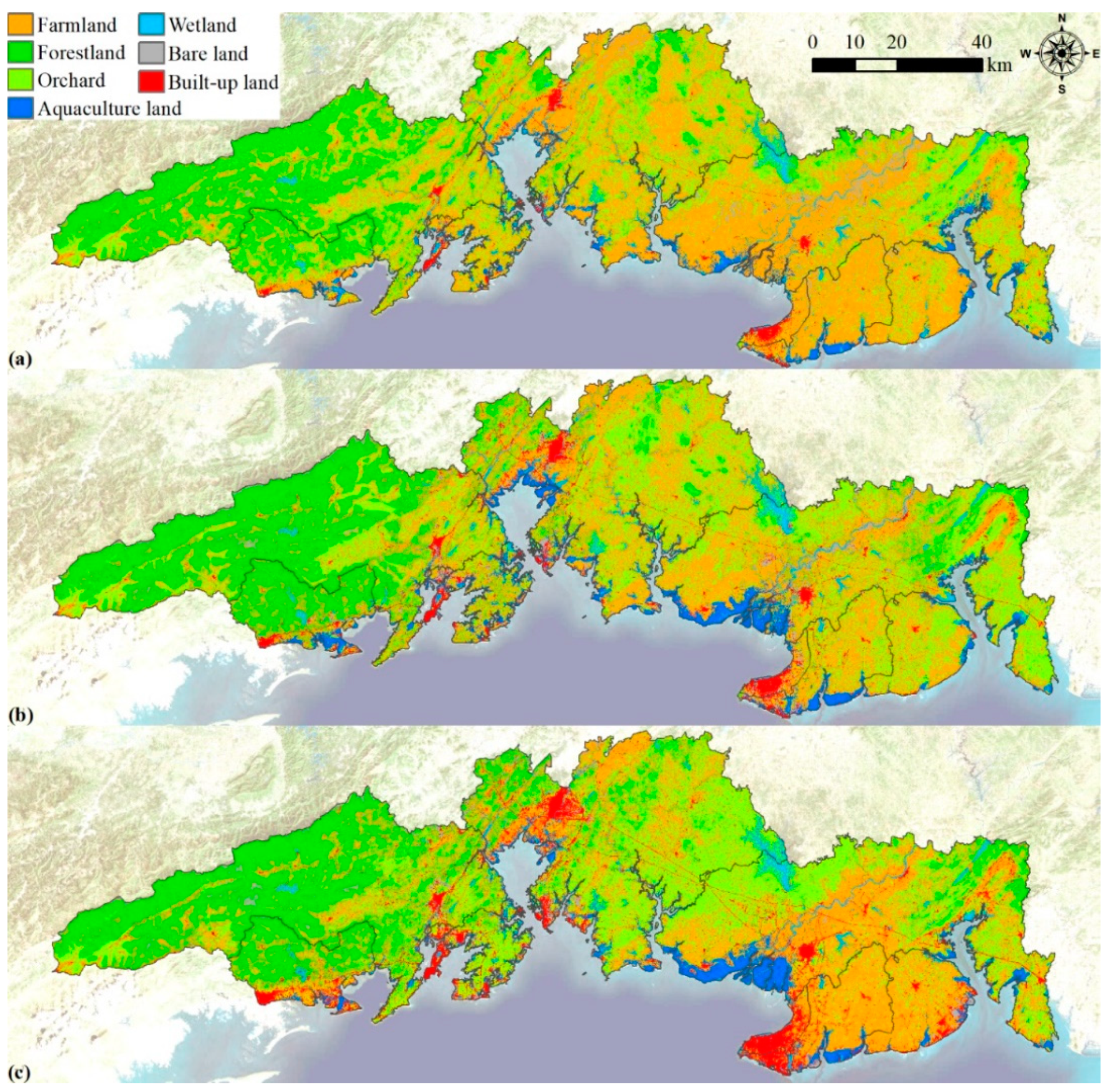
2.3.1. Land-Use Classification
2.3.2. Land-Use Change
- (1)
- Land-use structure information entropy
- (2)
- Land-use dynamic degree
- (3)
- Landscape pattern index
2.3.3. Hierarchical Clustering Analysis
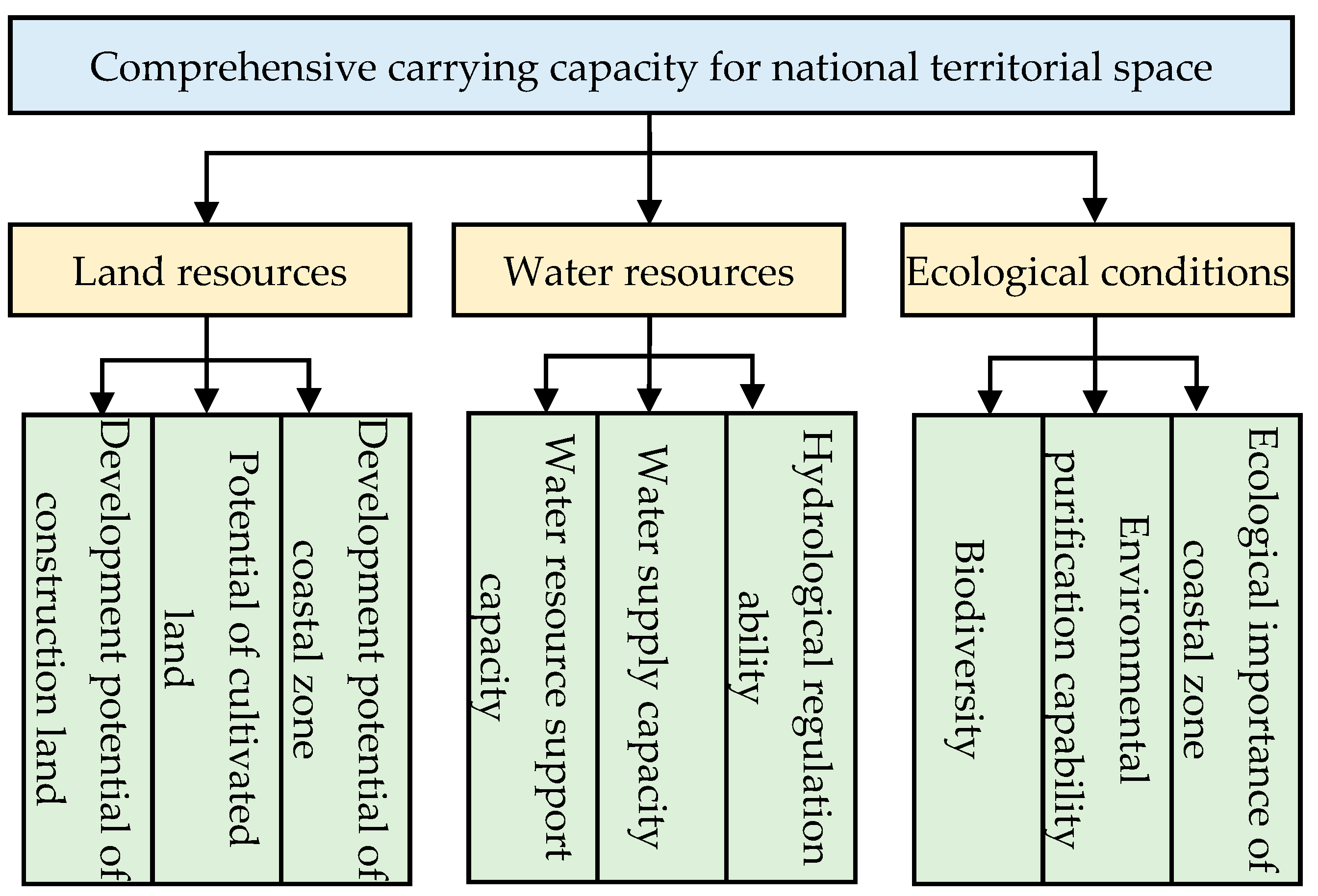
2.4. Comprehensive Carrying Capacity Evaluation
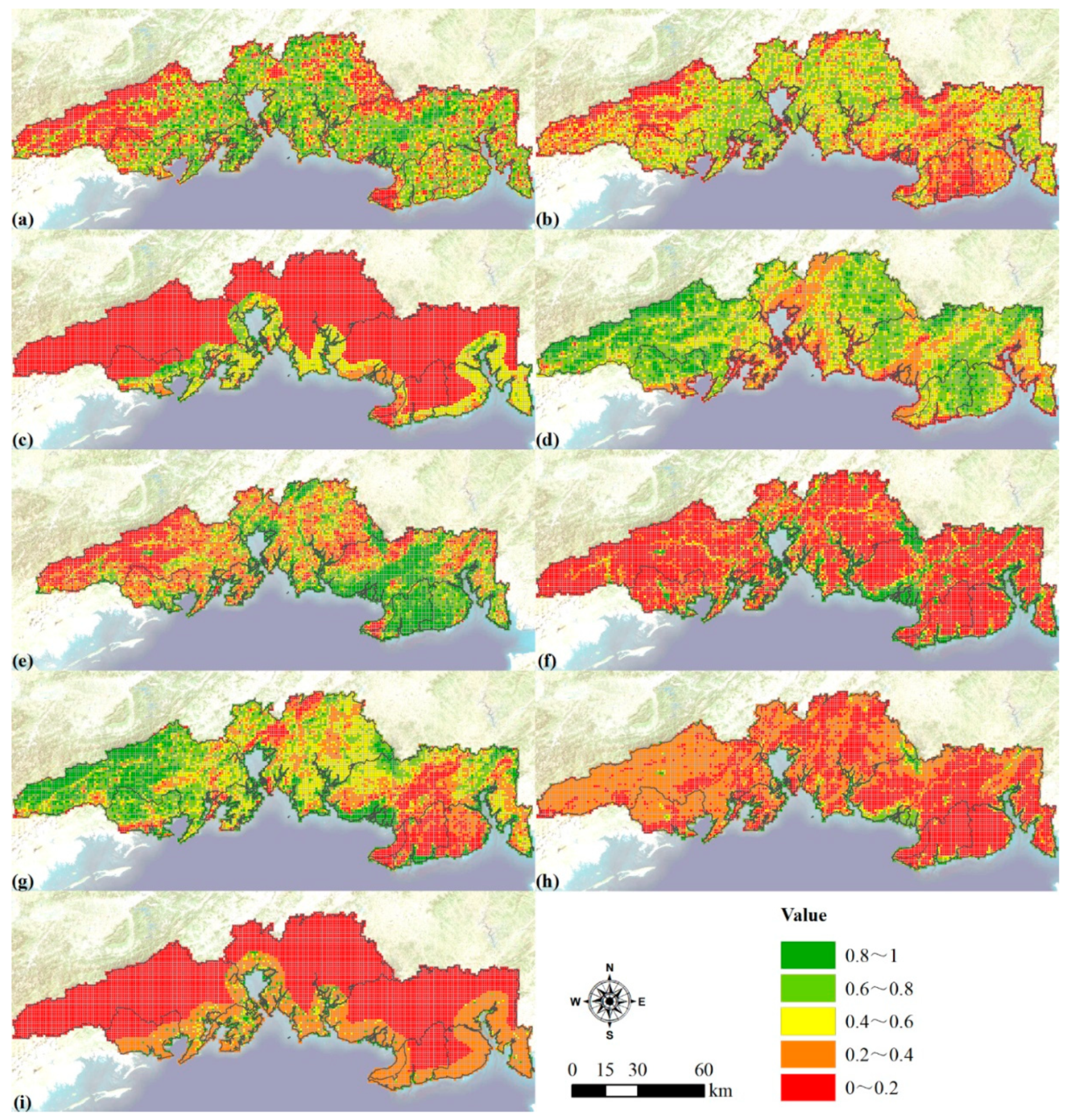
2.4.1. Carrying Capacity Index Calculation
- (1)
- Development potential of construction land
- (2)
- Potential of cultivated land
- (3)
- Development potential of coastal zone
- (4)
- Water resource support capacity
- (5)
- Water supply capacity
- (6)
- Hydrological regulation ability
- (7)
- Biodiversity
- (8)
- Environmental purification capability
- (9)
- Ecological importance of coastal zone
2.4.2. Weight of Carrying Capacity Index
3. Results
3.1. Land-Use Change
3.2. Spatial and Temporal Variation
3.3. Landscape Pattern Index Change
3.4. Carrying Capacity Index Evaluation
3.5. Comprehensive Carrying Capacity
4. Discussion
4.1. Dynamics of Territorial Spaces in the Past 20 Years
- (1)
- Land-use changes
- (2)
- Spatial and temporal variations
- (3)
- Landscape pattern index changes
4.2. Zoning Layout and Control Points Based on Comprehensive Carrying Capacity
- (1)
- Developed areas
- (2)
- Priority development areas
- (3)
- Ecological reserve areas
- (4)
- Coastal reserve areas
4.3. Limitations and Uncertainties
5. Conclusions
Author Contributions
Funding
Institutional Review Board Statement
Informed Consent Statement
Data Availability Statement
Conflicts of Interest
References
- Yılmaz, M.; Terzi, F. Measuring the patterns of urban spatial growth of coastal cities in developing countries by geospatial metrics. Land Use Policy 2021, 107, 105487. [Google Scholar] [CrossRef]
- Zhang, J.; Witkowski, A.; Tomczak, M.; Li, C.; McCartney, K.; Xia, Z.; Sponheimer, M. The sub-fossil diatom distribution in the Beibu Gulf (northwest South China Sea) and related environmental interpretation. PeerJ 2022, 10, e13115. [Google Scholar] [CrossRef] [PubMed]
- Luo, S.; Yan, W. Evolution and driving force analysis of ecosystem service values in Guangxi Beibu Gulf coastal areas, China. Acta Ecol. Sin. 2018, 38, 3248–3259. Available online: https://oversea.cnki.net/kns/detail/detail.aspx?FileName=STXB201809025&DbName=CJFQ2018 (accessed on 17 January 2021).
- Yu, G.; Liao, Y.; Liao, Y.; Zhao, W.; Chen, Q.; Kou, J.; Liu, X. Research on integrated coastal zone management based on remote sensing: A case study of Guangxi Beibu gulf. Reg. Stud. Mar. Sci. 2021, 44, 101710. [Google Scholar] [CrossRef]
- Zhao, D.; Xiao, M.; Huang, C.; Liang, Y.; Yang, Z. Land Use Scenario Simulation and Ecosystem Service Management for Different Regional Development Models of the Beibu Gulf Area. China. Remote Sens. 2021, 13, 3161. [Google Scholar] [CrossRef]
- Li, S.; Zhao, X.; Pu, J.; Miao, P.; Wang, Q.; Tan, K. Optimize and control territorial spatial functional areas to improve the ecological stability and total environment in karst areas of Southwest China. Land Use Policy 2021, 100, 104940. [Google Scholar] [CrossRef]
- Liu, P. Marine Ecological Construction and Economic Coordination in Beibu Gulf City Cluster of China. J. Coast. Res. 2020, 109, 19–26. [Google Scholar] [CrossRef]
- Du, P.; Hou, X.; Xu, H. Dynamic Expansion of Urban Land in China’s Coastal Zone since 2000. Remote Sens. 2022, 14, 916. [Google Scholar] [CrossRef]
- Long, C.; Dai, Z.; Wang, R.; Lou, Y.; Zhou, X.; Li, S.; Nie, Y. Dynamic changes in mangroves of the largest delta in northern Beibu Gulf, China: Reasons and causes. For. Ecol. Manag. 2022, 504, 119855. [Google Scholar] [CrossRef]
- Fu, B.; Zhang, L. Land-use change and ecosystem services:concepts, methods and progress. Prog. Geogr. 2014, 33, 441–446. Available online: https://oversea.cnki.net/kns/detail/detail.aspx?FileName=DLKJ201404001&DbName=CJFQ2014 (accessed on 17 January 2021).
- Castanho, R.A.; Naranjo Gómez, J.M.; Kurowska-Pysz, J. Assessing Land Use Changes in Polish Territories: Patterns, Directions and Socioeconomic Impacts on Territorial Management. Sustainability 2019, 11, 1354. [Google Scholar] [CrossRef] [Green Version]
- Qin, J.; Fu, R.; Nong, S.; Zheng, Y.; Yu, M.; Ma, Y.; Wen, J. Study on the Protection and Development of Ecological Barrier in Guangxi Beibu Gulf. For. Resour. Manag. 2011, 30. [Google Scholar] [CrossRef]
- Yu, D.; Hao, R. Research Progress and Prospect of Ecosystem Services. Adv. Earth Sci. 2020, 35, 804. Available online: https://oversea.cnki.net/kns/detail/detail.aspx?FileName=DXJZ202008003&DbName=CJFQ2020 (accessed on 17 January 2021).
- Li, K.; Feng, M.; Biswas, A. Driving factors and future prediction of land use and cover change based on satellite remote sensing data by the LCM model: A case study from Gansu province, China. Sensors 2020, 20, 2757. [Google Scholar] [CrossRef] [PubMed]
- Yang, Y.; Tian, Y.; Zhang, Q.; Tao, J.; Huang, Y.; Gao, C.; Lin, J.; Wang, D. Impact of current and future land use change on biodiversity in Nanliu River Basin, Beibu Gulf of South China. Ecol. Indic. 2022, 141, 109093. [Google Scholar] [CrossRef]
- Campbell, S. Green Cities, Growing Cities, Just Cities?: Urban Planning and the Contradictions of Sustainable Development. J. Am. Plan. Assoc. 1996, 62, 296–312. [Google Scholar] [CrossRef]
- Nasrollahi, Z.; Hashemi, M.; Bameri, S.; Mohamad Taghvaee, V. Environmental pollution, economic growth, population, industrialization, and technology in weak and strong sustainability: Using STIRPAT model. Environ. Dev. Sustain. 2020, 22, 1105–1122. [Google Scholar] [CrossRef]
- Zhang, M.; Gao, F.; Gao, J. The Coordination Effect of Marine and Land Resources Carrying Capacity of Coastal Areas in China. Proc. Bus. Econ. Stud. 2022, 5, 1–11. [Google Scholar] [CrossRef]
- Li, L. Tonkin Bay Rim Economic Sphere and China’s Five-Country Strategy. China Open. J. 2006, 1, 61165. [Google Scholar] [CrossRef]
- Mai, T.; Song, Z.; Liu, W. Economic spatial pattern of western region in China. Econ. Geogr. 2010, 30. [Google Scholar] [CrossRef]
- Ni, J.; Lin, J.; Ji, J.; Huang, D.; Yu, T.; Luo, F. Comprehensive risk assessment of marine radioactivity in the Beibu Gulf of Guangxi. Mar. Pollut. Bull. 2021, 172, 112795. [Google Scholar] [CrossRef] [PubMed]
- Zhang, Z.; Hu, B.; Qiu, H. Comprehensive assessment of ecological risk in southwest Guangxi-Beibu bay based on DPSIR model and OWA-GIS. Ecol. Indic. 2021, 132, 108334. [Google Scholar] [CrossRef]
- Zhou, W.; Yuan, G.; Luo, S. The Idea concerning Monitoring and Early Warning of Carrying Capacity of Resources and the Environment in Making Coordinated Development Plans for Land and Sea in Guangxi Zhuang Autonomous Region. Nat. Resour. Econ. Chin. 2015, 28, 8–12. Available online: https://oversea.cnki.net/kns/detail/detail.aspx?FileName=ZDKJ201510005&DbName=CJFQ2015 (accessed on 17 January 2021).
- Liu, Y.; Ye, G.; Han, S. Decoupling between industrial environmental pollution and industrial economic growth in Guangxi Beibu Gulf Economic Zone. IOP Conf. Ser. Earth Environ. Sci. 2020, 569, 12021. [Google Scholar] [CrossRef]
- Wen, C.; Liu, J. Review and Prospect of Coastal Zone Planning Based on Land and Sea Integration. Planners 2019, 35, 5–11. Available online: https://oversea.cnki.net/kns/detail/detail.aspx?FileName=GHSI201907003&DbName=CJFQ2019 (accessed on 17 January 2021).
- Liu, S.; Liao, Q.; Xiao, M.; Zhao, D.; Huang, C. Spatial and Temporal Variations of Habitat Quality and Its Response of Landscape Dynamic in the Three Gorges Reservoir Area, China. Int. J. Environ. Res. Public Health 2022, 19, 3594. [Google Scholar] [CrossRef]
- Liao, Q.; Wang, Z.; Huang, C. Green Infrastructure Offset the Negative Ecological Effects of Urbanization and Storing Water in the Three Gorges Reservoir Area, China. Int. J. Environ. Res. Public Health 2020, 17, 8077. [Google Scholar] [CrossRef]
- Zhao, D.; Xiao, M.; Huang, C.; Liang, Y.; An, Z. Landscape Dynamics Improved Recreation Service of the Three Gorges Reservoir Area, China. Int. J. Environ. Res. Public Health 2021, 18, 8356. [Google Scholar] [CrossRef]
- Wu, M.; Wu, J.; Zang, C. A comprehensive evaluation of the eco-carrying capacity and green economy in the Guangdong-Hong Kong-Macao Greater Bay Area, China. J. Clean. Prod. 2021, 281, 124945. [Google Scholar] [CrossRef]
- Wen, C.; Yang, G.; Wang, H. Integrated Indicator System of Eco -Tourism Environmental Load Capacit y in Nature Reserves. J. Agro-Environ. Sci. 2002, 4, 365–368. Available online: https://kns.cnki.net/kcms/detail/detail.aspx?FileName=NHBH200204023&DbName=CJFQ2002 (accessed on 17 January 2021).
- Xu, H. A Study on Information Extraction of Water Body with the Modified Normalized Difference Water Index (MNDWI). J. Remote Sens. 2005, 9, 589–595. Available online: https://oversea.cnki.net/kns/detail/detail.aspx?FileName=YGXB200505011&DbName=CJFQ2005 (accessed on 17 January 2021).
- Zhu, X.; Zhang, T. Evaluation of Comprehensive Carrying Capacity of Urban Agglomerations in Guangdong, Hong Kong and Macao Based on Entropy Method and Grey Correlation Method. J. Shanxi Norm. Univ. 2020, 34, 120–128. [Google Scholar] [CrossRef]
- Liu, R.; Pu, L.; Zhu, M.; Huang, S.; Jiang, Y. Coastal resource-environmental carrying capacity assessment: A comprehensive and trade-off analysis of the case study in Jiangsu coastal zone, eastern China. Ocean. Coast. Manage. 2020, 186, 105092. [Google Scholar] [CrossRef]
- Qiu, H.; Hu, B.; Zhang, Z. Impacts of land use change on ecosystem service value based on SDGs report--Taking Guangxi as an example. Ecol. Indic. 2021, 133, 108366. [Google Scholar] [CrossRef]
- Aplin, P.; Atkinson, P.M.; Curran, P.J. Fine Spatial Resolution Simulated Satellite Sensor Imagery for Land Cover Mapping in the United Kingdom. Remote Sens. Environ. 1999, 68, 206–216. [Google Scholar] [CrossRef]
- Harris, P.; Ventura, S. The integration of geographic data with remotely sensed imagery to improve classification in an urban area. Photogramm. Eng. Remote Sens. 1995, 61, 993–998. [Google Scholar]
- Chen, J.; Zhang, S.; Zheng, D. Uncertainty of the Quantitative Analysis on Landscape Patterns. Arid. Zone Res. 2005, 22, 63–67. [Google Scholar] [CrossRef]
- Li, X.; Bu, R.; Chang, Y.; Hu, Y.; Wen, Q.; Wang, X.; Xu, C.; Li, Y.; He, H. The response of landscape metrics against pattern scenarios. Acta Ecol. Sin. 2004, 24, 123–134. Available online: https://oversea.cnki.net/kns/detail/detail.aspx?FileName=STXB200401018&DbName=CJFQ2004 (accessed on 17 January 2021).
- Wang, Y.; Wang, Y.; Su, X.; Qi, L.; Liu, M. Evaluation of the comprehensive carrying capacity of interprovincial water resources in China and the spatial effect. J. Hydrol. 2019, 575, 794–809. [Google Scholar] [CrossRef]
- Feng, Z.; Sun, T.; Yang, Y.; Yan, H. The Progress of Resources and Environment Carrying Capacity: From Single-factor Carrying Capacity Research to Comprehensive Research. J. Resour. Ecol. 2018, 9, 125–134. [Google Scholar] [CrossRef]


| Territorial Space | Land-Use Type | Description |
|---|---|---|
| Production space | Farmland | Agricultural production land |
| Orchard | Fruit production land | |
| Aquaculture land | Aquaculture production land | |
| Ecological space | Forestland | Forests with the crown density more than 0.2 |
| Wetland | Oceans, rivers, lakes and mud flats | |
| Bare land | Abandoned land and bare rock | |
| Living space | Built-up land | Towns, roads and settlements |
| Territorial Space | Classification Examples in Satellite Images | |||
|---|---|---|---|---|
| Production space | 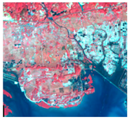 | 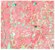 | 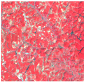 | 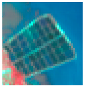 |
| Farmland (Paddy field) | Farmland (Dry land) | Orchard | Aquaculture land | |
| Ecological space | 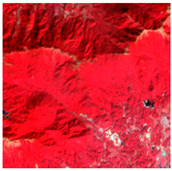 |  | 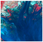 | 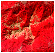 |
| Forestland | River | Lake | Bare rock | |
| Living space | 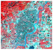 | 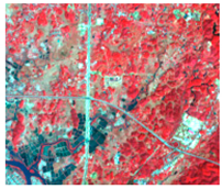 | ||
| Town and settlement | Road | |||
| Landscape Pattern Index | Study Scale | Significance |
|---|---|---|
| CA (Class Area) | Class scale | Describing the differences in patch distribution of different land-use types |
| NP (Number of Patches) | Class scale | Describing the number of patches of different land-use types and their degree of fragmentation |
| PD (Patch Density) | Class and landscape scales | Describing the fragmentation degree of patches of different land-use types for class scale, and the average fragmentation degree of all land-use patches in the entire study area for landscape scale |
| LPI (Largest Patch Index) | Class scale | Describing the dominant land-use type |
| PAFRC (Perimeter Area of Fractal Dimension) | Class scale | Describing the shape characteristics of patches of different land-use types |
| IJI (Interspersion and Juxtaposition Index) | Class scale | Describing the spatial distribution and juxtaposition of patches of different land-use types |
| LSI (Landscape Shape Index) | Landscape scale | Describing the comprehensive shape characteristics of patches of different land-use types throughout the study area |
| CONTAG (Contagion Index) | Landscape scale | Describing the extension trend of patches of different land-use types in the whole study area |
| COHESION (Cohesion index) | Landscape scale | Describing the degree of aggregation of patches of different land-use types throughout the study area |
| SHDI (Shannon’s Diversity Index) | Landscape scale | Describing each land-use type that tends to be distributed evenly throughout the study area |
| Target Layer | Criterion Layer | Weight | Indicator Layer | Weight |
|---|---|---|---|---|
| Comprehensive carrying capacity | Land resources | 0.399 | Development potential of construction land | 0.10374 |
| Potential of cultivated land | 0.08778 | |||
| Development potential of coastal zone | 0.20748 | |||
| Water resources | 0.229 | Water resources support capacity | 0.08015 | |
| Water supply capacity | 0.0916 | |||
| Hydrological regulation ability | 0.05725 | |||
| Ecological conditions | 0.372 | Biodiversity | 0.17856 | |
| Environmental purification capability | 0.08184 | |||
| Ecological importance of coastal zone | 0.1116 |
| Territorial Space | Land-Use Type | Land-Use Area (%) | Change Rate of Land-Use Area (%) | ||||
|---|---|---|---|---|---|---|---|
| 2000 | 2010 | 2020 | 2000–2010 | 2010–2020 | 2000–2020 | ||
| Production space | Farmland | 41.61 | 31.23 | 29.82 | −24.95 | −4.51 | −28.33 |
| Orchard | 28.88 | 30.82 | 30.76 | 6.7 | −0.18 | 6.51 | |
| Aquaculture land | 2.82 | 4.43 | 3.55 | 57.21 | −19.84 | 26.02 | |
| Ecological space | Forestland | 17.25 | 21.76 | 21.66 | 26.12 | −0.45 | 25.56 |
| Wetland | 3.28 | 3.39 | 4.12 | 3.08 | 21.74 | 25.5 | |
| Bare land | 3.86 | 4.27 | 3.19 | 10.65 | −25.29 | −17.34 | |
| Living space | Built-up land | 1.38 | 3.51 | 6.74 | 153.81 | 91.76 | 386.71 |
| Territorial Space | Land-Use Type | Land-Use Dynamic Degree (%) | ||
|---|---|---|---|---|
| 2000–2010 | 2010–2020 | 2000–2020 | ||
| Production space | Farmland | −3.56 | −0.56 | −1.89 |
| Orchard | 0.96 | −0.02 | 0.43 | |
| Aquaculture land | 8.17 | −2.48 | 1.73 | |
| Ecological space | Forestland | 3.73 | −0.06 | 1.7 |
| Wetland | 0.44 | 2.72 | 1.7 | |
| Bare land | 1.52 | −3.16 | −1.16 | |
| Living space | Built-up land | 21.97 | 11.47 | 25.78 |
| Territorial Space | Land-Use Type | Time | Landscape Pattern Index | |||||
|---|---|---|---|---|---|---|---|---|
| CA | NP | PD | LPI | PAFRAC | IJI | |||
| Production space | Farmland | 2000 | 368,541.18 | 47,276 | 2.34 | 4.77 | 1.48 | 55.29 |
| 2010 | 276,307.74 | 58,652 | 2.9 | 1.29 | 1.51 | 60.24 | ||
| 2020 | 264,707.73 | 55,799 | 2.76 | 3.08 | 1.47 | 65.5 | ||
| Orchard | 2000 | 255,871.71 | 73,713 | 3.64 | 1.07 | 1.49 | 49.86 | |
| 2010 | 273,161.07 | 65,598 | 3.24 | 1.08 | 1.49 | 49.07 | ||
| 2020 | 272,339.91 | 50,350 | 2.49 | 2.72 | 1.46 | 61.48 | ||
| Aquaculture land | 2000 | 32,269.5 | 9991 | 0.49 | 0.08 | 1.51 | 75.77 | |
| 2010 | 47,184.66 | 5822 | 0.29 | 0.62 | 1.48 | 90.26 | ||
| 2020 | 35,061.84 | 13,763 | 0.68 | 0.31 | 1.49 | 74.6 | ||
| Ecological space | Forestland | 2000 | 152,552.52 | 17,630 | 0.87 | 3.48 | 1.39 | 35.16 |
| 2010 | 192,423.33 | 30,192 | 1.49 | 6.42 | 1.45 | 54.39 | ||
| 2020 | 191,535.3 | 17,938 | 0.89 | 5.38 | 1.4 | 56.42 | ||
| Wetland | 2000 | 168,618.69 | 10,992 | 0.54 | 7.16 | 1.41 | 79.39 | |
| 2010 | 165,802.41 | 11,485 | 0.57 | 6.79 | 1.43 | 90.76 | ||
| 2020 | 171,593.19 | 22,319 | 1.1 | 2.87 | 1.43 | 90.92 | ||
| Bare land | 2000 | 34,228.71 | 45,739 | 2.26 | 0.01 | 1.45 | 44.91 | |
| 2010 | 38,382.57 | 37,661 | 1.86 | 0.02 | 1.36 | 66.4 | ||
| 2020 | 30,995.55 | 29,072 | 1.44 | 0.04 | 1.39 | 74.2 | ||
| Living space | Built-up land | 2000 | 12,466.44 | 8322 | 0.41 | 0.1 | 1.43 | 72.21 |
| 2010 | 32,659.29 | 25,807 | 1.27 | 0.19 | 1.44 | 80.2 | ||
| 2020 | 63,821.79 | 44,004 | 2.17 | 0.44 | 1.45 | 75.27 | ||
| Time | PD | LSI | CONTAG | COHESION | SHDI |
|---|---|---|---|---|---|
| 2000 | 11.69 | 216.46 | 46.14 | 99.60 | 1.62 |
| 2010 | 12.34 | 216.24 | 42.83 | 99.35 | 1.73 |
| 2020 | 11.77 | 191.17 | 43.40 | 99.31 | 1.73 |
| Zone | Main Function | Control Guidance |
|---|---|---|
| Developed areas | Production and living | No construction activities and maintaining current functions |
| Priority development areas | Industrial production and residential life | Urban construction and development |
| Agricultural production | Agriculture | |
| Fishery production | Aquaculture | |
| Port industry port construction | Port transportation | |
| Tourism | Modern service industry | |
| Ecological reserve areas | Environmental protection | Ecological protection, ecological restoration, controlled development and some consideration of ecological tourism |
| Coastal reserve areas | Ecological restoration | Mangrove restoration, coastal tourism |
Publisher’s Note: MDPI stays neutral with regard to jurisdictional claims in published maps and institutional affiliations. |
© 2022 by the authors. Licensee MDPI, Basel, Switzerland. This article is an open access article distributed under the terms and conditions of the Creative Commons Attribution (CC BY) license (https://creativecommons.org/licenses/by/4.0/).
Share and Cite
Ou, M.; Lai, X.; Gong, J. Territorial Pattern Evolution and Its Comprehensive Carrying Capacity Evaluation in the Coastal Area of Beibu Gulf, China. Int. J. Environ. Res. Public Health 2022, 19, 10469. https://doi.org/10.3390/ijerph191710469
Ou M, Lai X, Gong J. Territorial Pattern Evolution and Its Comprehensive Carrying Capacity Evaluation in the Coastal Area of Beibu Gulf, China. International Journal of Environmental Research and Public Health. 2022; 19(17):10469. https://doi.org/10.3390/ijerph191710469
Chicago/Turabian StyleOu, Menglin, Xiaochun Lai, and Jian Gong. 2022. "Territorial Pattern Evolution and Its Comprehensive Carrying Capacity Evaluation in the Coastal Area of Beibu Gulf, China" International Journal of Environmental Research and Public Health 19, no. 17: 10469. https://doi.org/10.3390/ijerph191710469
APA StyleOu, M., Lai, X., & Gong, J. (2022). Territorial Pattern Evolution and Its Comprehensive Carrying Capacity Evaluation in the Coastal Area of Beibu Gulf, China. International Journal of Environmental Research and Public Health, 19(17), 10469. https://doi.org/10.3390/ijerph191710469