
SANE (Easy Gait Analysis System): Towards an AI-Assisted Automatic Gait-Analysis


Abstract
:1. Introduction
1.1. AI for Pose Estimation
- PoseNet is an artificial intelligence programmed in Python using TensorFlow, a widely known machine learning framework created and maintained by Google. PoseNet recognizes 17 essential points: the eyes, ears, nose, shoulders, knees, hips, elbows, and ankles. PoseNet is capable of running on both CPUs and GPUs. This tool is available in two modes: a single-person pose detector that is quicker and easier to use but needs just one subject in the picture, and a multiple-person pose detector. One of the most compelling features of this skeleton tracking tool is its capacity to function nearly independently of the number of subjects evaluated concurrently [18].
- OpenPose is a free and open-source project. Currently, the framework supports two models: the COCO MPI model (which is quicker but less accurate) and the BODY 25 model. This skeleton tracking program is one of the few that can offer a greater and more comprehensive number of points, including critical spots on the feet and their angle [19].
- Nuitrack is a private closed-source application. It is a deep learning-based artificial intelligence. It is cross-platform, having capabilities for 3D full-body skeleton tracking, gesture recognition, and face tracking. Nuitrack detects 19 distinct points: it does not track the feet but does track the hands [20].
- Cubemos’ Skeleton Tracking SDK is a closed-source proprietary application that utilizes Intel’s Distribution of OpenVINO toolset. It is a machine learning-based artificial intelligence. It is a real-time, cross-platform, multi-person, 3D full-body posture estimator, although its use should be limited to scenes including up to five individuals. Cubemos recognizes the following 18 key points: eyes, ears, nose, shoulders, knees, wrists, hips, elbows, ankles, and spine. As a result, it is unable to offer information on the hands and feet or certain rotations. It is capable of using both CPUs and GPUs. Cubemos’ Skeleton Tracking SDK is optimized for use with Intel devices as an Intel partner [21].
1.2. General-Purpose Technologies for Motion Acquisition
- Non-optical:
- Instruments for magnetic, inertial, or electromechanical kinematic analysis. Electro-goniometers that detect 2D and 3D angular joint movement; accelerometers that compute up to six degrees of freedom of angular and linear joint movement.
- Pressure and dynamometric plates for dynamic analysis. Strain gauges or piezoelectric transducers are used to obtain information on the stresses and motions of the route [23].
- Electromyographic sensors for electromyographic analysis (EMG). They evaluate the action potentials of motor units and the neuromuscular activity responsible for movement [23].
- Optical:
- Passive markers are typically spherical or hemispherical in shape and coated with a retroreflective material to reflect light or a certain frequency.
- Active markers, on the other hand, are powered by a battery and incorporate an LED (generally producing infrared light, halving the distance it has to travel to be captured by cameras). However, they are double the size and expense of the passive alternative.
1.3. Gait-Analysis-Focused Technologies
2. Materials and Methods
2.1. Procedure
2.2. Description of the System
2.2.1. Tools
- The size
- 2.
- Sampling frequencies
- 3.
- Costs [40]
- 4.
- The ideal range of sampling distance
2.2.2. Front End
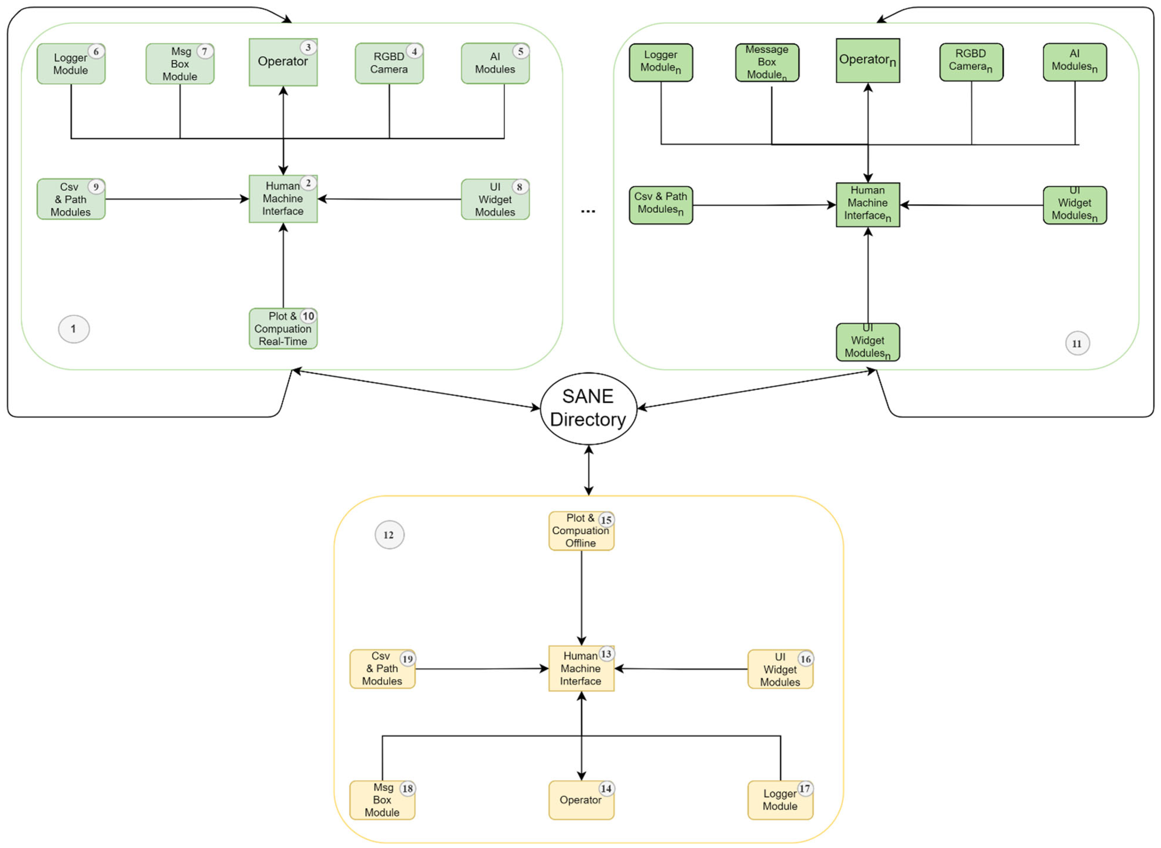
2.2.3. Back End
- The system behavior will be similar to the one reported in the following, independently of the hardware on which the SANE software is installed.
- The system performances will grow linearly and proportionally to the hardware specifics of the test setup.
- Two timestamps, one for the elapsed time between two consecutive frames and the other for the time elapsed from the beginning of the acquisition. Those are obtained by using a custom class derived from the built-in QTimer of PyQt.
- A list of the 3D skeleton key points in the considered frame.
- The processed image.
- 1.
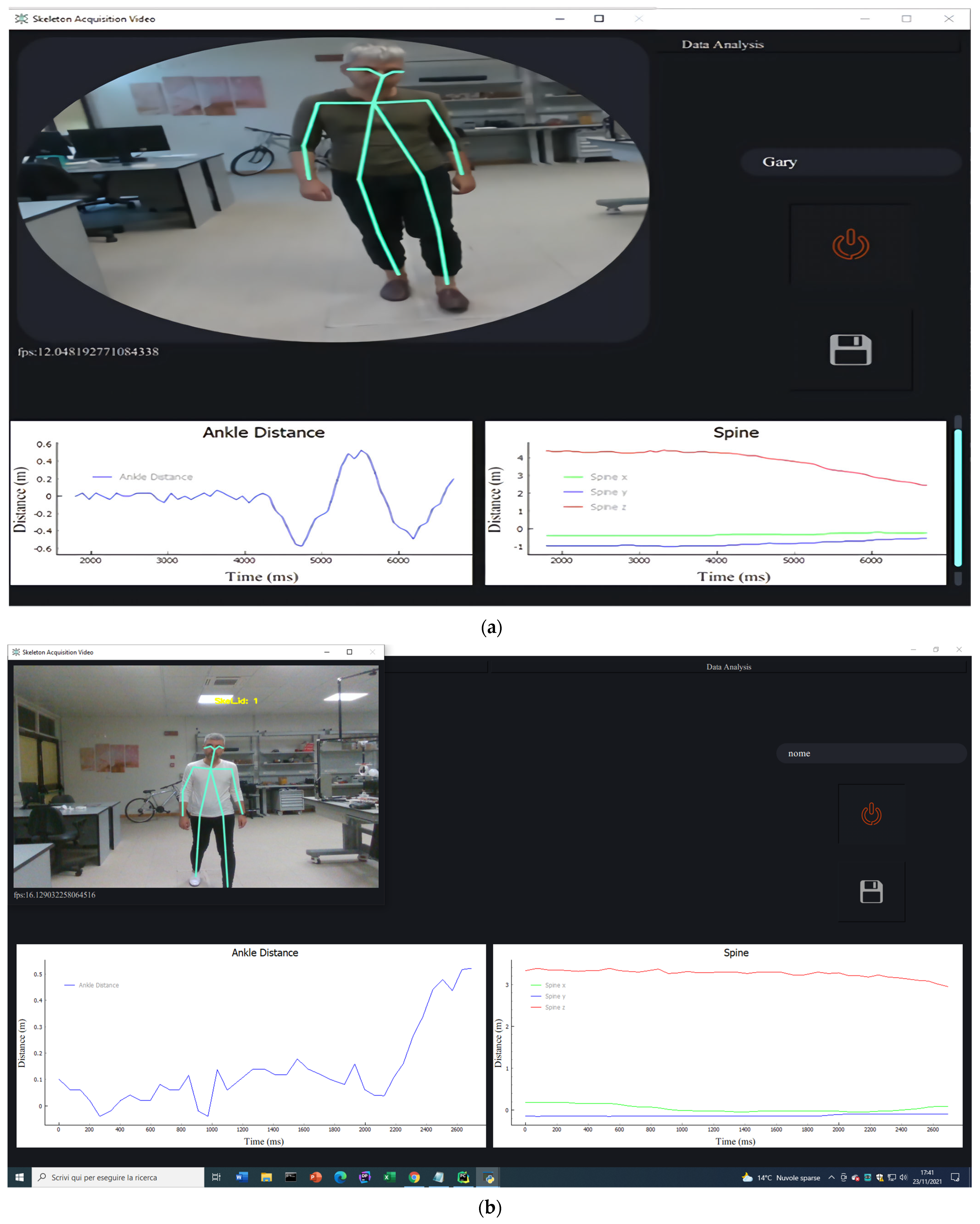
- The signal related to the “Pelvis” key point:It is computed as the midpoint between the “Right Hip” and “Left Hip” signals, is essential to compute several angles in gait analysis, and is a common reference point in motion tracking literature. Despite this, Cubemos does not provide this point, which is therefore computed at this moment. It consists of three further signals, which are the projection of the “Pelvis” on the X, the Y, and the Z axes.
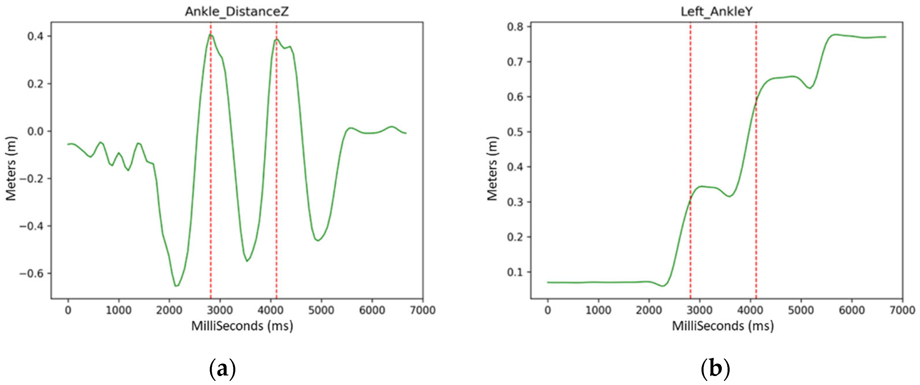
- 2.
- The “Ankle Distance” trend:It is a fundamental signal for gait recognition. It can be computed as the distance between the projection on the Z axis of the Left Ankle and the Right Ankle signals, specifically by subtraction of the former from the latter. Each time a gait cycle is performed, regardless of unsteadiness or asymmetry of the stride, the Ankle Distance signal has a sine-like shape with a complete period and with variable amplitude.
- 3.
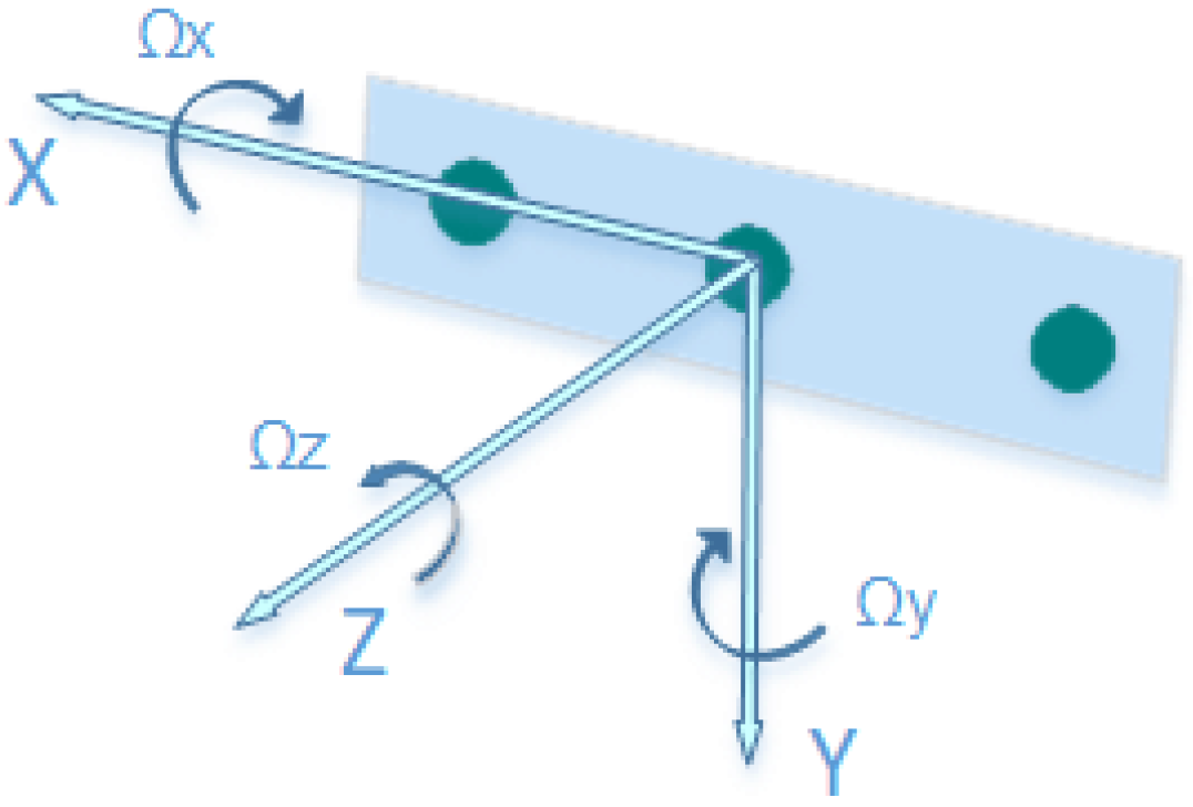
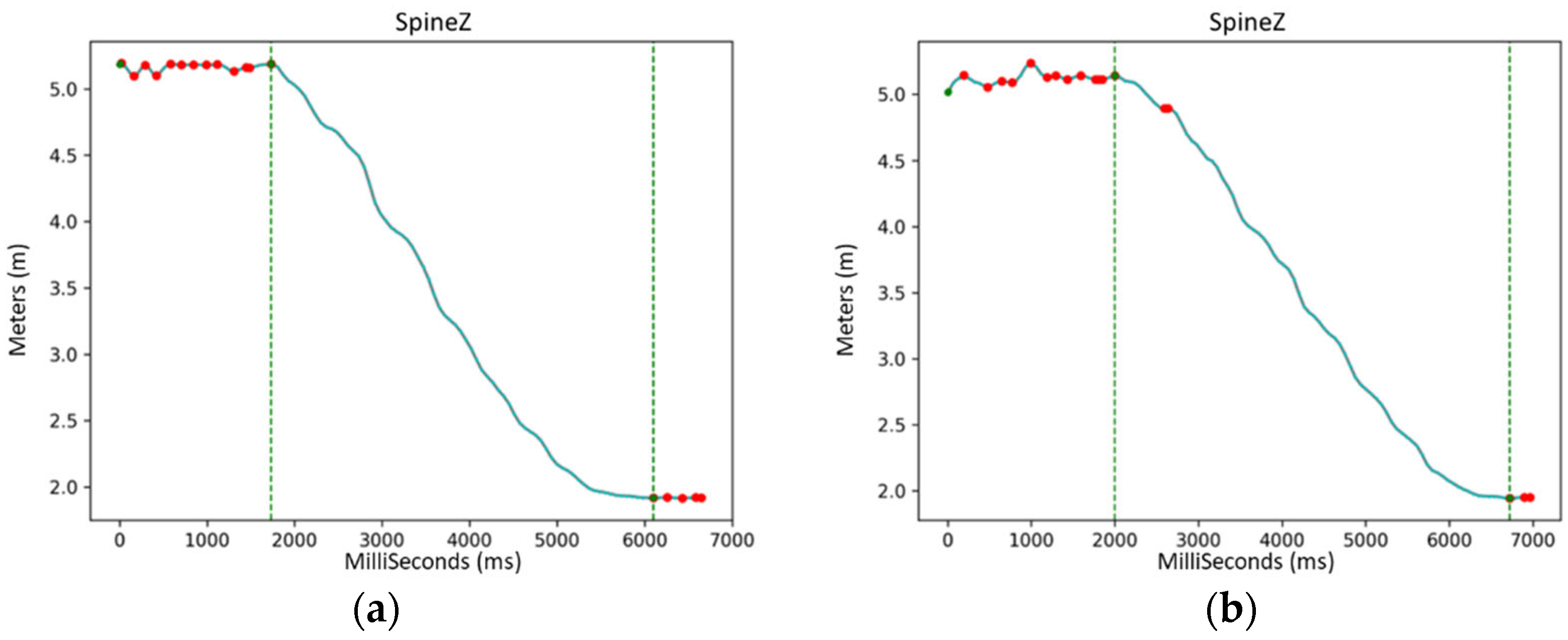
- The Total Displacement signal:It coincides with the range (R) defined by Intel RealSense, and it can be computed using Equation (2):where the addendums are the 3 dimensions of “Spine”, which is the key point commonly considered in the literature as the reference for the movement of the whole skeleton.
- 4.
- The FPS:It is computed as the reciprocal of the period between two frames, where standard numerical controls for real-time division must be employed.
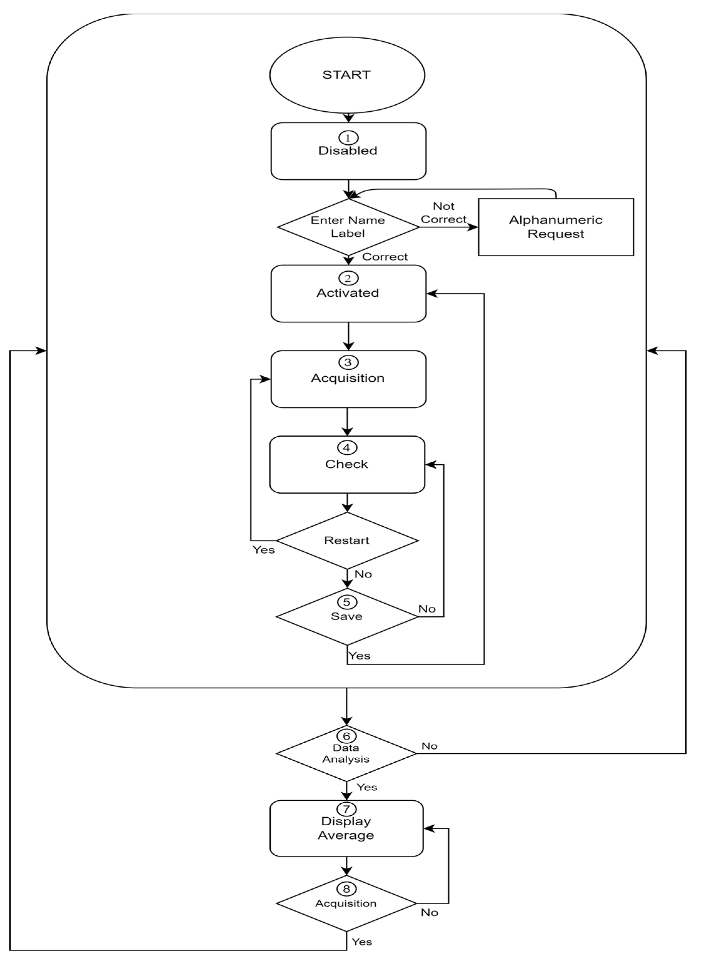
- The signal is not shaped in the form of a gait cycle: the number of steps is zero because the patient is not able to execute all the gait phases.
- The acquisition is non-continuous because the patient stopped moving during each cycle: the number of steps is zero since data are not suitable for analysis.
- The signal is not reliable either because too much noise is present in the video or because the AI outputs too many NaN results.
- The sampling time fell below the minimum 16 FPS threshold. This happens when the video is recorded on obsolete hardware or if the PC running SANE is executing too many programs simultaneously. Moreover, if some key points in every step have produced signals affected by noise, the operator receives a warning: the system is able to compute reliable averages provided that at least one of the acquisitions contains acceptable data of that signal. The operator is also warned if too much noise affects the acquisition.
- Scalar data such as speed, step duration and length, cadence, and cycle duration. These statistics are averaged over all the steps that are present in all the acquisitions of a single session.
- Kinematic data, specifically data about the variation in time of the angles associated with the step. These signals are averaged and normalized over all the steps that are present in all the acquisitions of a single session. The angles include obliquity, tilt, and rotation of the trunk; pelvic tilt and rotation; hip abduction/adduction and flexion/extension; the varus–valgus and flexion/extension of the knee. The signals for pelvic obliquity, knee and hip rotation, ankle dorsi-plantarflexion, and foot progression are not present since the points provided by Cubemos are not sufficient for mathematically defining these angles and recognizing body sections as the feet or the hands.
2.3. Statistical Analysis
- Inter-rater test: Two different operators perform the entire BTS marker placement procedure for the acquisition of two consecutive sessions, one each, of 10 walks, using SANE and BTS simultaneously on the same patient on the same day. The aim of these tests is not only to provide results from the two systems, but also to show the operator-induced measurement error between the two systems. In other words, it is an estimate of the systems’ dependency on the operator, as well as their reliability in this regard.
- In the context of this study, session 1 and session 2 were therefore associated with this test, performed by both operator 1 (Eval 1) and operator 2 (Eval 2)
- Test–retest: It is executed by the same operator who performs, on the same patient, on two consecutive days, two days apart [44], ex novo, the whole process for the placement of the markers predicted by the BTS to acquire two discontinuous and remote sessions of 10 walks using BTS and SANE concurrently. The aim of these tests is to demonstrate the difference between measurements collected in different periods by the same operator and patient. In other words, it is an evaluation of the systems’ dependence on time, as well as their reliability in this regard.
- In the context of this study, session 2 and session 3 were therefore associated with this test, performed by operator 2 (Eval 2).
- Intra-rater test: It is done by the same operator who performs, on the same patient on the same day, ex novo, the same process for the installation of the BTS-prescribed markers, for the acquisition of two consecutive sessions of 10 walks, using BTS and SANE concurrently. These tests are meant to demonstrate the variation between repeated measurements performed by the same operator on the same patient.
- In the context of this study, session 3 and session 4 were therefore associated with this test, performed by operator 2 (Eval 2).
3. Results
3.1. Gait Cycle Duration
3.2. Gait Step Duration
3.3. Gait Cadence
3.4. Gait Cycle Length
3.5. Gait Velocity
4. Discussion
5. Conclusions
Author Contributions
Funding
Institutional Review Board Statement
Informed Consent Statement
Data Availability Statement
Conflicts of Interest
References
- Somalvico, M. Intelligenza Artificiale. Scienza & Vita Nuova; Hewlett-Packard: Houston, TX, USA, 1987. (In Italian) [Google Scholar]
- Heaton, J. AIFH, Volume 3: Deep Learning and Neural Networks; Heaton Research, Inc.: Chesterfield, MI, USA, 2015. [Google Scholar]
- Lo-Ciganic, W.H.; Donohue, J.M.; Thorpe, J.M.; Perera, S.; Thorpe, C.T.; Marcum, Z.A.; Gellad, W.F. Using machine learning to examine medication adherence thresholds and risk of hospitalization. Med. Care 2015, 53, 720. [Google Scholar] [CrossRef] [PubMed]
- Alanazi, H.O.; Abdullah, A.H.; Qureshi, K.N.; Ismail, A.S. Accurate and dynamic predictive model for better prediction in medicine and healthcare. Ir. J. Med. Sci. 2018, 187, 501–513. [Google Scholar] [CrossRef]
- Musacchio, N.; Guaita, G.; Oz-zello, A.; Pellegrini, M.A.; Ponzani, P.; Zilich, R.; De Micheli, A. Intelligenza Artificiale e Big Data in ambito medico: Prospettive, opportunità, criticità. J. AMD 2018, 21, 3. [Google Scholar]
- Malva, A.; Zurlo, V. La medicina nell’era dell’Intelligenza Artificiale: Applicazioni in Medicina Generale. Dibatt. Sci. Prof. 2019, 26, 28. (In Italian) [Google Scholar]
- Annarumma, M.; Withey, S.J.; Bakewell, R.J.; Pesce, E.; Goh, V.; Montana, G. Automated triaging of adult chest radiographs with deep artificial neural networks. Radiology 2019, 291, 196–202. [Google Scholar] [CrossRef]
- Strodthoff, N.; Strodthoff, C. Detecting and interpreting myocardial infarction using fully convolutional neural networks. Physiol. Meas. 2019, 40, 015001. [Google Scholar] [CrossRef]
- Rajpurkar, P.; Hannun, A.Y.; Haghpanahi, M.; Bourn, C.; Ng, A.Y. Cardiologist-level arrhythmia detection with convolutional neural networks. arXiv 2017, arXiv:1707.01836. [Google Scholar]
- Madani, A.; Arnaout, R.; Mofrad, M.; Arnaout, R. Fast and accurate view classification of echocardiograms using deep learning. NPJ Digit. Med. 2018, 1, 6. [Google Scholar] [CrossRef]
- Zhang, J.; Gajjala, S.; Agrawal, P.; Tison, G.H.; Hallock, L.A.; Beussink-Nelson, L.; Deo, R.C. Fully automated echocardiogram interpretation in clinical practice: Feasibility and diagnostic accuracy. Circulation 2018, 138, 1623–1635. [Google Scholar] [CrossRef]
- Esteva, A.; Kuprel, B.; Novoa, R.A.; Ko, J.; Swetter, S.M.; Blau, H.M.; Thrun, S. Dermatologist-level classification of skin cancer with deep neural networks. Nature 2017, 542, 115–118. [Google Scholar] [CrossRef]
- Han, S.S.; Kim, M.S.; Lim, W.; Park, G.H.; Park, I.; Chang, S.E. Classification of the clinical images for benign and malignant cutaneous tumors using a deep learning algorithm. J. Investig. Dermatol. 2018, 138, 1529–1538. [Google Scholar] [CrossRef]
- Poria, S.; Majumder, N.; Mihalcea, R.; Hovy, E. Emotion recognition in conversation: Research challenges, datasets, and recent advances. IEEE Access 2019, 7, 100943–100953. [Google Scholar] [CrossRef]
- Eichstaedt, J.C.; Smith, R.J.; Merchant, R.M.; Ungar, L.H.; Crutchley, P.; Preoţiuc-Pietro, D.; Asch, D.A.; Schwartz, H.A. Facebook language predicts depression in medical records. Proc. Natl. Acad. Sci. USA 2018, 115, 11203–11208. [Google Scholar] [CrossRef]
- Reece, A.G.; Danforth, C.M. Instagram photos reveal predictive markers of depression. EPJ Data Sci. 2017, 6, 15. [Google Scholar] [CrossRef]
- Fitzpatrick, K.K.; Darcy, A.; Vierhile, M. Delivering cognitive behavior therapy to young adults with symptoms of depression and anxiety using a fully automated conversational agent (Woebot): A randomized controlled trial. JMIR Ment. Health 2017, 4, e7785. [Google Scholar] [CrossRef]
- Real-Time Human Pose Estimation in the Browser with Tensorflow.js. The TensorFlow Blog. Available online: https://blog.tensorflow.org/2018/05/real-time-human-pose-estimation-in.html (accessed on 19 October 2021).
- Demarchi, D.; Rabbito, R.; Bonato, P. Using Deep Learning-Based Pose Estimation Algorithms for Markerless Gait Analysis in Rehabilitation Medicine. Master’s Thesis, Polytechnic University of Turin, Turin, Italy, 2021. [Google Scholar]
- Nuitrack: Nuitrack.Skeleton Class Reference. Available online: https://download.3divi.com/Nuitrack/doc/classnuitrack_1_1Skeleton.html (accessed on 19 October 2021).
- Skeleton Tracking—SDK for Body Tracking Applications. Intel® RealSense™ Depth and Tracking Cameras. Available online: https://www.intelrealsense.com/skeleton-tracking/ (accessed on 19 October 2021).
- Baker, R. Gait analysis methods in rehabilitation. J. Neuroeng. Rehabil. 2006, 3, 4. [Google Scholar] [CrossRef]
- Muro-De-La-Herran, A.; Garcia-Zapirain, B.; Mendez-Zorrilla, A. Gait analysis methods: An overview of wearable and non-wearable systems, highlighting clinical applications. Sensors 2014, 14, 3362–3394. [Google Scholar] [CrossRef]
- Gomatam, A.N.M.; Sasi, S. Multimodal Gait Recognition Based on Stereo Vision and 3D Template Matching. In CISST; CSREA Press: Las Vegas, NV, USA, 2004; pp. 405–410. [Google Scholar]
- Liu, H.; Cao, Y.; Wang, Z. Automatic gait recognition from a distance. In Proceedings of the 2010 Chinese Control and Decision Conference, Xuzhou, China, 26–28 May 2010; pp. 2777–2782. [Google Scholar]
- Gabel, M.; Gilad-Bachrach, R.; Renshaw, E.; Schuster, A. Full body gait analysis with Kinect. In Proceedings of the 2012 Annual International Conference of the IEEE Engineering in Medicine and Biology Society, San Diego, CA, USA, 28 August–1 September 2012; pp. 1964–1967. [Google Scholar]
- Clark, R.A.; Pua, Y.H.; Bryant, A.L.; Hunt, M.A. Validity of the Microsoft Kinect for providing lateral trunk lean feedback during gait retraining. Gait Posture 2013, 38, 1064–1066. [Google Scholar] [CrossRef]
- Xue, Z.; Ming, D.; Song, W.; Wan, B.; Jin, S. Infrared gait recognition based on wavelet transform and support vector machine. Pattern Recognit. 2010, 43, 2904–2910. [Google Scholar] [CrossRef]
- M3D Force Plate (Wired)|Products|Tec Gihan Co., Ltd. Available online: https://www.tecgihan.co.jp/en/products/forceplate/small-for-shoes/m3d-force-plate-wired (accessed on 24 November 2021).
- Pirlo, G.; Luigi, M. Analisi Automatica del Gait in Malattie Neuro-Degenerative. Bachelor’s Thesis, University of Bari, Bari, Italy, 2018. [Google Scholar]
- Cutter, G.R.; Baier, M.L.; Rudick, R.A.; Cookfair, D.L.; Fischer, J.S.; Petkau, J.; Syndulko, K.; Weinshenker, B.G.; Antel, J.; Confavreux, C.; et al. Development of a multiple sclerosis functional composite as a clinical trial outcome measure. Brain 1999, 122, 871–882. [Google Scholar] [CrossRef]
- Hobart, J.C.; Riazi, A.; Lamping, D.L.; Fitzpatrick, R.; Thompson, A.J. Measuring the impact of MS on walking ability: The 12-Item MS Walking Scale (MSWS-12). Neurology 2003, 60, 31–36. [Google Scholar] [CrossRef]
- Holland, A.; O’Connor, R.J.; Thompson, A.J.; Playford, E.D.; Hobart, J.C. Talking the talk on walking the walk. J. Neurol. 2006, 253, 1594–1602. [Google Scholar] [CrossRef]
- Tinetti, M.E. Performance-oriented assessment of mobility problems in elderly patients. J. Am. Geriatr. Soc. 1986, 34, 119–126. [Google Scholar] [CrossRef]
- D’Amico, M.; Kinel, E.; D’Amico, G.; Roncoletta, P. A Self-Contained 3D Biomechanical Analysis Lab for Complete Automatic Spine and Full Skeleton Assessment of Posture, Gait and Run. Sensors 2021, 21, 3930. [Google Scholar] [CrossRef] [PubMed]
- Rosa, A.S.; Vargas, L.S.; Frizera, A.; Bastos, T. Real-Time Walker-Assisted Gait Analysis System Using Wearable Inertial Measurement Units. In Proceedings of the XXI Congresso Brasileiro de Automática—CBA2016, Vitoria, Brazil, 3–7 October 2016. [Google Scholar]
- Chaparro-Rico, B.D.M.; Cafolla, D. Test-Retest, Inter-Rater and Intra-Rater Reliability for Spatiotemporal Gait Parameters Using SANE (an eaSy gAit aNalysis systEm) as Measuring Instrument. Appl. Sci. 2020, 10, 5781. [Google Scholar] [CrossRef]
- New Technologies Group. Intel RealSense D400 Series Product Family Datasheet; Document Number: 337029-005; Intel Corporation: Santa Clara, CA, USA, 2019. [Google Scholar]
- Sipari, D. AI-Assisted Gait-Analysis: An Automatic and Teleoperated Approach. Master’s Dissertation, Politecnico di Torino, Turin, Italy, 2021. [Google Scholar]
- Intel RealSense Store. Intel® RealSenseTM Depth Camera D435i. Available online: https://store.intelrealsense.com/buy-intel-realsense-depthcamera-d435i.html (accessed on 24 November 2021).
- The Python Profilers—Python 3.10.0 Documentation. Available online: https://docs.python.org/3/library/profile.html#module-cProfile (accessed on 27 November 2021).
- Silva, L.M.; Stergiou, N. The basics of gait analysis. Biomech. Gait Anal. 2020, 164, 231. [Google Scholar]
- Krzysztof, M.; Mero, A. A kinematics analysis of three best 100 m performances ever. J. Hum. Kinet. 2013, 36, 149. [Google Scholar] [CrossRef]
- Marx, R.G.; Menezes, A.; Horovitz, L.; Jones, E.C.; Warren, R.F. A comparison of two time intervals for test-retest reliability of health status instruments. J. Clin. Epidemiol. 2003, 56, 730–735. [Google Scholar] [CrossRef]

| Method | Advantages | Disadvantages | Each Sensor Price (EUR) | Ref. | Accuracy |
|---|---|---|---|---|---|
| Camera Triangulation | High image resolution |
| 400 to 1900 | [24,25] | 70% [25] |
| No special conditions in terms of scene illumination | |||||
| Time of Flight | Only one camera is needed |
| 239 to 3700 | [23] | 2.66% to 9.25% (EER) [23] |
| It is not necessary to calculate depth manually | |||||
| Real-time 3D acquisition | |||||
| Reduced dependence on scene illumination | |||||
| Structured Light | Provides great detail |
| 160 to 200 | [26,27] | <1% (mean diff) [27] |
| Allows robust and precise acquisition of objects with arbitrary geometry and a wide range of materials | |||||
| Geometry and texture can be obtained with the same camera | |||||
| Infrared Thermography | Fast, reliable, and accurate output |
| 1000 to 18,440 | [28] | 78–91% |
| A large surface area can be scanned in no time | |||||
| Requires very little skill for monitoring |
| System | Advantages | Disadvantages |
|---|---|---|
| NWS |
|
|
| WS |
|
|
| First Day | Two Days Later | |
|---|---|---|
| Eval 1 | Session 1 | |
| Eval 2 | Session 2 | Session 3 Session 4 |
| SANE | BTS System | ||||
|---|---|---|---|---|---|
| Mean ± SD (s) | REM% | Mean ± SD (s) | REM% | ||
| Inter-rater relative error measurement | Session 1 | 1.33 ± 0.10 | 8.27 | 1.35 ± 0.11 | 7.41 |
| Session 2 | 1.44 ± 0.07 | 1.45 ± 0.04 | |||
| Test–retest relative error measurement | Session 2 | 1.44 ± 0.07 | 4.17 | 1.45 ± 0.04 | 4.83 |
| Session 3 | 1.38 ± 0.06 | 1.38 ± 0.04 | |||
| Intra-rater relative error measurement | Session 3 | 1.38 ± 0.06 | 1.45 | 1.38 ± 0.04 | 3.62 |
| Session 4 | 1.40 ± 0.06 | 1.43 ± 0.03 | |||
| SANE | BTS System | ||||
|---|---|---|---|---|---|
| Mean ± SD (s) | REM% | Mean ± SD (s) | REM% | ||
| Inter-rater relative error measurement | Session 1 | 0.66 ± 0.05 | 9.09 | 0.70 ± 0.12 | 22.86 |
| Session 2 | 0.72 ± 0.04 | 0.86 ± 0.02 | |||
| Test–retest relative error measurement | Session 2 | 0.72 ± 0.04 | 4.17 | 0.86 ± 0.02 | 5.81 |
| Session 3 | 0.69 ± 0.03 | 0.81 ± 0.02 | |||
| Intra-rater relative error measurement | Session 3 | 0.69 ± 0.03 | 1.45 | 0.81 ± 0.02 | 4.94 |
| Session 4 | 0.70 ± 0.03 | 0.85 ± 0.02 | |||
| SANE | BTS System | ||||
|---|---|---|---|---|---|
| Mean ± SD (Step/min) | REM% | Mean ± SD (Step/min) | REM% | ||
| Inter-rater relative error measurement | Session 1 | 91.48 ± 8.94 | 8.59 | 90.09 ± 5.24 | 8.09 |
| Session 2 | 83.62 ± 4.30 | 82.80 ± 2.29 | |||
| Test–retest relative error measurement | Session 2 | 83.62 ± 4.30 | 4.40 | 82.80 ± 2.29 | 5.51 |
| Session 3 | 87.30 ± 3.57 | 87.36 ±2.34 | |||
| Intra-rater relative error measurement | Session 3 | 87.30 ± 3.57 | 1.10 | 87.36 ±2.34 | 3.85 |
| Session 4 | 86.34 ± 3.98 | 84.00 ± 1.77 | |||
| SANE | BTS System | ||||
|---|---|---|---|---|---|
| Mean ± SD (m) | REM% | Mean ± SD (m) | REM% | ||
| Inter-rater relative error measurement | Session 1 | 1.40 ± 0.17 | 3.57 | 1.33 ± 0.16 | 1.50 |
| Session 2 | 1.45 ± 0.11 | 1.35 ± 0.04 | |||
| Test–retest relative error measurement | Session 2 | 1.45 ± 0.11 | 0.69 | 1.35 ± 0.04 | 5.93 |
| Session 3 | 1.46 ± 0.07 | 1.43 ± 0.03 | |||
| Intra-rater relative error measurement | Session 3 | 1.46 ± 0.07 | 2.74 | 1.43 ± 0.03 | 2.80 |
| Session 4 | 1.42 ± 0.08 | 1.39 ± 0.02 | |||
| SANE | BTS System | ||||
|---|---|---|---|---|---|
| Mean ± SD (m/s) | REM% | Mean ± SD (m/s) | REM% | ||
| Inter-rater relative error measurement | Session 1 | 1.05 ± 0.08 | 3.81 | 1.00± 0.10 | 10.00 |
| Session 2 | 1.01 ± 0.07 | 0.90 ± 0 | |||
| Test–retest relative error measurement | Session 2 | 1.01 ± 0.07 | 4.95 | 0.90 ± 0 | 11.11 |
| Session 3 | 1.06 ± 0.07 | 1.00 ± 0 | |||
| Intra-rater relative error measurement | Session 3 | 1.06 ± 0.07 | 3.77 | 1.00 ± 0 | 0.00 |
| Session 4 | 1.02 ± 0.06 | 1.00 ±0 | |||
Publisher’s Note: MDPI stays neutral with regard to jurisdictional claims in published maps and institutional affiliations. |
© 2022 by the authors. Licensee MDPI, Basel, Switzerland. This article is an open access article distributed under the terms and conditions of the Creative Commons Attribution (CC BY) license (https://creativecommons.org/licenses/by/4.0/).
Share and Cite
Sipari, D.; Chaparro-Rico, B.D.M.; Cafolla, D. SANE (Easy Gait Analysis System): Towards an AI-Assisted Automatic Gait-Analysis. Int. J. Environ. Res. Public Health 2022, 19, 10032. https://doi.org/10.3390/ijerph191610032
Sipari D, Chaparro-Rico BDM, Cafolla D. SANE (Easy Gait Analysis System): Towards an AI-Assisted Automatic Gait-Analysis. International Journal of Environmental Research and Public Health. 2022; 19(16):10032. https://doi.org/10.3390/ijerph191610032
Chicago/Turabian StyleSipari, Dario, Betsy D. M. Chaparro-Rico, and Daniele Cafolla. 2022. "SANE (Easy Gait Analysis System): Towards an AI-Assisted Automatic Gait-Analysis" International Journal of Environmental Research and Public Health 19, no. 16: 10032. https://doi.org/10.3390/ijerph191610032
APA StyleSipari, D., Chaparro-Rico, B. D. M., & Cafolla, D. (2022). SANE (Easy Gait Analysis System): Towards an AI-Assisted Automatic Gait-Analysis. International Journal of Environmental Research and Public Health, 19(16), 10032. https://doi.org/10.3390/ijerph191610032