Article

Emission Inventories and Particulate Matter Air Quality Modeling over the Pearl River Delta Region

1
Centre for Environmental and Marine Studies (CESAM), Department of Environment and Planning, University of Aveiro, 3810-193 Aveiro, Portugal
2
Department of Civil and Environmental Engineering, Faculty of Science and Technology, University of Macau, Macau, China
*
Author to whom correspondence should be addressed.
Int. J. Environ. Res. Public Health 2021, 18(8), 4155; https://doi.org/10.3390/ijerph18084155
Submission received: 1 February 2021 / Revised: 7 April 2021 / Accepted: 8 April 2021 / Published: 14 April 2021
(This article belongs to the Special Issue Air Pollution and Carbon Dioxide Emissions)

Abstract

:
The Pearl River Delta (PRD) region is located on the southeast coast of mainland China and it is an important economic hub. The high levels of particulate matter (PM) in the atmosphere, however, and poor visibility have become a complex environmental problem for the region. Air quality modeling systems are useful to understand the temporal and spatial distribution of air pollution, making use of atmospheric emission data as inputs. Over the years, several atmospheric emission inventories have been developed for the Asia region. The main purpose of this work is to evaluate the performance of the air quality modeling system for simulating PM concentrations over the PRD using three atmospheric emission inventories (i.e., EDGAR, REAS and MIX) during a winter and a summer period. In general, there is a tendency to underestimate PM levels, but results based on the EDGAR emission inventory show slightly better accuracy. However, improvements in the spatial and temporal disaggregation of emissions are still needed to properly represent PRD air quality. This study’s comparison of the three emission inventories’ data, as well as their PM simulating outcomes, generates recommendations for future improvements to atmospheric emission inventories and our understanding of air pollution problems in the PRD region.

1. Introduction

Particulate matter (PM) affects more people than any other air pollutant [1,2] and according to the World Health Organization (WHO) [3], the PM fractions relevant to human health are particles with an aerodynamic equivalent of a diameter less than or equal to 10 µm (PM10) and particles with an aerodynamic equivalent of a diameter less than or equal to 2.5 µm (PM2.5).
The Pearl River Delta (PRD) region is located in a transitional zone of the East Asian monsoon system. It comprises eleven municipalities; nine are located in mainland China (Guangdong province) and two in the Special Administrative Regions (SAR) of Hong Kong and Macau [4,5]. The PRD has become one of China’s three main economic hubs and it is one of the most densely urbanized regions in the world [6,7]. With rapid development in the region, PM concentration increases along with decreases in visibility have become critical problems [8]. The highest PM levels are observed in the winter months (i.e., December, January and February) when northerly winds bring air pollution from highly polluted areas to the region, and when lower mixing heights and smaller rainfall amounts and frequencies are registered. PM concentrations are lower in the summer months (i.e., June, July and August). In this season, southerly winds from the South China Sea, higher mixing height values and larger rainfall amounts and frequencies favor better air pollution dispersion and deposition [9,10,11].
Aiming to reduce the air pollution problems, the National Ambient Air Quality Standards (NAAQS) of China (GB 3095-2012) were updated by the Ministry of Environmental Protection, adding the PM2.5 annual and daily standards. The annual limit values of PM10 for special areas such as national parks (i.e., Grade-I standard) and others (i.e., Grade-II standard) were also reduced.
The last report on the progress of the prevention and control of air pollution in Chinese cities showed that air quality had improved when compared with previous years. The PRD registered the lowest concentration levels among all key regions in China (i.e., lower than the Yangtze River Delta and Beijing-Tianjin-Hebei). However, the region still does not fully comply with the NAAQS of China, mainly in the winter when coal-burning and meteorological conditions lead to frequent air pollution episodes [12].
Air quality modeling is a useful approach to better understanding atmospheric pollution patterns in the PRD region. Air pollution emissions are amongst the most important input data required for air quality modeling [13] and several atmospheric emission inventories are available that can be applied over the Asia region.
The Emissions Database for Global Atmospheric Research (EDGAR) is a global emission inventory developed by the European Commission and the Netherlands Environmental Assessment Agency. It provides gridded annual emissions with 0.1 degrees (≈10 km) of horizontal resolution. Anthropogenic emissions of greenhouse gases and air pollutants (namely PM10 and PM2.5) are calculated by applying a technology-based emission factor approach for domestic sources, road transport, industry and other sectors. Total national emissions by sector are spatially allocated using the location of manufacturing facilities, road networks, land use, and human and animal population densities [14].
The MIX Asia emission inventory was created using a combination of different regional atmospheric emission inventories [15,16,17,18,19,20], applying a mosaic approach. It includes monthly gridded emissions (at a 0.25-degree horizontal resolution) for the years 2008 and 2010 over Asia. These are aggregated into five activities: domestic, road transport, industry, power and agriculture. The emissions include gaseous pollutants, aerosols (i.e., PM10, PM2.5, organic carbon (OC) and black carbon (BC)), and speciated emissions for the SAPRC-99 (State Air Pollution Research Center 1999 version) and CB05 (Carbon Bond 5) chemical mechanisms [21]. Data on the locations of large emission sources, population densities, road networks and land use are used as spatial proxies to derive gridded emissions from each regional atmospheric emission inventory.
Kurokawa et al. [16] developed the Regional Emission inventory in Asia (REAS) emission inventory. It includes the major air pollutants (i.e., PM10 and PM2.5) and greenhouse gases over the Asia region. Monthly gridded emissions with a horizontal resolution of 0.25 × 0.25 degrees are provided for domestic sources, road transport, industry and other sectors. Atmospheric emissions are spatially disaggregated using population data, large point source locations, land cover data and road networks [16].
The main purpose of this work is to analyze the air quality modeling performance for PM10 and PM2.5 concentrations over the PRD, testing different atmospheric emission inventories. EDGAR, MIX and REAS are used to generate temporally and spatially disaggregated emissions as inputs for the air quality modeling system. The atmospheric emission inventories are tested in January (winter period) and July (summer period) of 2014 when the highest and lowest PM levels are recorded, respectively [10]. This year is selected based on its representativeness of the meteorological conditions that are generally observed over the study area and the availability of measured air quality data [10].
The paper is organized as follows. In Section 2, the air quality modeling setup and configuration are described. Section 3 presents and discusses the spatial and temporal disaggregation of the emission inventories. Section 4 concerns the system performance of the selected emission inventories. Finally, in Section 5, the main conclusions are presented.

2. Modeling Setup and Configuration

The air quality modeling system, composed of the Advanced Research Weather and Forecasting Model (WRF-ARW) [22] and the Comprehensive Air Quality Model with extensions (CAMx) [23] was used to simulate the air pollution levels over the PRD region. This air quality modeling system was selected since it has been extensively tested and shown to produce robust and realistic results [24,25,26]. Figure 1 shows the simulation domains used by the WRF-CAMx system and the cities/regions located over the innermost domain are identified.
The WRF-ARW (version 3.8) (National Center for Atmospheric Research, Boulder, CO, USA) [22] domains’ configuration consists of four nested grids: the larger domain comprises the major part of Asia with a grid spacing of 81 × 81 km2; the following domain, with a horizontal resolution of 27 × 27 km2, covers south-eastern China, the Korean Peninsula and part of south-eastern Asia; the last two domains cover the southeast coast of China and PRD region, with a horizontal resolution of 9 × 9 km2 and 3 × 3 km2, respectively. This model was initialized with global fields from the National Centre for Environmental Prediction, with a 1° by 1° spatial resolution and a temporal resolution of 6 h. The WRF-ARW input dataset provided information on topographies and land use/land cover data for each domain. The WRF-ARW for three different combinations of parameterization schemes for winter (i.e., January) and summer (i.e., July) was tested [27] and the following configuration was selected as the best set of parameterization schemes: the WRF Single-Moment 6-class scheme [28], the rapid radiative transfer model [29], Dudhia [30], the Monin-Obukhov similarity scheme [31,32,33], the Noah land surface model [34], the Kain-Fritsch scheme [35] and the Yonsei University scheme [36]. The same parameterization schemes were used for all WRF-ARW domains. For more information on the WRF evaluation performance for the PRD region during the simulation periods of this study (January and July), see Lopes et al. [27].
The CAMx (version 6.40) model (ENVIRON, Novato, CA, USA) simulates the atmospheric emissions, air pollution dispersion, chemical reactions and removal of pollutants in the troposphere by solving the Eulerian continuity equation for each chemical species in a system of nested three dimensional (3D) grids [23]. It is suitable for application to different scales ranging from global to sub-urban regions. In this study, the CAMx model was applied to two smaller WRF-ARW domains: a coarse domain covering the southeast coast of mainland China with 9 × 9 km2 of horizontal resolution (D1) and a nested domain comprising the PRD region with a grid spacing of 3 × 3 km2 (D2). Vertical and horizontal transport/advection were performed using the piecewise parabolic method and an implicit backward-Euler integration scheme [37]. Turbulent diffusion and chemistry were calculated using standard “K-theory” and an Euler backward iterative method, respectively. The surface ultraviolet albedo and surface resistance values for the dry deposition calculations, as well as the seasonal default surface roughness lengths and leaf area index values, were taken from the WESELY89 dry deposition option [23]. The Carbon Bond 6 (CB06) gas-phase mechanism was selected in this study. For PM, the CAMx aerosol scheme splits the particle size distribution into coarse and fine modes. Primary species are simulated as fine and/or coarse particles, while all chemically-formed compounds are modeled as fine particles only.
The global chemical MOZART model (National Center for Atmospheric Research, Colorado, United States of America) outputs every 6 h [38] were used to provide the initial and boundary conditions for the air quality model. Ozone column data were collected from the Total Ozone Mapping Spectrometer (TOMS) dataset [39]. The global inventory EDGAR [14], and the Asian inventories REAS [16] and MIX [21] were chosen to be tested with the air quality modeling system.

3. The Atmospheric Emission Inventories

This section presents the methodology used to generate temporally and spatially disaggregated emissions for the WRF-CAMx system. Results over the PRD study area from this disaggregation are also analyzed in more detail with further information regarding the total and spatial distributions of emissions.

3.1. Temporal and Spatial Disaggregation

To perform this work, data from the EDGAR, REAS and MIX emission inventories for the years 2008, 2008 and 2010, respectively, were used. The EDGAR, REAS and MIX emission inventories were adapted to generate temporal and spatial emissions for the WRF-CAMx domains. The daily profile for the domestic sector was based on the authors’ lived experiences in Chinese cities. Wang et al. [40] used the same methodology and obtained a similar temporal profile for the domestic sector. For road transport, temporal profiles were derived from the hourly variation of carbon monoxide (CO) concentrations at four roadside air quality monitoring stations (one in Macau SAR and three in Hong Kong SAR). These air quality data were obtained from the Macau Meteorological and Geophysical Bureau (SMG) and the Hong Kong Environmental Protection Bureau (HKEPD), respectively [41,42]. Li et al. [43] compared the CO concentrations measured at the roadside air quality monitoring station in the Macau SAR with the traffic volumes of several nearby roads. The results showed a high correlation between CO and road traffic volume, meaning that the temporal concentration variation of this pollutant could be used as the surrogate of the traffic volume. Zhang et al. [44] further recorded a similar temporal profile using mean hourly traffic counting during weekdays over the Macau SAR. For the other sectors, European temporal profiles were considered [45] due to the limited data available.
With the exceptions of the agricultural and international navigation sectors, the required resolution for the WRF-CAMx domain was obtained using land use and population data. Land use data with 500 m of horizontal resolution was provided by the United States Geological Survey Land Cover Institute [46]. For mainland China, the spatial population distribution developed by Fu et al. [47] with 1 × 1 km2 of horizontal resolution was used. For the Macau SAR, Hong SAR, Taiwan and the Philippines, a highly resolved spatial population distribution was produced using census [48,49,50,51] and land use datasets [46]. The population was only considered in the urban grids since the highest emissions and the largest numbers of inhabitants are observed in urban areas [52,53,54]. For the agricultural and international navigation sectors, a spatial disaggregation using only land use data was applied [46] and emissions were allocated to cropland grids and the ocean region, respectively.
The chosen chemical mechanism of the CAMx model requires the input of twenty-one gases and seven PM species including inert, organic and inorganic fractions (for detailed information, see [23]). A literature review was conducted and Chinese chemical speciation profiles were developed for road transport [55,56,57], domestic [58] and solvent activity sectors [59]. For the remaining sectors, the SPECIATE 4.4 database from the United States Environmental Protection Agency was used [60]. Taking into consideration that the EDGAR atmospheric emission inventory includes only annual emissions and the EDGAR and the REAS inventories have similar classifications of activities, the REAS inventory was used to create and apply to EDGAR a monthly temporal profile and a spatial speciation profile (by emission sector), over the CAMx modeling domains.

3.2. Total and Spatial Distribution Results

Based on the disaggregation methodology, PM emissions for the PRD study area were obtained. Figure 2 shows the PM (i.e., PM10 and PM2.5) emissions (kt) for each emission inventory by sector, in the winter (January) and summer (July) months, for the innermost WRF-CAMx domain (i.e., D2).
The EDGAR PM10 and PM2.5 emissions are higher than those from the other two inventories. This is mainly due to other sectors’ activities and domestic activities. For the other sectors, the reason for the large difference is the inclusion in the EDGAR inventory of more emission sources. The other sources in each inventory include the following emission activities: EDGAR) other transport, waste incineration, manure management, manufacturing and construction; MIX) this inventory does not include activities in this emission sector category; REAS) international navigation and other transport. For domestic sources, this is related to the approach used by EDGAR to spatially allocate the total national emissions. Because of the domestic sector’s contribution to the EDGAR inventory, it provides the highest total emissions during the winter when coal-burning is used for domestic heating. The industrial sector’s emissions are similar for the three emission inventories, with slightly higher values estimated by the REAS and MIX inventories. Moreover, the inventories also present similar total emissions for road transport, which is the smaller contributing sector. Besides, the atmospheric emissions provided by EDGAR, REAS and MIX are comparable with the values computed by other studies. For example, Zheng et al. [61] obtained PM10 and PM2.5 emissions of 687 kt (monthly average of about 57 kt) and 473 kt (monthly average of about 39 kt) for the year 2010 over Guangdong. This province includes Zhaoqing (not considered in this study), Guangzhou, Huizhou, Dongguan, Shenzhen, Zhuhai, Zhongshan and Foshan.
The spatial distributions of PM10 and PM2.5 during the winter and summer months are shown in Figure 3.
The EDGAR, MIX and REAS disaggregated data present the highest PM emissions in the north of Qingyuan (PM10 ≈ 300 t and PM2.5 ≈ 200 t), over the Macau peninsula (PM10 ≈ 70 t and PM2.5 ≈ 40 t) and Guangzhou (PM10 ≈ 50 t and PM2.5 ≈ 40 t), respectively (Figure 1 shows the locations). Focusing on the activity sectors with larger differences among the three inventories (i.e., domestic and other sectors), it is possible to identify for the domestic sector the highest emissions over different areas, for all inventories. For the other sectors, the EDGAR data show emissions mainly over the central region of the PRD (Guangzhou, Dongguan, Foshan and Zhongshan) while the REAS data result in similar values over the entire study area, including emissions over the South China Sea, which are due to international shipping activities. For road transport, emissions are higher over urban areas, and large industrial sector emissions values are estimated in Guangzhou for all of the tested inventories.
In the next section, the WRF-CAMx system’s performance for the winter and summer simulation months is presented using the EDGAR, MIX and REAS inventories.

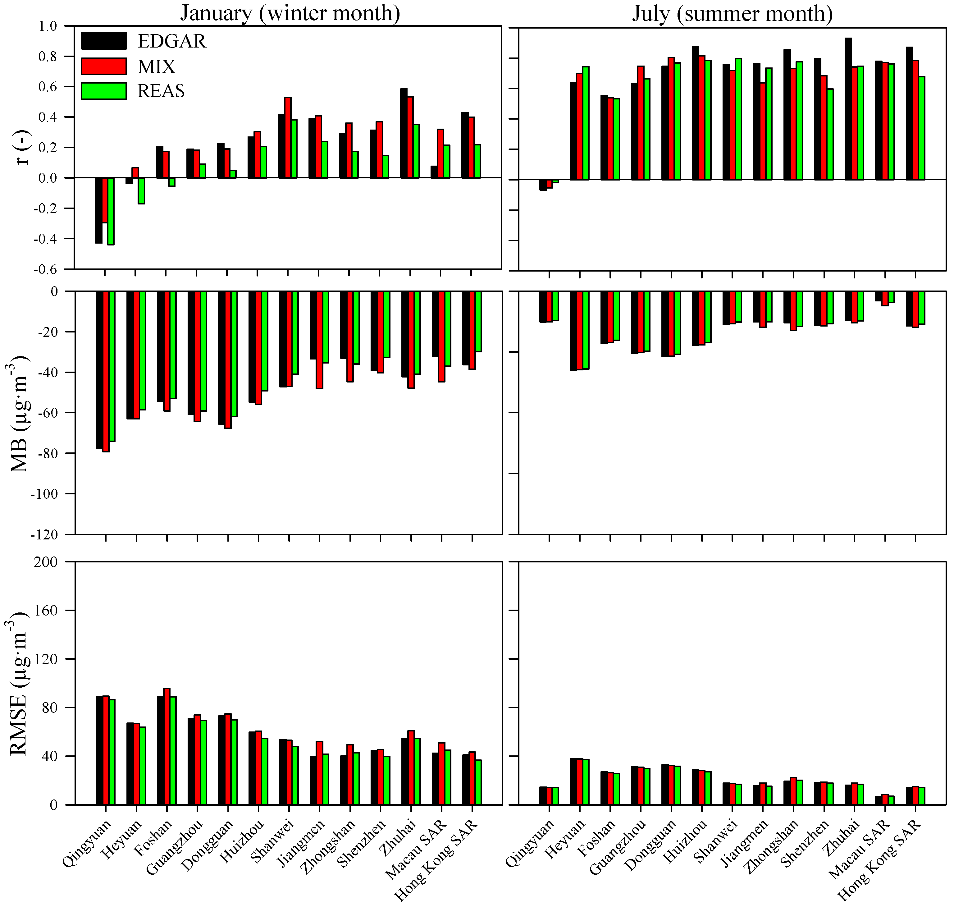
4. WRF-CAMx System Emissions Comparative Performance

The WRF-CAMx system was applied using the EDGAR, MIX and REAS inventories. The air quality modeling results were compared with data from thirteen air quality monitoring stations over the study region (one site for each city/region). An evaluation of the system’s performance for PM10 and PM2.5 was based on the methodologies proposed by Heinke and Sokhi [62] and Borrego et al. [63], and the following statistical parameters are presented: correlation coefficient (r), mean bias (MB) and root mean square error (RMSE). Figure 4 and Figure 5 depict comparative statistics between daily WRF-CAMx outputs and daily measured values of PM10 and PM2.5, respectively.
For PM10, the air quality modeling simulations revealed similar levels of accuracy using the different emission inventories. EDGAR-based results, however, showed a slightly better performance with higher correlation coefficients over the entire simulation domain and lower errors in the southern coastal regions of mainland China. Higher correlations and lower errors were obtained for the summer month when lower air pollution concentrations over the simulation domain were measured. The correlation coefficient ranged from −0.41 to 0.46 (REAS and MIX) in the winter month and 0.08 to 0.93 (REAS and EDGAR) in the summer month. These results are in agreement with previous studies, for example, a correlation coefficient of 0.32 (hourly model performance evaluation) for a summer episode was obtained by [64] for a modeling simulation over the PRD region. [65] calculated a correlation coefficient of 0.47 and 0.57 (daily model performance evaluation) for a winter and summer period, respectively. The current simulations tended to underestimate the PM10 levels (negative MB and time series are presented in Figure 6) for both seasons, which is a common behavior for PM10 simulations over the study region (e.g., [65,66]). The overestimation of wind speed by the WRF-CAMx system [27] may have contributed to the dispersion of atmospheric pollutants, leading to lower PM10 concentrations [67]. The magnitudes of errors ranged from 62.7 to 168 µg·m−3 (EDGAR and MIX) in January and 15·8 to 63·5 µg·m−3 (EDGAR) in July. These results are in agreement with those obtained by Xun-lai et al. [64] during an autumn episode (RMSE was 36 µg·m−3).
Similar to the PM10 results, the WRF-CAMx outputs with the EDGAR emission inventory showed a slightly better accuracy for PM2.5 simulations, as well (Figure 5). The best PM2.5 performance (higher correlation coefficient and lower error) was also found in the summer period. Qin et al. [65] and Kwok et al. [66] observed the same behavior for PM2.5 simulations over the study region. The correlation coefficient ranged from −0.44 to 0.58 (REAS and EDGAR) for the winter month and −0.07 to 0.93 (EDGAR and EDGAR) for the summer month. These daily results are similar to those obtained by Qin et al. [65] in the winter (r = 0.60) and summer (r = 0.87), but the results of this work were less satisfactory than those presented by Liu et al. [68], with a correlation coefficient ranging from 0.74 to 0.94. However, these authors obtained this air quality modeling performance for a shorter air pollution episode (24 h). The modeling system tends, as observed for PM10, to underestimate the PM2.5 levels (negative MB and time series are presented in Figure 6) for both seasons. The RMSE varied from 36.7 to 95.6 µg·m−3 (REAS and MIX) and 6.87 to 38.0 µg·m−3 (EDGAR) in winter and summer, respectively. Wang et al. [69] obtained an RMSE of 28 µg·m−3 in winter and 10 µg·m−3 in summer, while Chen et al. [26] recorded an RMSE of 21.75 µg·m−3 in winter. Besides, Liu et al. [68] computed an RMSE of between 29.0 and 56.5 µg·m−3 for an air pollution episode (24 h) over the PRD.
Figure 6 provides the time series for January and July at four air quality monitoring stations located near the main PM sources (Guangzhou) and the coastline (Zhuhai, Macau SAR and Hong Kong SAR).
Despite an underestimation, globally, WRF-CAMx when using different atmospheric emission inventories presents similar results, and the inventories can capture air pollution’s seasonality (with the highest levels in January and the lowest in July). In the winter season, domestic coal-burning leads to frequent air pollution episodes [12], which are not properly captured by the simulation because this air pollution source over the PRD region is underestimated [66]. In the summer period, the system’s ability to simulate the observed magnitude peaks is lower under the predominant typhoons and Pacific high system weather conditions [70,71]. In the particular simulated 2014 summer month, air pollution episodes were measured by almost all air quality monitoring stations on 7–9 and 21–23 July. In these periods, the region was affected by the approach of typhoons [41]. The air pollution episodes were recorded three days before each typhoon landed. These results are in agreement with previous studies over the Southeast Asian region where, before the arrival of a typhoon, high air pollution levels are observed at the periphery of the typhoon’s affected area due to the impact of downdrafts, atmospheric circulation field distribution and a high/uniform pressure system at the tropical cyclone front [70,72,73]. Under these conditions, it is difficult to obtain good simulation results, whatever emission inventory is used.
Figure 7 and Figure 8 display the spatial distributions of modeled monthly average concentrations of PM10 and PM2.5, respectively, for the winter (January) and summer months (July) using the EDGAR, MIX and REAS emission inventories. Measured monthly averages for the air quality monitoring stations are also represented by small circles.
Air quality modeling results, when applying EDGAR, REAS or MIX, show different spatial distributions of PM levels, but high values for all tested study cases are estimated over the Guangzhou region. The inventories reproduce reasonably well the air pollution concentrations over the study area in summer but they are less satisfactory in winter. These results may be due to uncertainties in the atmospheric emission inventories, namely the poor representation of local sources’ characteristics and locations or spatial variability of emission values, along with errors in the meteorological simulations related to particular weather events.

5. Conclusions

This work aimed to evaluate the WRF-CAMx system’s performance when simulating PM10 and PM2.5 concentrations over the PRD region using different atmospheric emission inventories (i.e., EDGAR, MIX and REAS). In general, the EDGAR, MIX and REAS emission inventories presented higher atmospheric emissions in the winter than in the summer period. The major differences between them were obtained for the domestic and other sectors. For all remaining activities, the total values and spatial distributions of emissions were similar among the three emission inventories. The PM simulation results with EDGAR showed a slightly better performance. The quality of the results is comparable to other air quality modeling applications over the study region, with an underestimation of PM levels. The system still requires improvements in the atmospheric emission inventories’ disaggregation, focusing on the temporal and spatial distributions of local air emission sources and on the contribution of natural sources, such as wildfires and sea salt biogenic emissions, as well as road dust resuspension.
These results could help to improve atmospheric emissions’ estimation and our understanding of air pollution problems over the PRD region.

Author Contributions

Software, D.L. and J.F.; visualization, D.L.; writing—original draft, D.L., J.F. and K.I.H.; formal analysis, K.-V.Y.; funding acquisition, K.M.M. and A.I.M.; writing—review and editing, K.M.M. and A.I.M. All authors have read and agreed to the published version of the manuscript.

Funding

This study was supported by the Science and Technology Development Fund of the Macau SAR government under grant No. 079/2013/A3, as well as the university multi-year research grant (MYRG-2014-00038-FST) of the research committee of the University of Macau, and the university’s postgraduate studentship. This work was performed in part at the High-Performance Computing Cluster (HPCC), which is supported by the Information and Communication Technology Office (ICTO) of the University of Macau. J.F. is funded by national funds (OE), through FCT (Fundação para a Ciência e Tecnologia), in the scope of the framework contract foreseen in numbers 4, 5 and 6 of article 23 of the Decree-Law 57/2016, of 29 August, changed by Law 57/2017, of 19 July. Thanks are also due for the financial support of Centre for Environmental and Marine Studies (CESAM) (UIDB/50017/2020 + UIDP/50017/2020), to FCT/MCTES (Fundação para a Ciência e Tecnologia/Ministério da Ciência, Tecnologia e Ensino Superior) for national funds, and for co-funding from the FEDER (Fundo Europeu de Desenvolvimento Regional), within the PT2020 Partnership Agreement and Compete 2020.

Institutional Review Board Statement

Not applicable.

Informed Consent Statement

Not applicable.

Conflicts of Interest

The authors declare no conflict of interest. The funders played no role in the design of the study; in the collection, analyses, or interpretation of the data; in writing the manuscript; or in the decision to publish the results.

References

  1. WHO (World Health Organization). Ambient (Outdoor) Air Quality and Health. Available online: http://www.who.int (accessed on 31 January 2021).
  2. Costa, S.; Ferreira, J.; Silveira, C.; Costa, C.; Lopes, D.; Relvas, H.; Borrego, C.; Roebeling, P.; Miranda, A.I.; Paulo Teixeira, J. Integrating Health on Air Quality Assessment—Review Report on Health Risks of Two Major European Outdoor Air Pollutants: PM and NO2. J. Toxicol. Environ. Health Part B Crit. Rev. 2014, 17, 307–340. [Google Scholar] [CrossRef]
  3. WHO (World Health Organization). Health Effects of Particulate Matter: Policy Implications for Countries in Eastern Europe, Caucasus and Central Asia; World Health Organization Regional Office for Europe: Copenhagen, Denmark, 2013; Volume 50. [Google Scholar]
  4. Bie, J.; De Jong, M.; Derudder, B. Greater Pearl River Delta: Historical Evolution towards a Global City-Region. J. Urban Technol. 2015, 22, 103–123. [Google Scholar] [CrossRef]
  5. Huang, H.; Ho, K.F.; Lee, S.C.; Tsang, P.K.; Ho, S.S.H.; Zou, C.W.; Zou, S.C.; Cao, J.J.; Xu, H.M. Characteristics of carbonaceous aerosol in PM2.5: Pearl Delta River Region, China. Atmos. Res. 2012, 104–105, 227–236. [Google Scholar] [CrossRef]
  6. Zhao, S.X.B.; Zhang, L. Foreign Direct Investment and the Formation of Global City-Regions in China. Reg. Stud. 2007, 41, 979–994. [Google Scholar] [CrossRef]
  7. Florida, R.; Gulden, T.; Mellander, C. The rise of the mega-region. Camb. J. Reg. Econ. Soc. 2008, 1, 459–476. [Google Scholar] [CrossRef]
  8. Chen, J.; Xin, J.; An, J.; Wang, Y.; Liu, Z.; Chao, N.; Meng, Z. Observation of aerosol optical properties and particulate pollution at background station in the Pearl River Delta region. Atmos. Res. 2014, 143, 216–227. [Google Scholar] [CrossRef]
  9. Hoi, K.I.; Mok, K.M.; Yuen, K.V.; Pun, M.H. Investigation of fine particulate pollution in a coastal city with a mobile monitoring platform. Glob. NEST J. 2013, 15, 178–187. [Google Scholar] [CrossRef]
  10. Lopes, D.; Hoi, K.I.; Mok, K.M.; Miranda, A.I.; Yuen, K.V.; Borrego, C. Air quality in the main cities of the Pearl River Delta region. Glob. Nest J. 2016, 18, 794–802. [Google Scholar] [CrossRef]
  11. Mok, K.M.; Hoi, K.I. Effects of meteorological conditions on PM10 concentrations—A study in Macau. Environ. Monit. Assess. 2005, 102, 201–223. [Google Scholar] [CrossRef] [PubMed]
  12. CAA (Clean Air Asia). Air Pollution Prevention and Control Progress in Chinese Cities; CAA: Beijing, China, 2016. [Google Scholar]
  13. Ferreira, J.; Lopes, D.; Rafael, S.; Relvas, H.; Almeida, S.M.; Miranda, A.I. Modelling air quality levels of regulated metals: Limitations and challenges. Environ. Sci. Pollut. Res. 2020, 27, 33916–33928. [Google Scholar] [CrossRef]
  14. EC-JRC/PBL. Emission Database for Global Atmospheric Research Version 4.2. Available online: https://data.jrc.ec.europa.eu/collection/edgar (accessed on 1 October 2015).
  15. MEIC (Multi-Resolution Emission Inventory for China). Available online: http://www.meicmodel.org (accessed on 12 June 2017).
  16. Kurokawa, J.; Ohara, T.; Morikawa, T.; Hanayama, S.; Janssens-Maenhout, G.; Fukui, T.; Kawashima, K.; Akimoto, H. Emissions of air pollutants and greenhouse gases over Asian regions during 2000-2008: Regional Emission inventory in ASia (REAS) version 2. Atmos. Chem. Phys. 2013, 13, 11019–11058. [Google Scholar] [CrossRef] [Green Version]
  17. Hung, X.; Song, Y.; Li, M.; Li, J.; Huo, Q.; Cai, X.; Zhu, T.; Hu, M.; Zhang, H. A high-resolution ammonia emission inventory in China. Glob. Biogeochem. Cycles 2012, 26. [Google Scholar] [CrossRef]
  18. Lu, Z.; Zhang, Q.; Streets, D.G. Sulfur dioxide and primary carbonaceous aerosol emissions in China and India, 1996–2010. Atmos. Chem. Phys. 2011, 11, 9839–9864. [Google Scholar] [CrossRef] [Green Version]
  19. Lu, Z.; Streets, D.G. Increase in NOx emissions from indian thermal power plants during 1996–2010: Unit-based inventories and multisatellite observations. Environ. Sci. Technol. 2012, 46, 7463–7470. [Google Scholar] [CrossRef] [PubMed]
  20. Lee, D.-G.; Lee, Y.-M.; Jang, K.; Yoo, C.; Kang, K.; Lee, J.-H.; Jung, S.; Park, J.; Lee, S.-B.; Han, J.; et al. Korean National Emissions Inventory System and 2007 Air Pollutant Emissions. Asian J. Atmos. Environ. 2011, 5, 278–291. [Google Scholar] [CrossRef] [Green Version]
  21. Li, M.; Zhang, Q.; Kurokawa, J.I.; Woo, J.H.; He, K.; Lu, Z.; Ohara, T.; Song, Y.; Streets, D.G.; Carmichael, G.R.; et al. MIX: A mosaic Asian anthropogenic emission inventory under the international collaboration framework of the MICS-Asia and HTAP. Atmos. Chem. Phys. 2017, 17, 935–963. [Google Scholar] [CrossRef] [Green Version]
  22. Skamarock, W.C.; Klemp, J.B.; Dudhi, J.; Gill, D.O.; Barker, D.M.; Duda, M.G.; Huang, X.-Y.; Wang, W.; Powers, J.G. A Description of the Advanced Research WRF Version 3; University Corporation for Atmospheric Research (UCAR): Boulder, CO, USA, 2008. [Google Scholar]
  23. ENVIRON. CAMx User’s Guide Version 6.2 User’s Guide Comprehensive Air Quality Model; ENVIRON International Corporation: Emeryville, CA, USA, 2015. [Google Scholar]
  24. Pepe, N.; Pirovano, G.; Balzarini, A.; Toppetti, A.; Riva, G.M.; Amato, F.; Lonati, G. Enhanced CAMx source apportionment analysis at an urban receptor in Milan based on source categories and emission regions. Atmos. Environ. X 2019, 2, 100020. [Google Scholar] [CrossRef]
  25. Ferreira, J.; Rodriguez, A.; Monteiro, A.; Miranda, A.I.; Dios, M.; Souto, J.A.; Yarwood, G.; Nopmongcol, U.; Borrego, C. Air quality simulations for North America—MM5-CAMx modelling performance for main gaseous pollutants. Atmos. Environ. 2012, 53, 212–224. [Google Scholar] [CrossRef]
  26. Chen, Y.; Fung, J.C.H.; Chen, D.; Shen, J.; Lu, X. Chemosphere Source and exposure apportionments of ambient PM2.5 under different synoptic patterns in the Pearl River Delta region. Chemosphere 2019, 236, 124266. [Google Scholar] [CrossRef]
  27. Lopes, D.; Ferreira, J.; Hoi, K.I.; Miranda, A.I.; Yuen, K.V.; Mok, K.M. Weather research and forecasting model simulations over the Pearl River Delta Region. Air Qual. Atmos. Health 2019, 12, 115–125. [Google Scholar] [CrossRef]
  28. Hong, S.; Lim, J. The WRF single-moment 6-class microphysics scheme (WSM6). J. Korean Meteorol. Soc. 2006, 42, 129–151. [Google Scholar]
  29. Mlawer, E.J.; Taubman, S.J.; Brown, P.D.; Iacono, M.J.; Clough, S.A. Radiative transfer for inhomogeneous atmospheres: RRTM, a validated correlated-k model for the longwave. J. Geophys. Res. 1997, 102, 16663. [Google Scholar] [CrossRef] [Green Version]
  30. Dudhia, J. Numerical Study of Convection Observed during the Winter Monsoon Experiment Using a Mesoscale Two-Dimensional Model. J. Atmos. Sci. 1989, 46, 3077–3107. [Google Scholar] [CrossRef]
  31. Paulson, C.A. The Mathematical Representation of Wind Speed and Temperature Profiles in the Unstable Atmospheric Surface Layer. J. Appl. Meteorol. 1970, 9, 857–861. [Google Scholar] [CrossRef]
  32. Dyer, A.J.; Hicks, B.B. Flux-gradient relationships in the constant flux layer. Q. J. R. Meteorol. Soc. 1970, 96, 715–721. [Google Scholar] [CrossRef]
  33. Webb, E.K. Profile relationships: The log-linear range, and extension to strong stability. Q. J. R. Meteorol. Soc. 1970, 96, 67–90. [Google Scholar] [CrossRef]
  34. Chen, F.; Dudhia, J. Coupling an Advanced Land Surface–Hydrology Model with the Penn State–NCAR MM5 Modeling System. Part I: Model Implementation and Sensitivity. Mon. Weather Rev. 2001, 129, 587–604. [Google Scholar] [CrossRef]
  35. Kain, J.S. The Kain–Fritsch Convective Parameterization: An Update. J. Appl. Meteorol. 2004, 43, 170–181. [Google Scholar] [CrossRef] [Green Version]
  36. Hong, S.-Y.; Noh, Y.; Dudhia, J. A New Vertical Diffusion Package with an Explicit Treatment of Entrainment Processes. Mon. Weather Rev. 2006, 134, 2318–2341. [Google Scholar] [CrossRef] [Green Version]
  37. Emery, C.; Tai, E.; Yarwood, G.; Morris, R. Investigation into approaches to reduce excessive vertical transport over complex terrain in a regional photochemical grid model. Atmos. Environ. 2011, 45, 7341–7351. [Google Scholar] [CrossRef]
  38. NCAR. Model for Ozone and Related chemical Tracers, Version 4 (MOZART-4). Available online: https://www.acom.ucar.edu/wrf-chem/mozart.shtml (accessed on 20 November 2015).
  39. NASA. Total Ozone Mapping Spectrometer (TOMS) Data. Available online: ftp://toms.gsfc.nasa.gov/pub/omi/data/ (accessed on 20 November 2015).
  40. Wang, X.; Mauzerall, D.L.; Hu, Y.; Russell, A.G.; Larson, E.D.; Woo, J.H.; Streets, D.G.; Guenther, A. A high-resolution emission inventory for eastern China in 2000 and three scenarios for 2020. Atmos. Environ. 2005, 39, 5917–5933. [Google Scholar] [CrossRef] [Green Version]
  41. SMG Direcção dos Serviços Meteorológicos e Geofísicos. Available online: http://www.smg.gov.mo (accessed on 6 December 2017).
  42. HKEPD (Hong Kong Environmental Protection Department). Available online: https://www.epd.gov.hk (accessed on 6 December 2017).
  43. Li, X.; Lopes, D.; Mok, K.M.; Miranda, A.I.; Yuen, K.V. Development of a road traffic emission inventory with high spatial–temporal resolution in the world’s most densely populated region—Macau. Environ. Monit. Assess. 2019, 191–239. [Google Scholar] [CrossRef] [PubMed]
  44. Zhang, S.; Wu, Y.; Huang, R.; Wang, J.; Yan, H.; Zheng, Y.; Hao, J. High-resolution simulation of link-level vehicle emissions and concentrations for air pollutants in a traffic-populated eastern Asian city. Atmos. Chem. Phys. 2016, 16, 9965–9981. [Google Scholar] [CrossRef] [Green Version]
  45. van der Gon, H.D.; Hendriks, C.; Kuenen, J.; Segers, A.; Visschedijk, A. TNO Report Description of Current Temporal Emission Patterns and Sensitivity of Predicted AQ for Temporal Emission Patterns; TNO: Utrecht, The Netherlands, 2011. [Google Scholar]
  46. USGSLCI (The United States Geological Survey Land Cover Institute). 0.5 km MODIS-Based Global Land Cover Climatology. Available online: https://www.usgs.gov/ (accessed on 2 October 2015).
  47. Fu, J.; Jiang, D.; Huang, Y. 1 km grid GDP data of China (2005, 2010). Acta Geogr. Sin. 2014, 69, 140–143. [Google Scholar] [CrossRef]
  48. CSD (Census and Statistics Department). Hong Kong Census Data. Available online: https://www.censtatd.gov.hk (accessed on 1 November 2017).
  49. DSEC (Direcção dos Serviços de Estatística e Censos). Macau Census. Available online: https://www.dsec.gov.mo (accessed on 1 November 2017).
  50. PSA. Philippines Census Data. Available online: https://psa.gov.ph/statistics/census/population-and-housing/2010-CPH (accessed on 2 October 2015).
  51. NSRC. Taiwan Census Data. Available online: http://ebas1.ebas.gov.tw/phc2010/english/rehome.htm (accessed on 2 October 2015).
  52. Schneider, A.; Mertes, C.M.; Tatem, A.J.; Tan, B.; Sulla-Menashe, D.; Graves, S.J.; Patel, N.N.; Horton, J.A.; Gaughan, A.E.; Rollo, J.T.; et al. A new urban landscape in East–Southeast Asia, 2000–2010. Environ. Res. Lett. 2015, 10. [Google Scholar] [CrossRef]
  53. Schneider, A.; Mertes, C. Expansion and growth in Chinese cities, 1978–2010. Environ. Res. Lett. 2014, 9. [Google Scholar] [CrossRef]
  54. ESCAP (Economic and Social Commission for Asia and the Pacific). The State of Asian and Pacific Cities 2015. Urban Transformations. Shifting from Quantity to Quality; UN-Habitat: Bangkok, Thailand, 2015. [Google Scholar]
  55. Li, H.; Chen, K.S.; Lai, C.H.; Wang, H. Measurements of Gaseous Pollutant Concentrations in the Hsuehshan Traffic Tunnel of Northern Taiwan. Aerosol Air Qual. Res. 2011, 11, 776–782. [Google Scholar] [CrossRef]
  56. Cai, H.; Xie, S.D. Tempo-spatial variation of emission inventories of speciated volatile organic compounds from on-road vehicles in China. Atmos. Chem. Phys. Discuss. 2009, 9, 11051–11085. [Google Scholar] [CrossRef]
  57. Dai, S.; Bi, X.; Chan, L.Y.; He, J.; Wang, B.; Wang, X.; Peng, P.; Sheng, G.; Fu, J. Chemical and stable carbon isotopic composition of PM2.5 from on-road vehicle emissions in the PRD region and implications for vehicle emission control policy. Atmos. Chem. Phys. 2015, 15, 3097–3108. [Google Scholar] [CrossRef] [Green Version]
  58. He, L.Y.; Hu, M.; Huang, X.F.; De Yu, B.; Zhang, Y.H.; Liu, D.Q. Measurement of emissions of fine particulate organic matter from Chinese cooking. Atmos. Environ. 2004, 38, 6557–6564. [Google Scholar] [CrossRef]
  59. Yuan, B.; Shao, M.; Lu, S.; Wang, B. Source profiles of volatile organic compounds associated with solvent use in Beijing, China. Atmos. Environ. 2010, 44, 1919–1926. [Google Scholar] [CrossRef]
  60. EPA (Environmental Protection Agency). SPECIATE 4.4 Database. Available online: https://www.epa.gov/ (accessed on 1 June 2015).
  61. Zheng, H.; Zhao, B.; Wang, S.; Wang, T.; Ding, D.; Chang, X.; Liu, K.; Xing, J.; Dong, Z.; Aunan, K.; et al. Transition in source contributions of PM2.5 exposure and associated premature mortality in China during 2005–2015. Environ. Int. 2019, 132. [Google Scholar] [CrossRef]
  62. Heinke, K.; Sokhi, R.S. Overview of Tools and Methods for Meteorological and Air Pollution Mesoscale Model Evaluation and User Training. Join Report of COST Action 728; World Meteorological Organization (WMO): Geneva, Switzerland, 2008; Volume 41, pp. 25–26. [Google Scholar]
  63. Borrego, C.; Monteiro, A.; Ferreira, J.; Miranda, A.I.; Costa, A.M.; Carvalho, A.C.; Lopes, M. Procedures for estimation of modelling uncertainty in air quality assessment. Environ. Int. 2008, 34, 613–620. [Google Scholar] [CrossRef] [PubMed]
  64. Chen, X.-L.; Feng, Y.-R.; Li, J.-N.; Lin, W.-S.; Fan, S.-J.; Wang, A.-Y.; Fong, S.; Lin, H. Numerical Simulations on the Effect of Sea-Land Breezes on Atmospheric Haze over the Pearl River Delta Region. Environ. Model. Assess. 2007, 14, 351–363. [Google Scholar] [CrossRef]
  65. Qin, M.; Wang, X.; Hu, Y.; Huang, X.; He, L.; Zhong, L.; Song, Y.; Hu, M.; Zhang, Y. Formation of particulate sulfate and nitrate over the Pearl River Delta in the fall: Diagnostic analysis using the Community Multiscale Air Quality model. Atmos. Environ. 2015, 112, 81–89. [Google Scholar] [CrossRef]
  66. Kwok, R.H.F.; Fung, J.C.H.; Lau, A.K.H.; Fu, J.S. Numerical study on seasonal variations of gaseous pollutants and particulate matters in Hong Kong and Pearl River Delta Region. J. Geophys. Res. 2010, 115, D16308. [Google Scholar] [CrossRef]
  67. Fan, Q.; Lan, J.; Liu, Y.; Wang, X.; Chan, P.; Hong, Y.; Feng, Y.; Liu, Y.; Zeng, Y.; Liang, G. Process analysis of regional aerosol pollution during spring in the Pearl River Delta region, China. Atmos. Environ. 2015, 122, 829–838. [Google Scholar] [CrossRef]
  68. Liu, Y.; Hong, Y.; Fan, Q.; Wang, X.; Chan, P.; Chen, X.; Lai, A.; Wang, M.; Chen, X. Source-receptor relationships for PM2.5 during typical pollution episodes in the Pearl River Delta city cluster, China. Sci. Total Environ. 2017, 596–597, 194–206. [Google Scholar] [CrossRef]
  69. Wang, N.; Lyu, X.P.; Deng, X.J.; Guo, H.; Deng, T.; Li, Y.; Yin, C.Q.; Li, F.; Wang, S.Q. Assessment of regional air quality resulting from emission control in the Pearl River Delta region, southern China. Sci. Total Environ. 2016, 573, 1554–1565. [Google Scholar] [CrossRef]
  70. Yan, J.; Chen, L.; Lin, Q.; Zhao, S.; Zhang, M. Effect of typhoon on atmospheric aerosol particle pollutants accumulation over Xiamen, China. Chemosphere 2016, 159, 244–255. [Google Scholar] [CrossRef] [PubMed]
  71. Fang, G.C.; Lin, S.J.; Chang, S.Y.; Chou, C.C.K. Effect of typhoon on atmospheric particulates in autumn in central Taiwan. Atmos. Environ. 2009, 43, 6039–6048. [Google Scholar] [CrossRef]
  72. Liu, W.; Han, Y.; Yin, Y.; Duan, J.; Gong, J.; Liu, Z.; Xu, W. An aerosol air pollution episode affected by binary typhoons in east and central China. Atmos. Pollut. Res. 2018, 9, 634–642. [Google Scholar] [CrossRef]
  73. Wu, D.; Tie, X.; Li, C.; Ying, Z.; Lau, A.K.H.; Huang, J.; Deng, X.; Bi, X. An extremely low visibility event over the Guangzhou region: A case study. Atmos. Environ. 2005, 39, 6568–6577. [Google Scholar] [CrossRef]
Figure 1. Simulation domains used by the WRF-CAMx (parent grid—D1, 9 × 9 km2 resolution; nested domain—D2, 3 × 3 km2 resolution) and the cities/regions in the innermost domain.
Ijerph 18 04155 g001
Figure 2. Comparison of each emission inventory’s total emissions (kt) for the D2 modeling domain, by sector and PM fraction, and for the winter and summer months.
Ijerph 18 04155 g002
Figure 3. Spatial distribution of PM10 and PM2.5 emissions (t) over D2 (3 km2 of resolution) in January and July.
Ijerph 18 04155 g003aIjerph 18 04155 g003b
Figure 4. Daily model performance of PM10 in winter and summer months.
Ijerph 18 04155 g004
Figure 5. Daily model performance of PM2.5 in winter and summer months.
Ijerph 18 04155 g005
Figure 6. Daily time series of modeled and measured PM10 and PM2.5 concentrations for four air quality monitoring stations located over D2 in January and July 2014.
Ijerph 18 04155 g006
Figure 7. Monthly average PM10 concentrations (µg·m−3) in the winter and summer months, as modeled by the WRF-CAMx system and measured at the air quality monitoring stations (small circles).
Ijerph 18 04155 g007
Figure 8. Monthly average PM2.5 concentrations (µg·m−3) in the winter and summer months, as modeled by the WRF-CAMx system and measured at the air quality monitoring stations (small circles).
Ijerph 18 04155 g008aIjerph 18 04155 g008b
Publisher’s Note: MDPI stays neutral with regard to jurisdictional claims in published maps and institutional affiliations.

