
Bayesian Estimation for Reliability Engineering: Addressing the Influence of Prior Choice

 ,
,  ,
,  ,
,  , and
, and
Abstract
1. Introduction
1.1. Hierarchical Bayesian Modelling
1.2. Prior, Likelihood, Posterior and Predictive Posterior Distribution
1.3. Conjugate Prior
2. Methodology
Beta-Binomial Failure Modelling
3. Results: Application of the Methodology
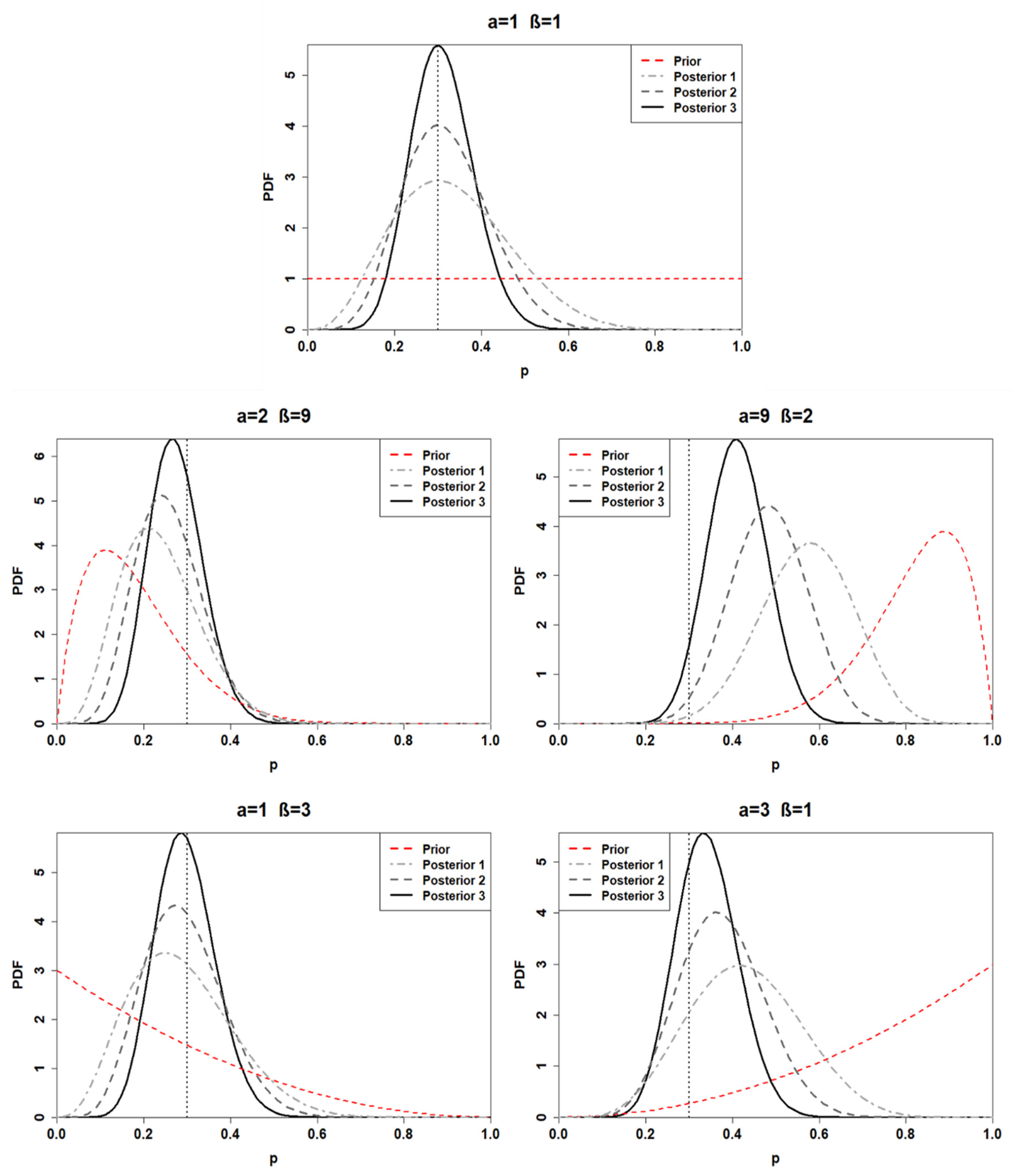
3.1. Prior Choice
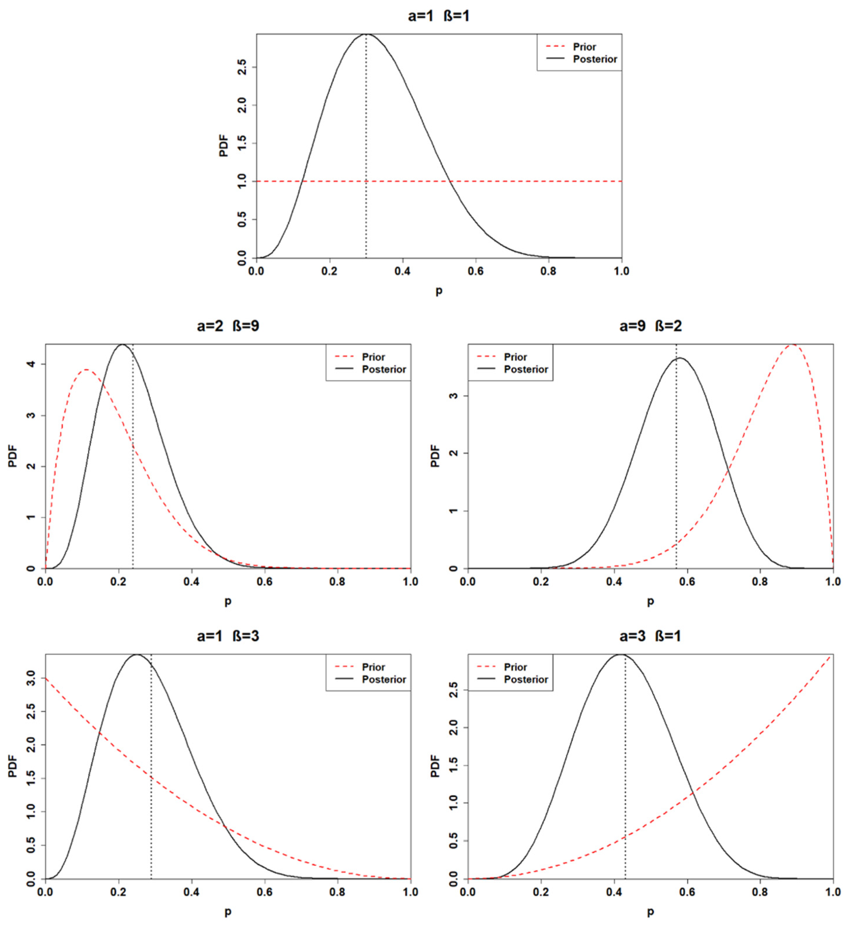
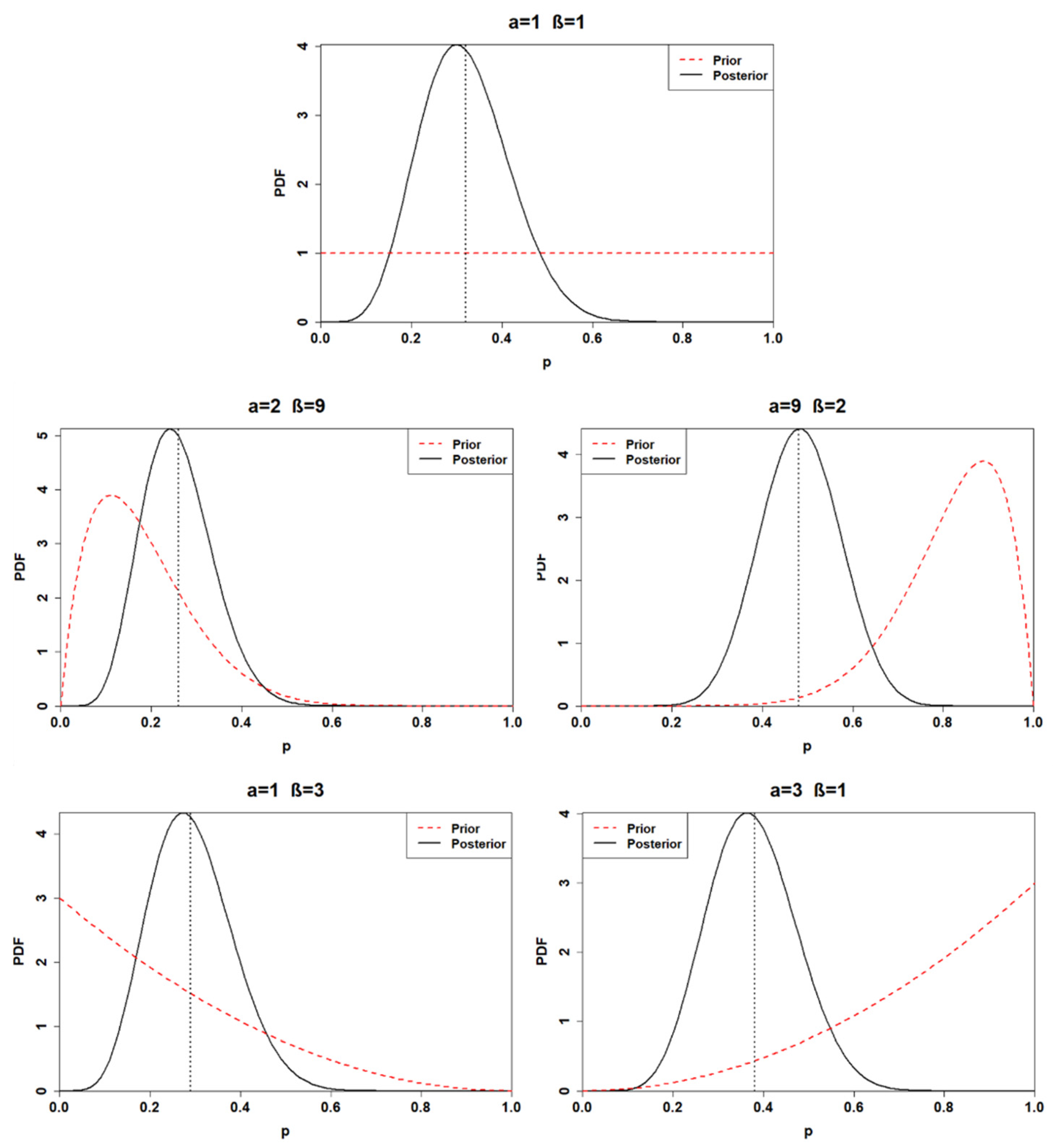
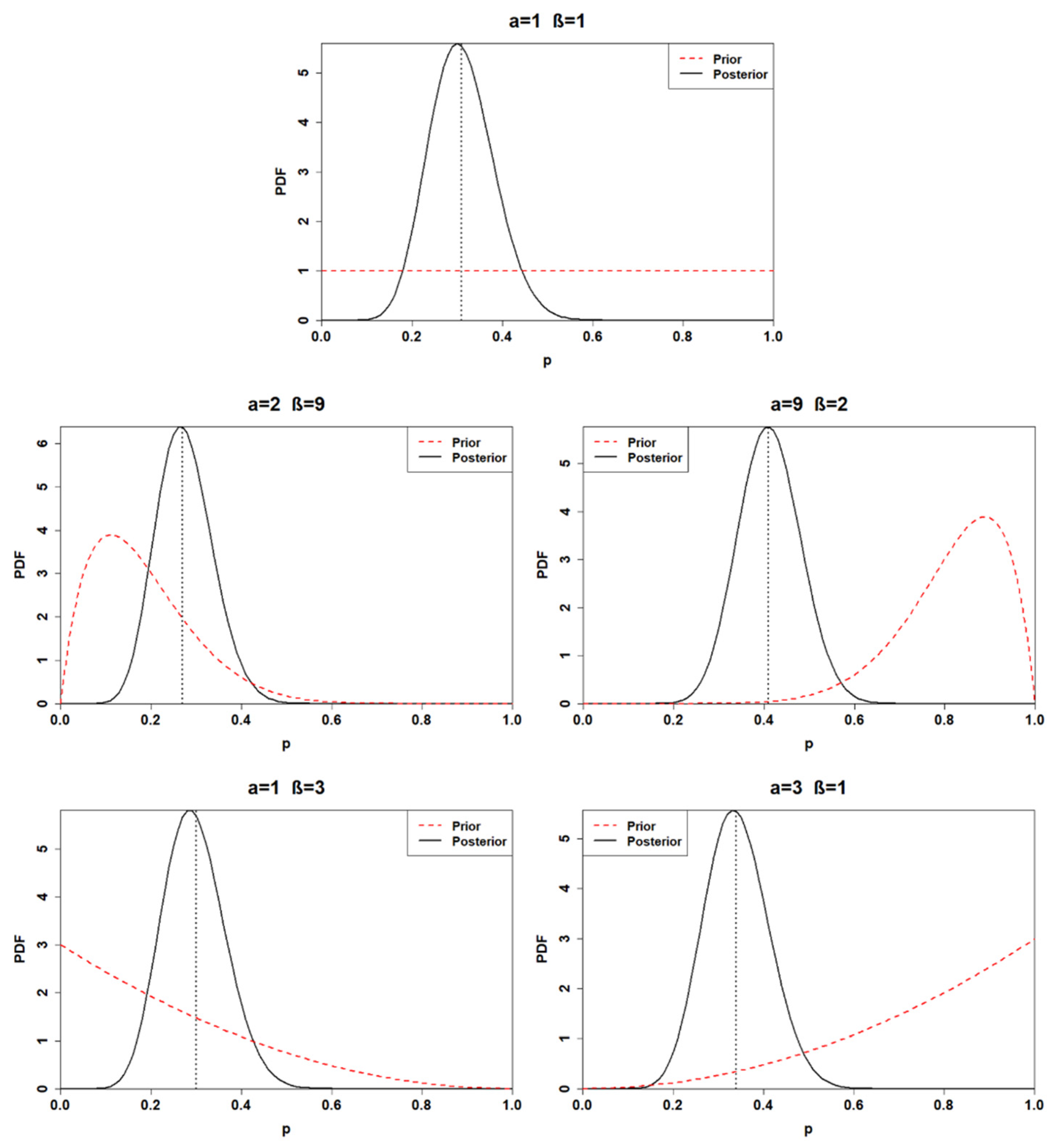
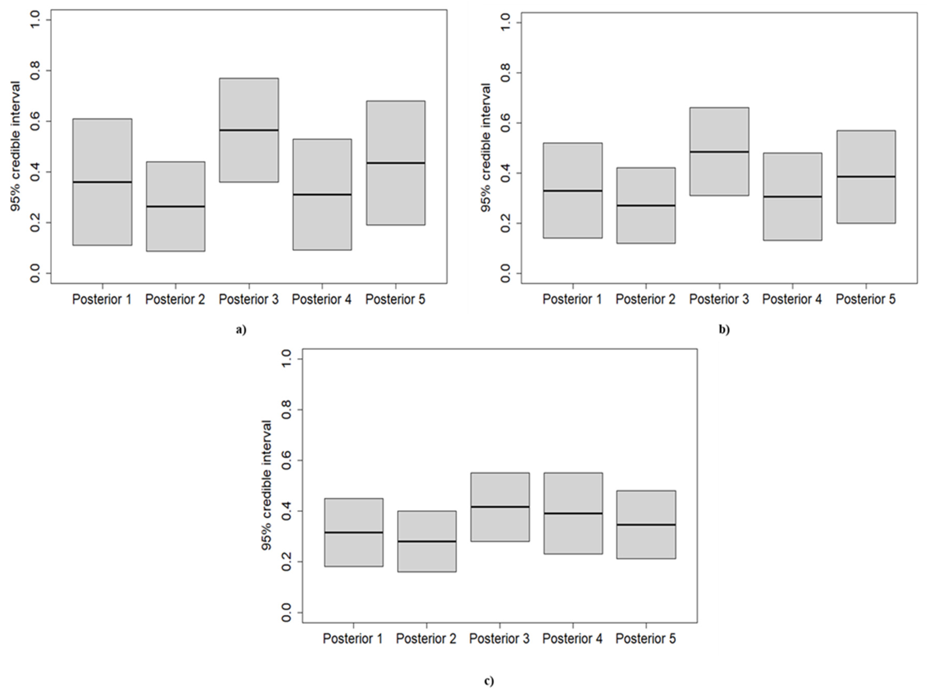
3.2. Posterior Distribution
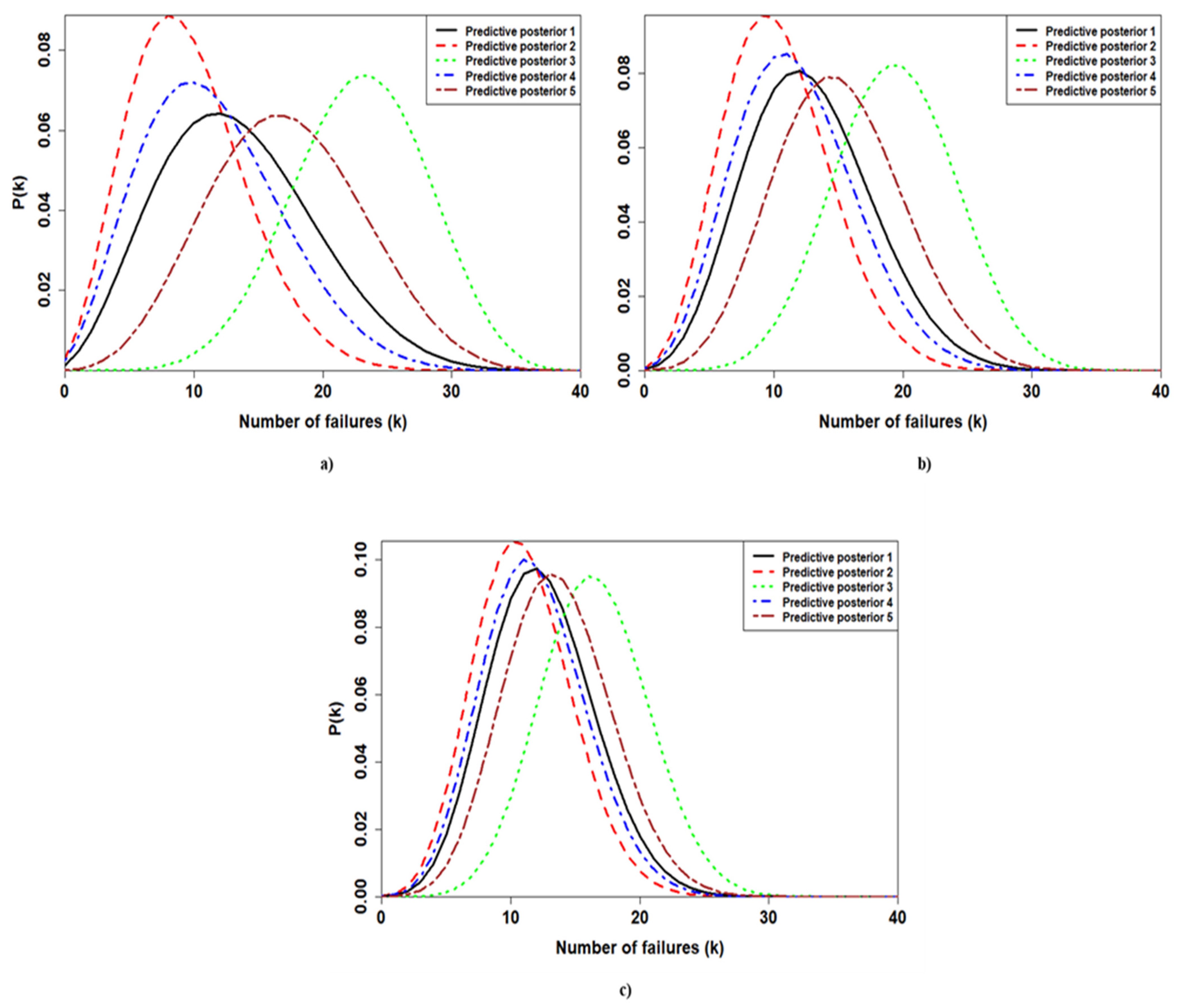
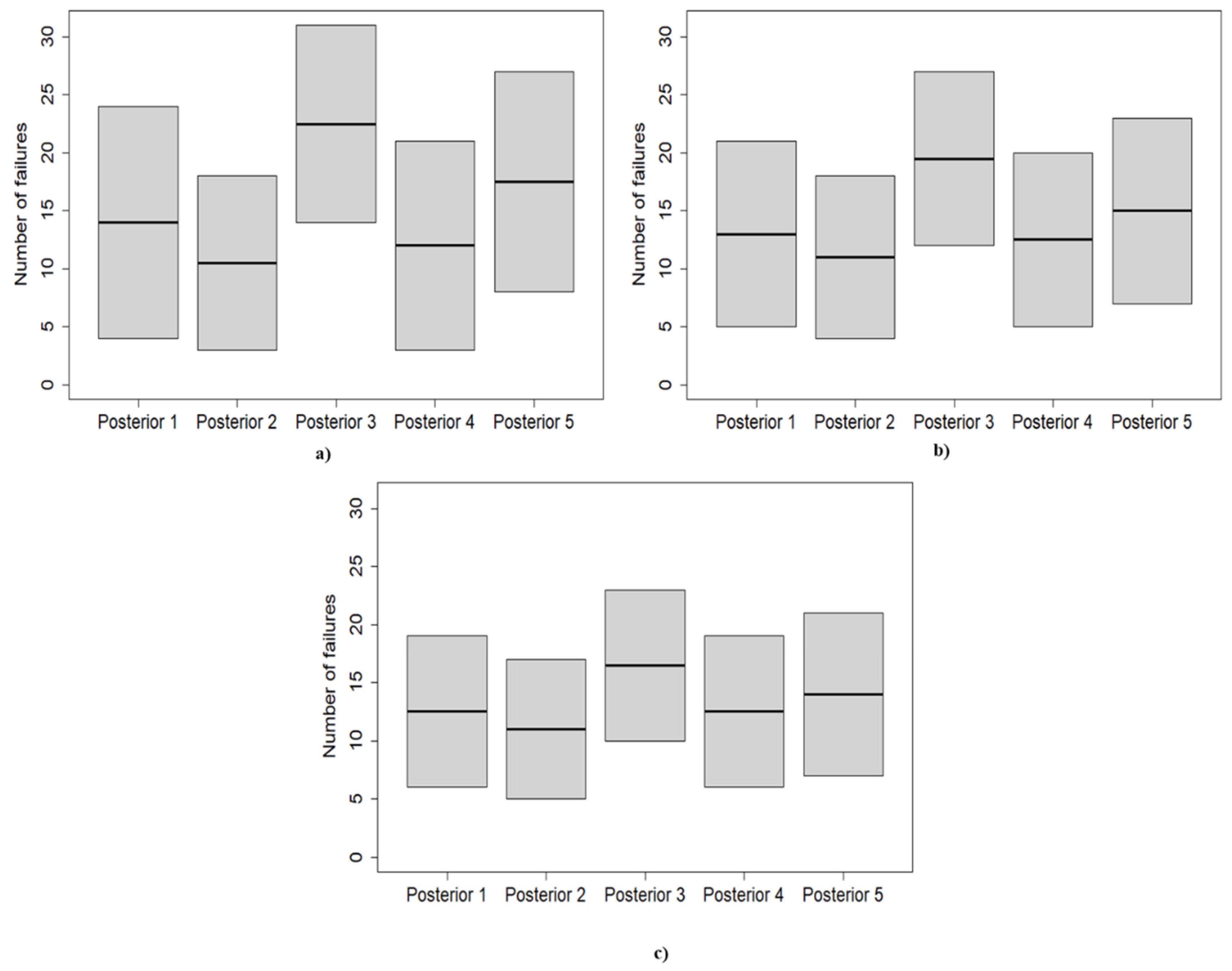
3.3. Predictive Posterior Distribution
4. Discussion
5. Conclusions
Author Contributions
Funding
Institutional Review Board Statement
Informed Consent Statement
Data Availability Statement
Conflicts of Interest
References
- Jaderi, F.; Ibrahim, Z.Z.; Zahiri, M.R. Criticality analysis of petrochemical assets using risk based maintenance and the fuzzy inference system. Process Saf. Environ. Prot. 2019, 121, 312–325. [Google Scholar] [CrossRef]
- Han, Z.Y.; Weng, W.G. Comparison study on qualitative and quantitative risk assessment methods for urban natural gas pipeline network. J. Hazard. Mater. 2011, 189, 509–518. [Google Scholar] [CrossRef]
- Abbasi, T.; Kumar, V.; Tauseef, S.; Abbasi, S. Spread rate of flammable liquids over flat and inclined porous surfaces. J. Chem. Health Saf. 2018, 25, 19–27. [Google Scholar] [CrossRef]
- Abbasi, T.; Abbasi, S.A. The expertise and the practice of loss prevention in the Indian process industry: Some pointers for the third world. Process Saf. Environ. Prot. 2005, 83, 413–420. [Google Scholar] [CrossRef]
- Soltanali, H.; Rohani, A.; Abbaspour-Fard, M.H.; Parida, A.; Farinha, J.T. Development of a risk-based maintenance decision making approach for automotive production line. Int. J. Syst. Assur. Eng. Manag. 2020, 11, 236–251. [Google Scholar] [CrossRef]
- Volkanovski, A.; Čepin, M.; Mavko, B. Application of the fault tree analysis for assessment of power system reliability. Reliab. Eng. Syst. Saf. 2009, 94, 1116–1127. [Google Scholar] [CrossRef]
- Čepin, M.; Mavko, B. A dynamic fault tree. Reliab. Eng. Syst. Saf. 2002, 75, 83–91. [Google Scholar] [CrossRef]
- Purba, J.H.; Lu, J.; Zhang, G.; Pedrycz, W. A fuzzy reliability assessment of basic events of fault trees through qualitative data processing. Fuzzy Sets Syst. 2014, 243, 50–69. [Google Scholar] [CrossRef]
- Mentes, A.; Helvacioglu, I.H. An application of fuzzy fault tree analysis for spread mooring systems. Ocean. Eng. 2011, 38, 285–294. [Google Scholar] [CrossRef]
- Yuhua, D.; Datao, Y. Estimation of failure probability of oil and gas transmission pipelines by fuzzy fault tree analysis. J. Loss Prev. Process. Ind. 2005, 18, 83–88. [Google Scholar] [CrossRef]
- Odell, P.M.; Anderson, K.M.; D’Agostino, R.B. Maximum likelihood estimation for interval-censored data using a Weibull-based accelerated failure time model. Biometrics 1992, 48, 951–959. [Google Scholar] [CrossRef]
- Maier, H.R.; Lence, B.J.; Tolson, B.A.; Foschi, R.O. First-order reliability method for estimating reliability, vulnerability, and resilience. Water Resour. Res. 2001, 37, 779–790. [Google Scholar] [CrossRef]
- Keshtegar, B.; Chakraborty, S. A hybrid self-adaptive conjugate first order reliability method for robust structural reliability analysis. Appl. Math. Model. 2018, 53, 319–332. [Google Scholar] [CrossRef]
- Teixeira, A.; Soares, C.G.; Netto, T.; Estefen, S. Reliability of pipelines with corrosion defects. Int. J. Press. Vessel. Pip. 2008, 85, 228–237. [Google Scholar] [CrossRef]
- Zhang, J.; Du, X. A second-order reliability method with first-order efficiency. J. Mech. Des. 2010, 132, 101006. [Google Scholar] [CrossRef]
- Lee, I.; Noh, Y.; Yoo, D. A novel second-order reliability method (SORM) using noncentral or generalized chi-squared distributions. J. Mech. Des. 2012, 134, 100912. [Google Scholar] [CrossRef]
- Witek, M. Gas transmission pipeline failure probability estimation and defect repairs activities based on in-line inspection data. Eng. Fail. Anal. 2016, 70, 255–272. [Google Scholar] [CrossRef]
- Leoni, L.; BahooToroody, A.; De Carlo, F.; Paltrinieri, N. Developing a risk-based maintenance model for a Natural Gas Regulating and Metering Station using Bayesian Network. J. Loss Prev. Process Ind. 2019, 57, 17–24. [Google Scholar] [CrossRef]
- BahooToroody, A.; Abaei, M.M.; Arzaghi, E.; BahooToroody, F.; De Carlo, F.; Abbassi, R. Multi-level optimization of maintenance plan for natural gas system exposed to deterioration process. J. Hazard. Mater. 2019, 362, 412–423. [Google Scholar] [CrossRef] [PubMed]
- Abbassi, R.; Bhandari, J.; Khan, F.; Garaniya, V.; Chai, S. Developing a quantitative risk-based methodology for maintenance scheduling using Bayesian network. Chem. Eng. Trans. 2016, 48, 235–240. [Google Scholar]
- BahooToroody, A.; Abaiee, M.M.; Gholamnia, R.; Torody, M.B.; Nejad, N.H. Developing a risk-based approach for optimizing human reliability assessment in an offshore operation. Open J. Saf. Sci. Technol. 2016, 6, 25. [Google Scholar] [CrossRef][Green Version]
- Abaei, M.M.; Abbassi, R.; Garaniya, V.; Arzaghi, E.; Toroody, A.B. A dynamic human reliability model for marine and offshore operations in harsh environments. Ocean Eng. 2019, 173, 90–97. [Google Scholar] [CrossRef]
- Golestani, N.; Abbassi, R.; Garaniya, V.; Asadnia, M.; Khan, F. Human reliability assessment for complex physical operations in harsh operating conditions. Process Saf. Environ. Prot. 2020, 140, 1–13. [Google Scholar] [CrossRef]
- Mkrtchyan, L.; Podofillini, L.; Dang, V.N. Bayesian belief networks for human reliability analysis: A review of applications and gaps. Reliab. Eng. Syst. Saf. 2015, 139, 1–16. [Google Scholar] [CrossRef]
- Zhai, S.; Lin, S. Bayesian networks application in multi-state system reliability analysis. In Proceedings of the 2nd International Symposium on Computer, Communication, Control and Automation (ISCCCA-13), Shijiazhuang, China, 22–24 February 2013; Atlantis Press: Paris, France, 2013. [Google Scholar]
- Boudali, H.; Dugan, J.B. A discrete-time Bayesian network reliability modeling and analysis framework. Reliab. Eng. Syst. Saf. 2005, 87, 337–349. [Google Scholar] [CrossRef]
- Torres-Toledano, J.G.; Sucar, L.E. Bayesian networks for reliability analysis of complex systems. In Ibero-American Conference on Artificial Intelligence; Springer: Berlin/Heidelberg, Germany, 1998. [Google Scholar]
- Wu, J.; Zhou, R.; Xu, S.; Wu, Z. Probabilistic analysis of natural gas pipeline network accident based on Bayesian network. J. Loss Prev. Process Ind. 2017, 46, 126–136. [Google Scholar] [CrossRef]
- Abaei, M.M.; Abbassi, R.; Garaniya, V.; Chai, S.; Khan, F. Reliability assessment of marine floating structures using Bayesian network. Appl. Ocean Res. 2018, 76, 51–60. [Google Scholar] [CrossRef]
- Khalaj, S.; BahooToroody, F.; Abaei, M.M.; BahooToroody, A.; De Carlo, F.; Abbassi, R. A methodology for uncertainty analysis of landslides triggered by an earthquake. Comput. Geotech. 2020, 117, 103262. [Google Scholar] [CrossRef]
- Przytula, K.W.; Choi, A. An implementation of prognosis with dynamic bayesian networks. In Proceedings of the 2008 IEEE Aerospace Conference, Big Sky, MT, USA, 1–8 March 2008; IEEE: Piscataway, NJ, USA, 2008. [Google Scholar]
- Chen, C.; Brown, D.; Sconyers, C.; Zhang, B.; Vachtsevanos, G.; Orchard, M.E. An integrated architecture for fault diagnosis and failure prognosis of complex engineering systems. Expert Syst. Appl. 2012, 39, 9031–9040. [Google Scholar] [CrossRef]
- Patrick, R.; Orchard, M.E.; Zhang, B.; Koelemay, M.D.; Kacprzynski, G.J.; Ferri, A.A.; Vachtsevanos, G.J. An integrated approach to helicopter planetary gear fault diagnosis and failure prognosis. In Proceedings of the 2007 IEEE Autotestcon, Baltimore, MD, USA, 17–20 September 2007; IEEE: Piscataway, NJ, USA, 2007. [Google Scholar]
- Zarate, B.A.; Caicedo, J.M.; Yu, J.; Ziehl, P. Bayesian model updating and prognosis of fatigue crack growth. Eng. Struct. 2012, 45, 53–61. [Google Scholar] [CrossRef]
- Sun, F.; Li, X.; Liao, H.; Zhang, X. A Bayesian least-squares support vector machine method for predicting the remaining useful life of a microwave component. Adv. Mech. Eng. 2017, 9, 1687814016685963. [Google Scholar] [CrossRef]
- Bhandari, J.; Abbassi, R.; Garaniya, V.; Khan, F. Risk analysis of deepwater drilling operations using Bayesian network. J. Loss Prev. Process Ind. 2015, 38, 11–23. [Google Scholar] [CrossRef]
- Liu, Z.; Liu, Y. A Bayesian network based method for reliability analysis of subsea blowout preventer control system. J. Loss Prev. Process Ind. 2019, 59, 44–53. [Google Scholar] [CrossRef]
- BahooToroody, A.; Abaei, M.M.; Arzaghi, E.; Song, G.; De Carlo, F.; Paltrinieri, N.; Abbassi, R. On reliability challenges of repairable systems using hierarchical bayesian inference and maximum likelihood estimation. Process Saf. Environ. Prot. 2020, 135, 157–165. [Google Scholar] [CrossRef]
- Musleh, R.M.; Helu, A. Estimation of the inverse Weibull distribution based on progressively censored data: Comparative study. Reliab. Eng. Syst. Saf. 2014, 131, 216–227. [Google Scholar] [CrossRef]
- Khakzad, N.; Khan, F.; Amyotte, P. Safety analysis in process facilities: Comparison of fault tree and Bayesian network approaches. Reliab. Eng. Syst. Saf. 2011, 96, 925–932. [Google Scholar] [CrossRef]
- Li, H.; Soares, C.G.; Huang, H.-Z. Reliability analysis of a floating offshore wind turbine using Bayesian Networks. Ocean Eng. 2020, 217, 107827. [Google Scholar] [CrossRef]
- Spiegelhalter, D.; Thomas, A.; Best, N.; Lunn, D. OpenBUGS User Manual, Version 3.0.2; MRC Biostatistics Unit: Cambridge, UK, 2007. [Google Scholar]
- Robert, C. The Bayesian Choice: From Decision-Theoretic Foundations to Computational Implementation; Springer Science & Business Media: Berlin/Heidelberg, Germany, 2007. [Google Scholar]
- Kumari, P.; Lee, D.; Wang, Q.; Karim, M.N.; Kwon, J.S.-I. Root cause analysis of key process variable deviation for rare events in the chemical process industry. Ind. Eng. Chem. Res. 2020, 59, 10987–10999. [Google Scholar] [CrossRef]
- Leoni, L.; De Carlo, F.; Sgarbossa, F.; Paltrinieri, N. Comparison of Risk-based Maintenance Approaches Applied to a Natural Gas Regulating and Metering Station. Chem. Eng. Trans. 2020, 82, 115–120. [Google Scholar]
- Leoni, L.; BahooToroody, A.; Abaei, M.M.; De Carlo, F.; Paltrinieri, N.; Sgarbossa, F. On hierarchical bayesian based predictive maintenance of autonomous natural gas regulating operations. Process Saf. Environ. Prot. 2021, 147, 115–124. [Google Scholar] [CrossRef]
- BahooToroody, F.; Khalaj, S.; Leoni, L.; De Carlo, F.; Di Bona, G.; Forcina, A. Reliability Estimation of Reinforced Slopes to Prioritize Maintenance Actions. Int. J. Environ. Res. Public Health 2021, 18, 373. [Google Scholar] [CrossRef]
- BahooToroody, A.; De Carlo, F.; Paltrinieri, N.; Tucci, M.; Van Gelder, P. Bayesian Regression Based Condition Monitoring Approach for Effective Reliability Prediction of Random Processes in Autonomous Energy Supply Operation. Reliab. Eng. Syst. Saf. 2020, 201, 106966. [Google Scholar] [CrossRef]
- BahooToroody, A.; Abaei, M.M.; BahooToroody, F.; De Carlo, F.; Abbassi, R.; Khalaj, S. A condition monitoring based signal filtering approach for dynamic time dependent safety assessment of natural gas distribution process. Process Saf. Environ. Prot. 2019, 123, 335–343. [Google Scholar] [CrossRef]
- Yang, M.; Khan, F.I.; Lye, L. Precursor-based hierarchical Bayesian approach for rare event frequency estimation: A case of oil spill accidents. Process Saf. Environ. Prot. 2013, 91, 333–342. [Google Scholar] [CrossRef]
- Abaei, M.M.; Arzaghi, E.; Abbassi, R.; Garaniya, V.; Javanmardi, M.; Chai, S. Dynamic reliability assessment of ship grounding using Bayesian Inference. Ocean Eng. 2018, 159, 47–55. [Google Scholar] [CrossRef]
- Andrade, A.R.; Teixeira, P.F. Statistical modelling of railway track geometry degradation using hierarchical Bayesian models. Reliab. Eng. Syst. Saf. 2015, 142, 169–183. [Google Scholar] [CrossRef]
- Yu, R.; Abdel-Aty, M. Investigating different approaches to develop informative priors in hierarchical Bayesian safety performance functions. Accid. Anal. Prev. 2013, 56, 51–58. [Google Scholar] [CrossRef]
- Kelly, D.L.; Smith, C.L. Bayesian inference in probabilistic risk assessment—the current state of the art. Reliab. Eng. Syst. Saf. 2009, 94, 628–643. [Google Scholar] [CrossRef]
- El-Gheriani, M.; Khan, F.; Chen, D.; Abbassi, R. Major accident modelling using spare data. Process Saf. Environ. Prot. 2017, 106, 52–59. [Google Scholar] [CrossRef]
- Kelly, D.; Smith, C. Bayesian Inference for Probabilistic Risk Assessment: A Practitioner’s Guidebook; Springer Science & Business Media: Berlin/Heidelberg, Germany, 2011. [Google Scholar]
- Gelman, A.; Carlin, J.B.; Stern, H.S.; Dunson, D.B.; Vehtari, A.; Rubin, D.B. Bayesian Data Analysis; CRC Press: Boca Raton, FL, USA, 2013. [Google Scholar]
- Yahya, W.; Olaniran, O.; Ige, S. On Bayesian conjugate normal linear regression and ordinary least square regression methods: A Monte Carlo study. Ilorin J. Sci. 2014, 1, 216–227. [Google Scholar]


| Sample | # Observations (n) | # Failures (k) |
|---|---|---|
| Sample 1 | 10 | 3 |
| Sample 2 | 20 | 6 |
| Sample 3 | 40 | 12 |
| Beta Prior Distribution (BPD) | Hyper-Parameters | Prior Mean | Prior Variance | |
|---|---|---|---|---|
| Alpha | Beta | |||
| BPD 1 (non-informative) | 1 | 1 | 0.5 | 0.08 |
| BPD 2 (very reliable) | 2 | 9 | 0.18 | 0.01 |
| BPD 3 (very unreliable) | 9 | 2 | 0.82 | 0.01 |
| BPD 4 (quite reliable) | 1 | 3 | 0.25 | 0.04 |
| BPD 5 (quite unreliable) | 3 | 1 | 0.75 | 0.04 |
| # Posterior | Alpha | Beta | Posterior Mean | 95% Posterior Interval for p |
|---|---|---|---|---|
| Posterior1 | 4 | 8 | 0.33 | [0.11, 0.61] |
| Posterior2 | 5 | 16 | 0.24 | [0.086, 0.44] |
| Posterior3 | 12 | 9 | 0.57 | [0.36, 0.77] |
| Posterior4 | 4 | 10 | 0.29 | [0.09, 0.53] |
| Posterior5 | 6 | 8 | 0.43 | [0.19, 0.68] |
| # Posterior | Alpha | Beta | Posterior Mean | 95% Posterior Interval for p |
|---|---|---|---|---|
| Posterior1 | 7 | 15 | 0.32 | [0.14, 0.52] |
| Posterior2 | 8 | 23 | 0.26 | [0.12, 0.42] |
| Posterior3 | 15 | 16 | 0.48 | [0.31, 0.66] |
| Posterior4 | 7 | 17 | 0.29 | [0.13, 0.48] |
| Posterior5 | 9 | 15 | 0.38 | [0.20, 0.57] |
| # Posterior | Alpha | Beta | Posterior Mean | 95% Posterior Interval for p |
|---|---|---|---|---|
| Posterior1 | 13 | 29 | 0.31 | [0.18, 0.45] |
| Posterior2 | 14 | 37 | 0.27 | [0.16, 0.40] |
| Posterior3 | 21 | 30 | 0.41 | [0.28, 0.55] |
| Posterior4 | 13 | 31 | 0.30 | [0.23, 0.55] |
| Posterior5 | 15 | 29 | 0.34 | [0.21, 0.48] |
| First Application | Second Application | Third Application | ||||
|---|---|---|---|---|---|---|
| # Posterior | 0.05 | 0.95 | 0.05 | 0.95 | 0.05 | 0.95 |
| Posterior 1 | 4 | 24 | 5 | 21 | 6 | 19 |
| Posterior 2 | 3 | 18 | 4 | 18 | 5 | 17 |
| Posterior 3 | 14 | 31 | 12 | 27 | 10 | 23 |
| Posterior 4 | 3 | 21 | 5 | 20 | 6 | 19 |
| Posterior 5 | 8 | 27 | 7 | 23 | 7 | 21 |
Publisher’s Note: MDPI stays neutral with regard to jurisdictional claims in published maps and institutional affiliations. |
© 2021 by the authors. Licensee MDPI, Basel, Switzerland. This article is an open access article distributed under the terms and conditions of the Creative Commons Attribution (CC BY) license (http://creativecommons.org/licenses/by/4.0/).
Share and Cite
Leoni, L.; BahooToroody, F.; Khalaj, S.; Carlo, F.D.; BahooToroody, A.; Abaei, M.M. Bayesian Estimation for Reliability Engineering: Addressing the Influence of Prior Choice. Int. J. Environ. Res. Public Health 2021, 18, 3349. https://doi.org/10.3390/ijerph18073349
Leoni L, BahooToroody F, Khalaj S, Carlo FD, BahooToroody A, Abaei MM. Bayesian Estimation for Reliability Engineering: Addressing the Influence of Prior Choice. International Journal of Environmental Research and Public Health. 2021; 18(7):3349. https://doi.org/10.3390/ijerph18073349
Chicago/Turabian StyleLeoni, Leonardo, Farshad BahooToroody, Saeed Khalaj, Filippo De Carlo, Ahmad BahooToroody, and Mohammad Mahdi Abaei. 2021. "Bayesian Estimation for Reliability Engineering: Addressing the Influence of Prior Choice" International Journal of Environmental Research and Public Health 18, no. 7: 3349. https://doi.org/10.3390/ijerph18073349
APA StyleLeoni, L., BahooToroody, F., Khalaj, S., Carlo, F. D., BahooToroody, A., & Abaei, M. M. (2021). Bayesian Estimation for Reliability Engineering: Addressing the Influence of Prior Choice. International Journal of Environmental Research and Public Health, 18(7), 3349. https://doi.org/10.3390/ijerph18073349