
Multi-Scenario Analysis of Habitat Quality in the Yellow River Delta by Coupling FLUS with InVEST Model


Abstract
1. Introduction
2. Material and Methods
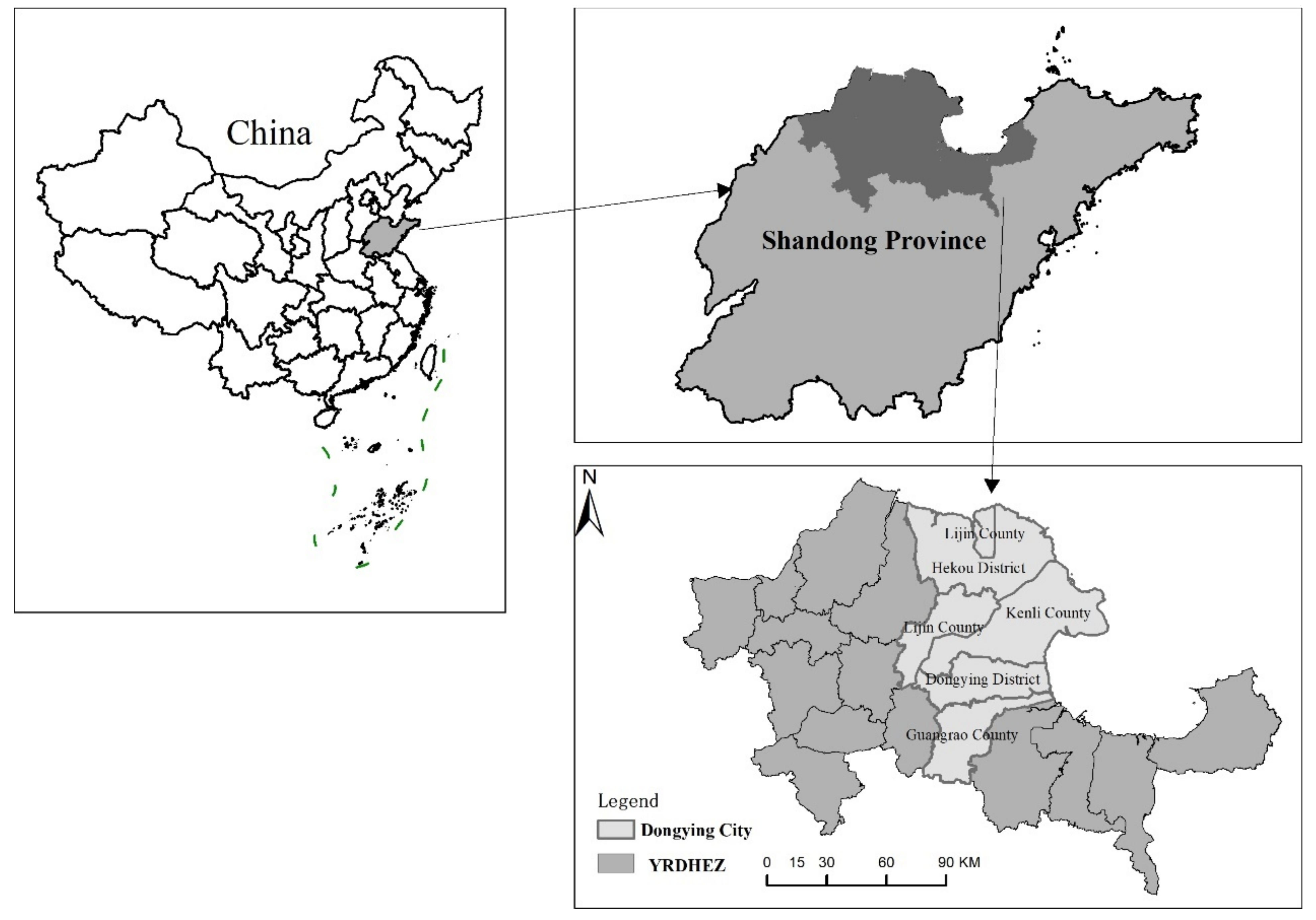
2.1. Study Area
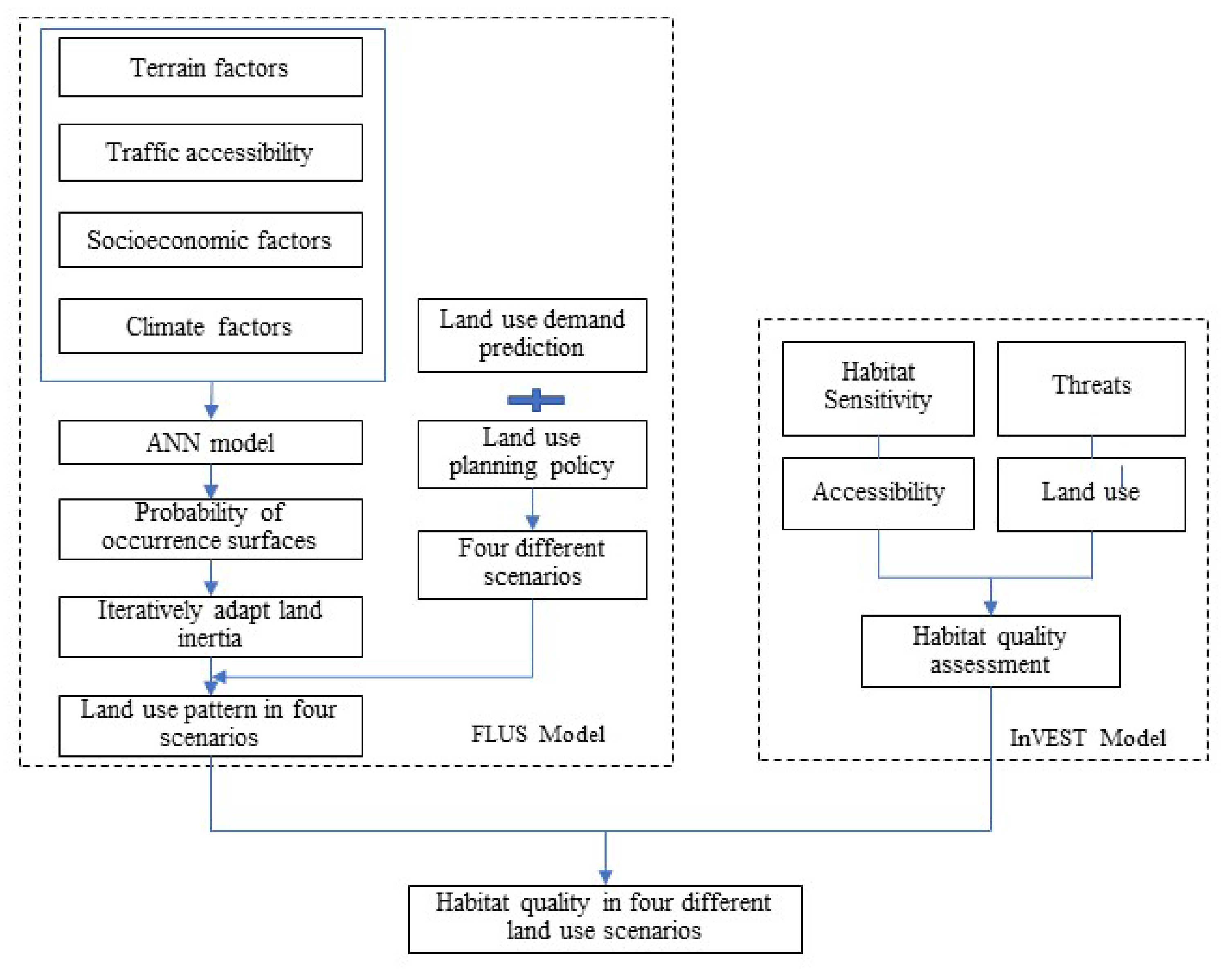
2.2. Methodology
2.2.1. Defining Scenarios and Calculating Future Land Use Demand
2.2.2. Simulating Future Land Use Using FLUS Model
Calculation of Probability-of-Occurrence Estimation Using Artificial Neural Networks
Self-Adaptive Inertia and Competition Mechanism
2.2.3. Assessing Habitat Quality Using InVEST Model
3. Results Analysis
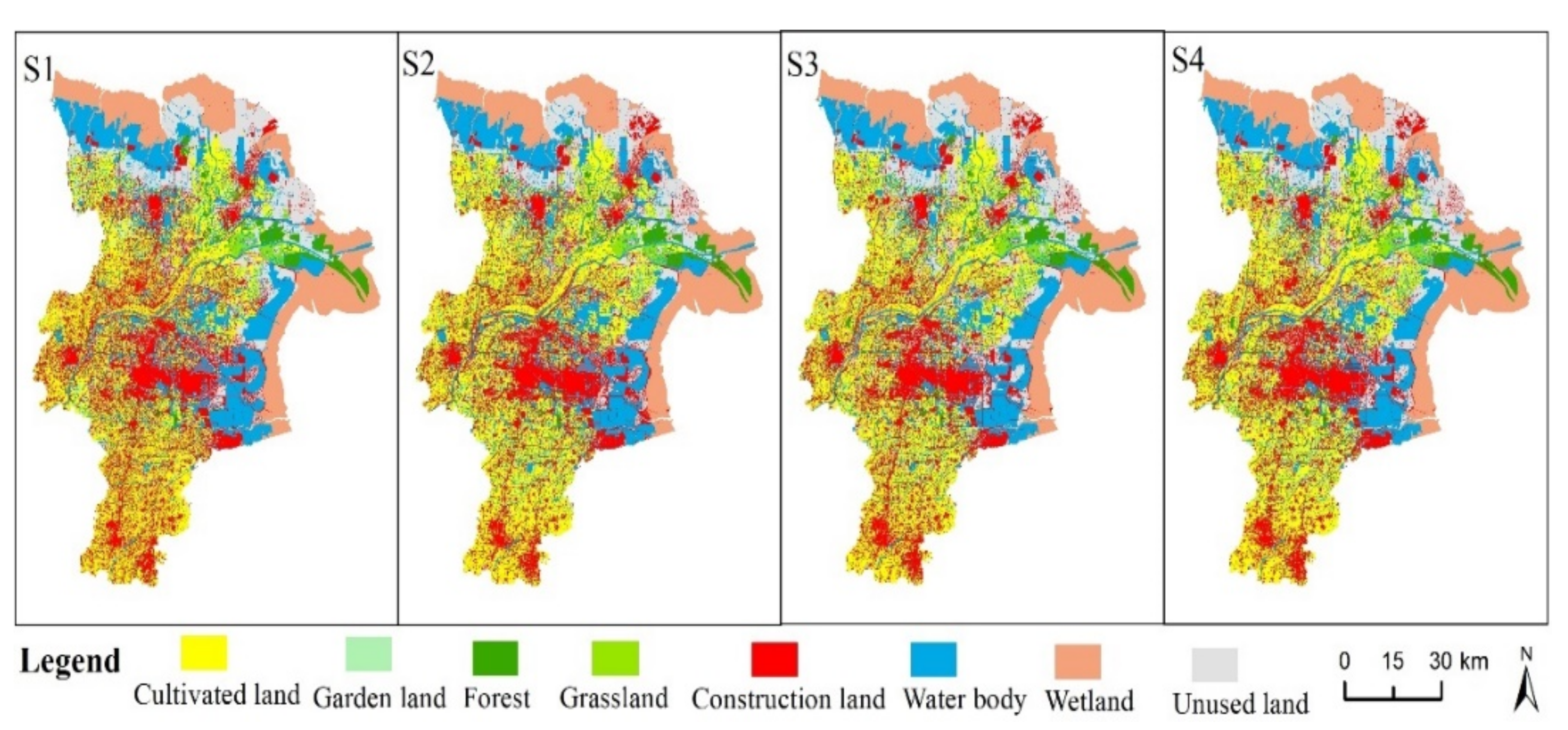
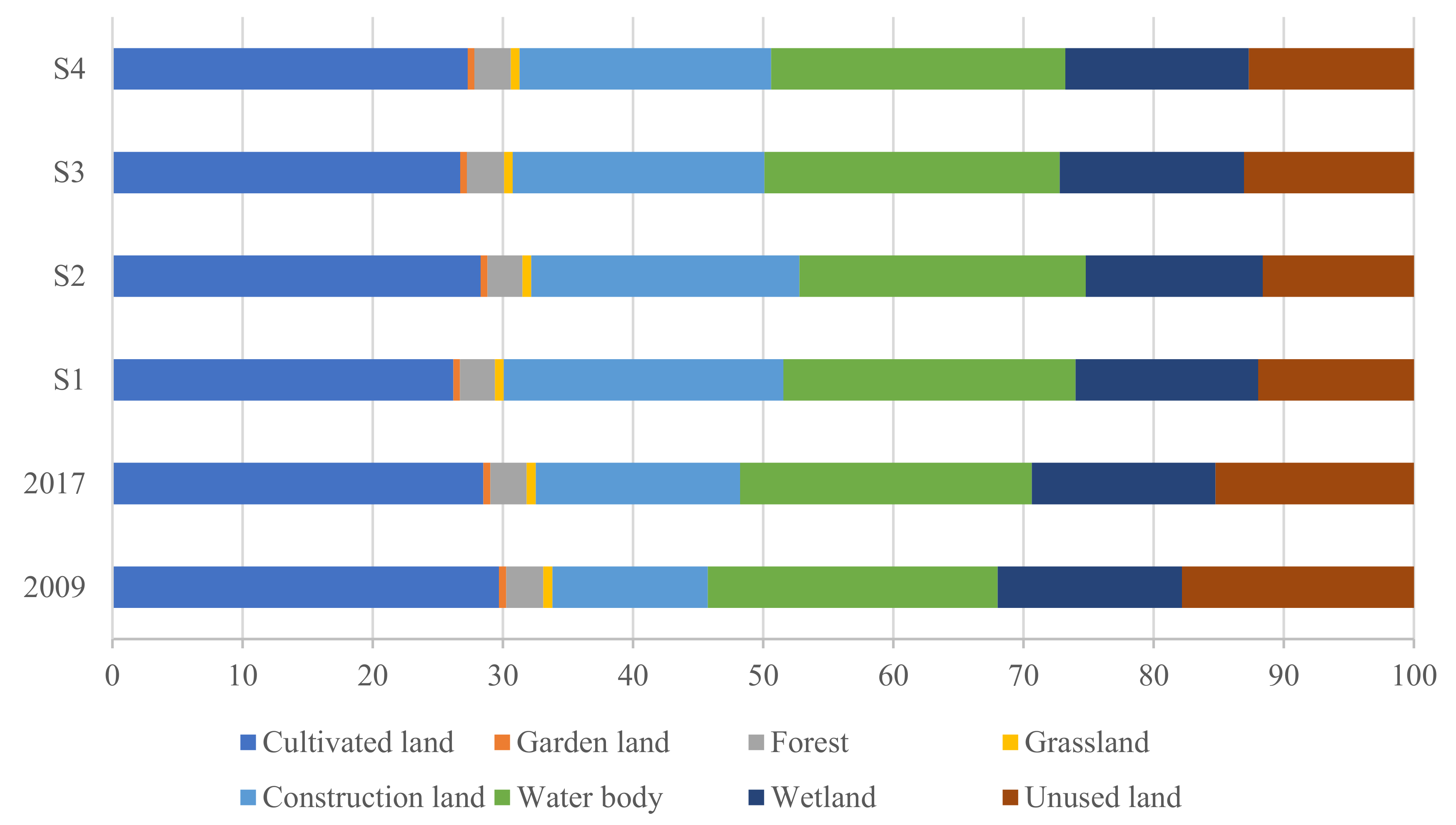
3.1. Multi-Scenario Simulation for Future Land Use
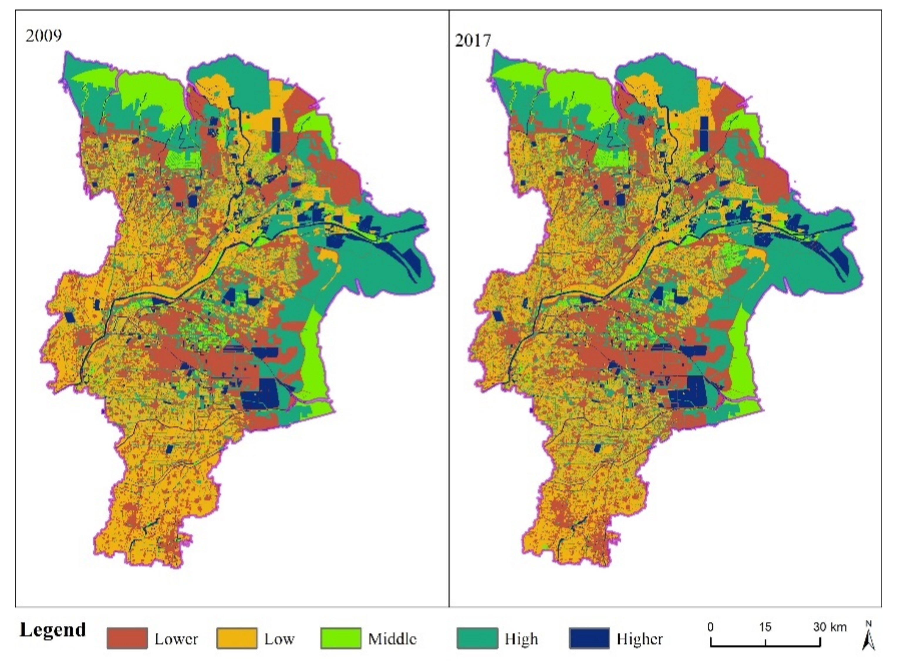
3.2. Habitat Quality Assessment under Different Scenarios
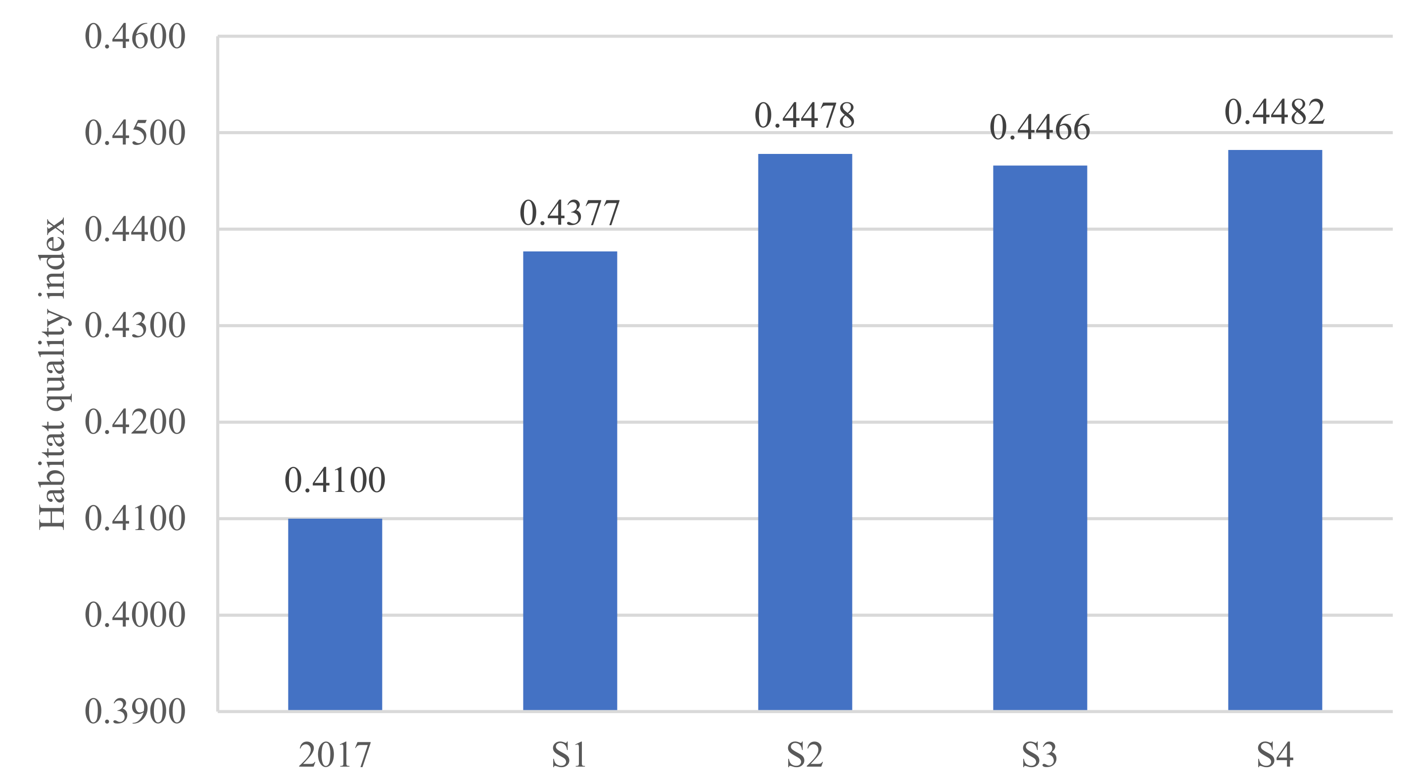
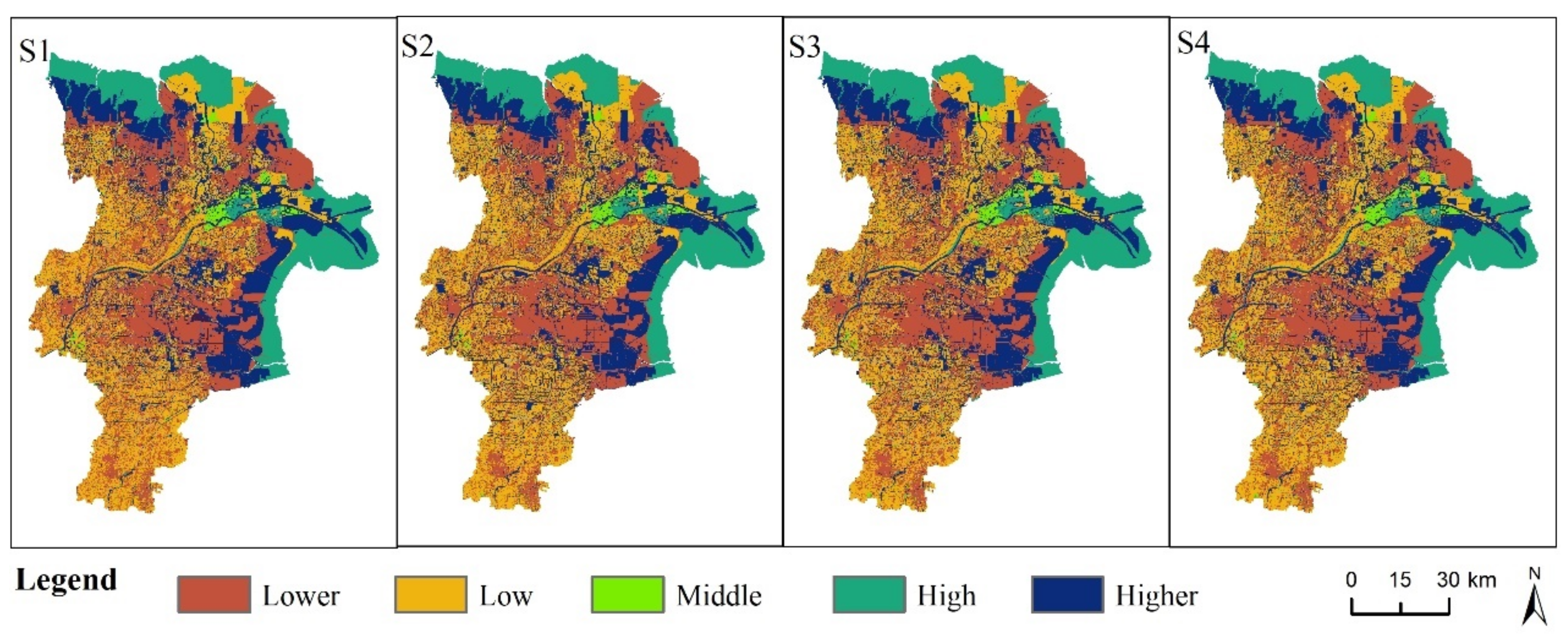
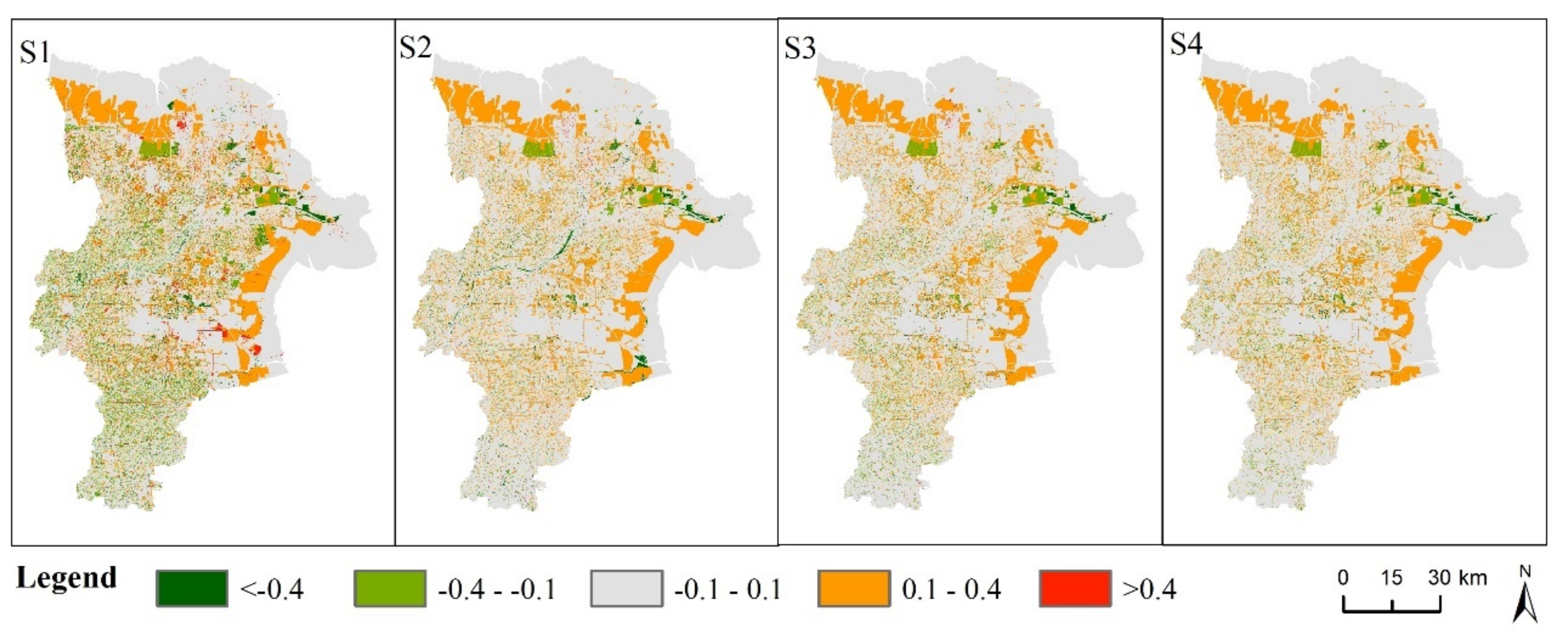
3.3. Comparison of Habitat Quality under Four Scenarios
4. Discussion
4.1. Future Land Use and Habitat Quality
4.2. Impacts of Future Land Use on Habitat Quality
4.3. Policy Implications
4.4. Limitations and Improvement
5. Conclusions
Author Contributions
Funding
Institutional Review Board Statement
Informed Consent Statement
Data Availability Statement
Conflicts of Interest
References
- Butchart, S.H.; Walpole, M.; Collen, B.; Van Strien, A.; Scharlemann, J.P.; Almond, R.E.; Baillie, J.E.; Bomhard, B.; Brown, C.; Bruno, J.; et al. Global biodiversity: Indicators of recent declines. Science 2010, 328, 1164–1168. [Google Scholar] [CrossRef] [PubMed]
- Terrado, M.; Sabater, S.; Chaplin-Kramer, B.; Mandle, L.; Ziv, G.; Acuna, V. Model development for the assessment of terrestrial and aquatic habitat quality in conservation planning. Sci. Total Environ. 2016, 540, 63–70. [Google Scholar] [CrossRef] [PubMed]
- Nelson, E.; Mendoza, G.; Regetz, J.; Polasky, S.; Tallis, H.; Cameron, D.R.; Chan, K.M.A.; Daily, G.C.; Goldstein, J.; Kareiva, P.M.; et al. Modeling multiple ecosystem services, biodiversity conservation, commodity production, and tradeoffs at landscape scales. Front. Ecol. Environ. 2009, 7, 4–11. [Google Scholar] [CrossRef]
- Goldstein, J.H.; Caldarone, G.; Duarte, T.K.; Ennaanay, D.; Hannahs, N.; Mendoza, G.; Polasky, S.; Wolny, S.; Daily, G.C. Integrating ecosystem-service tradeoffs into land-use decisions. Proc. Natl. Acad. Sci. USA 2012, 109, 7565–7570. [Google Scholar] [CrossRef] [PubMed]
- Sala, O.E.; Chapin, F.S.; Armesto, J.J.; Berlow, E.L.; Bloomfield, J.; Dirzo, R.; Hubersanwald, E.; Huenneke, L.F.; Jackson, R.B.; Kinzig, A.P.J.S. Global biodiversity scenarios for the year 2100. Science 2000, 287, 1770–1774. [Google Scholar] [CrossRef] [PubMed]
- MEPC. China National Biodiversity Conservation Strategy and Action Plans 2011–2030; Chinese Environmental Science Press: Beijing, China, 2011. [Google Scholar]
- Liu, C.H.; Lun, Y. Progress, achievements and prospects of biodiversity protection in Yunnan Province. Biodivers. Sci. 2020. [Google Scholar] [CrossRef]
- Lawler, J.J.; Lewis, D.J.; Nelson, E.; Plantinga, A.J.; Polasky, S.; Withey, J.C.; Helmers, D.P.; Martinuzzi, S.; Pennington, D.; Radeloff, V.C. Projected land-use change impacts on ecosystem services in the United States. Proc. Natl. Acad. Sci. USA 2014, 111, 7492–7497. [Google Scholar] [CrossRef]
- Sun, X.; Crittenden, J.C.; Li, F.; Lu, Z.; Dou, X. Urban expansion simulation and the spatio-temporal changes of ecosystem services, a case study in Atlanta Metropolitan area, USA. Sci. Total Environ. 2018, 622, 974–987. [Google Scholar] [CrossRef]
- Huang, Q.; Zhao, X.; He, C.; Yin, D.; Meng, S. Impacts of urban expansion on wetland ecosystem services in the context of hosting the Winter Olympics: A scenario simulation in the Guanting Reservoir Basin, China. Reg. Environ. Chang. 2019, 19, 2365–2379. [Google Scholar] [CrossRef]
- Seto, K.C.; Fragkias, M.; Güneralp, B.; Reilly, M.K. A Meta-Analysis of Global Urban Land Expansion. PLoS ONE 2011, 6, e23777. [Google Scholar] [CrossRef]
- Seto, K.C.; Giineralp, B.; Hutyra, L.R. Global forecasts of urban expansion to 2030 and direct impacts on biodiversity and carbon pools. Proc. Natl. Acad. Sci. USA 2012, 109, 16083–16088. [Google Scholar] [CrossRef] [PubMed]
- Wu, J.; Cao, Q.; Shi, S.; Huang, X.; Lu, Z. Spatio-temporal variability of habitat quality in Beijing-Tianjin-Hebei Area based on land use change. Chin. J. Appl. Ecol. 2015, 26, 3457–3466. [Google Scholar]
- Huang, M.Y.; Yue, W.Z.; Feng, S.R.; Zhang, J.H. Spatial-temporal evolution of habitat quality and analysis of landscape patterns in Dabie Mountain area of west Anhui province based on InVEST model. Acta Ecol. Sin. 2020, 40, 2895–2906. [Google Scholar]
- Wang, L.Z.; Lyons, J.; Kanehl, P.; Gatti, R. Influences of watershed land use on habitat quality and biotic integrity in Wisconsin streams. Fisheries 1997, 22, 6–12. [Google Scholar] [CrossRef]
- Zhong, L.N.; Wang, J. Evaluation on effect of land consolidation on habitat quality based on InVEST model. Trans. CSAE 2017, 33, 250–255. [Google Scholar]
- Bai, L.; Xiu, C.; Feng, X.; Liu, D. Influence of urbanization on regional habitat quality: A case study of Changchun City. Habitat Int. 2019, 93, 102042. [Google Scholar] [CrossRef]
- Zhang, Y.; Chen, R.; Wang, Y. Tendency of land reclamation in coastal areas of Shanghai from 1998 to 2015. Land Use Policy 2020, 91, 104370. [Google Scholar] [CrossRef]
- Liu, Y.; Zhou, Y.; Du, Y. Study on the Spatio-Temporal Patterns of Habitat Quality and Its Terrain Gradient Effects of the Middle of the Yangtze River Economic Belt Based on InVEST Model. Resour. Environ. Yangtze Basin 2019, 28, 2429–2440. [Google Scholar]
- Polasky, S.; Nelson, E.; Pennington, D.; Johnson, K.A. The Impact of Land-Use Change on Ecosystem Services, Biodiversity and Returns to Landowners: A Case Study in the State of Minnesota. Environ. Resour. Econ. 2011, 48, 219–242. [Google Scholar] [CrossRef]
- Guillem, E.E.; Murray-Rust, D.; Robinson, D.T.; Barnes, A.; Rounsevell, M.D.A. Modelling farmer decision-making to anticipate tradeoffs between provisioning ecosystem services and biodiversity. Agric. Syst. 2015, 137, 12–23. [Google Scholar] [CrossRef]
- Asadolahi, Z.; Salmanmahiny, A.; Sakieh, Y.; Mirkarimi, S.H.; Baral, H.; Azimi, M. Dynamic trade-off analysis of multiple ecosystem services under land use change scenarios: Towards putting ecosystem services into planning in Iran. Ecol. Complex. 2018, 36, 250–260. [Google Scholar] [CrossRef]
- Gueneralp, B.; Seto, K.C. Futures of global urban expansion: Uncertainties and implications for biodiversity conservation. Environ. Res. Lett. 2013, 8, 014025. [Google Scholar] [CrossRef]
- Aneseyee, A.B.; Noszczyk, T.; Soromessa, T.; Elias, E. The InVEST Habitat Quality Model Associated with Land Use/Cover Changes: A Qualitative Case Study of the Winike Watershed in the Omo-Gibe Basin, Southwest Ethiopia. Remote Sens. 2020, 12, 1103. [Google Scholar] [CrossRef]
- Lei, J.C.; Liu, J.X.; Yong, F.; Liu, H.M.; Wu, J.; Ding, H.; Wang, J.M.; Wu, S.Q.; Cheng, S.; Cui, P. Multi- Scenario Ecosystem Service Assessment of Wuma River Valley Based on CLUE- S and InVEST Models. J. Ecol. Rural Environ. 2017, 33, 1084–1093. [Google Scholar]
- Wang, C.D.; Wang, Y.T.; Wang, R.Q.; Zheng, P.M. Modeling and evaluating land-use/land-cover change for urban planning and sustainability: A case study of Dongying city, China. J. Clean. Prod. 2018, 172, 1529–1534. [Google Scholar] [CrossRef]
- Wang, C.D.; Wang, Y.T.; Geng, Y.; Wang, R.Q.; Zhang, J.Y. Measuring regional sustainability with an integrated social-economic-natural approach: A case study of the Yellow River Delta region of China. J. Clean. Prod. 2016, 114, 189–198. [Google Scholar] [CrossRef]
- Dongying Government. Dongying Statistical Yearbook 2018; Yellow River Press: Jinan, China, 2018.
- Li, X.W.; Hou, X.Y.; Song, Y.; Shan, K.; Zhu, S.Y.; Yu, X.B.; Mo, X.Q. Assessing Changes of Habitat Quality for Shorebirds in Stopover Sites: A Case Study in Yellow River Delta, China. Wetlands 2018, 39, 67–77. [Google Scholar] [CrossRef]
- Yuan, X.; Sun, Y.; Wang, J.; Yu, L. Comprehensive utilization of water resources in the Yellow River Delta for waterfowl habitat restoration. Resour. Sci. 2020, 42, 104–114. [Google Scholar] [CrossRef]
- Liu, X.P.; Liang, X.; Li, X.; Xu, X.C.; Ou, J.P.; Chen, Y.M.; Li, S.Y.; Wang, S.J.; Pei, F.S. A future land use simulation model (FLUS) for simulating multiple land use scenarios by coupling human and natural effects. Landsc. Urban Plan. 2017, 168, 94–116. [Google Scholar] [CrossRef]
- Liang, X.; Liu, X.P.; Li, X.; Chen, Y.M.; Tian, H.; Yao, Y. Delineating multi-scenario urban growth boundaries with a CA-based FLUS model and morphological method. Landsc. Urban Plan. 2018, 177, 47–63. [Google Scholar] [CrossRef]
- Peng, Y.F. Optimization Simulation of City Land Use in the Context of Ecological Security—A Case Study of Shenzhen City; Wuhan University: Wuhan, China, 2018. [Google Scholar]
- Liu, X.J.; Li, X.; Liang, X.; Shi, H.; Ou, J.P. Simulating the Change of Terrestrial Carbon Storage in China Based on the FLUS-InVEST Model. Trop. Geogr. 2019, 39, 397–409. [Google Scholar]
- Li, J.Y.; Gong, J.; Guldmann, J.M.; Li, S.C.; Zhu, J. Carbon Dynamics in the Northeastern Qinghai-Tibetan Plateau from 1990 to 2030 Using Landsat Land Use/Cover Change Data. Remote Sens. 2020, 12, 22. [Google Scholar] [CrossRef]
- Lin, W.B.; Sun, Y.M.; Nijhuis, S.; Wang, Z.L. Scenario-based flood risk assessment for urbanizing deltas using future land-use simulation (FLUS): Guangzhou Metropolitan Area as a case study. Sci. Total Environ. 2020, 739, 139899. [Google Scholar] [CrossRef] [PubMed]
- Sharma, R.; Nehren, U.; Rahman, S.A.; Meyer, M.; Rimal, B.; Seta, G.A.; Baral, H. Modeling Land Use and Land Cover Changes and Their Effects on Biodiversity in Central Kalimantan, Indonesia. Land 2018, 7, 57. [Google Scholar] [CrossRef]
- Van der Biest, K.; Meire, P.; Schellekens, T.; D’hondt, B.; Bonte, D.; Vanagt, T.; Ysebaert, T. Aligning biodiversity conservation and ecosystem services in spatial planning: Focus on ecosystem processes. Sci. Total Environ. 2020, 712, 136350. [Google Scholar] [CrossRef] [PubMed]
- Bao, Y.B.; Li, T.; Liu, H.; Ma, T.; Wang, H.X.; Liu, K.; Shen, X.; Liu, X.H. Spatial and temporal changes of water conservation of Loess Plateau in northern Shaanxi province by InVEST model. Geogr. Res. 2016, 35, 664–676. [Google Scholar]
- He, J.; Huang, J.; Li, C. The evaluation for the impact of land use change on habitat quality: A joint contribution of cellular automata scenario simulation and habitat quality assessment model. Ecol. Model. 2017, 366, 58–67. [Google Scholar] [CrossRef]
- Shi, H.; Li, X.; Yang, Z.Z.; Li, T.H.; Ren, Y.; Liu, T.T.; Yang, N.D.; Zhang, H.; Chen, G.Z.; Liang, X. Tourism land use simulation for regional tourism planning using POIs and cellular automata. Trans. GIS 2020, 24, 1–20. [Google Scholar] [CrossRef]
- Wang, C.D.; Li, X.; Yu, H.J.; Wang, Y.T. Tracing the spatial variation and value change of ecosystem services in Yellow River Delta, China. Ecol. Indic. 2019, 96, 270–277. [Google Scholar] [CrossRef]
- He, C.Y.; Liu, Z.F.; Tian, J.; Ma, Q. Urban expansion dynamics and natural habitat loss in China: A multiscale landscape perspective. Glob. Chang. Biol. 2014, 20, 2886–2902. [Google Scholar] [CrossRef]
- Wang, H.; Tang, L.; Qiu, Q.; Chen, H. Assessing the Impacts of Urban Expansion on Habitat Quality by Combining the Concepts of Land Use, Landscape, and Habitat in Two Urban Agglomerations in China. Sustainability 2020, 12, 4346. [Google Scholar] [CrossRef]
- Dai, L.; Li, S.; Lewis, B.J.; Wu, J.; Yu, D.; Zhou, W.; Zhou, L.; Wu, S. The influence of land use change on the spatial-temporal variability of habitat quality between 1990 and 2010 in Northeast China. J. For. Res. 2019, 30, 2227–2236. [Google Scholar] [CrossRef]
- Wu, Y.Z.; Shan, L.P.; Guo, Z.; Peng, Y. Cultivated land protection policies in China facing 2030: Dynamic balance system versus basic farmland zoning. Habitat Int. 2017, 69, 126–138. [Google Scholar] [CrossRef]
- Swinton, S.M.; Lupi, F.; Robertson, G.P.; Hamilton, S.K. Ecosystem services and agriculture: Cultivating agricultural ecosystems for diverse benefits. Ecol. Econ. 2007, 64, 245–252. [Google Scholar] [CrossRef]
- You, L.; Li, Y.P.; Huang, G.H. A relative interval-regret analysis method for regional ecosystem planning—A case study of Dongying, China. Ecol. Eng. 2015, 81, 488–503. [Google Scholar] [CrossRef]
- Weng, Q.H. Land use change analysis in the Zhujiang Delta of China using satellite remote sensing, GIS and stochastic modelling. J. Environ. Manag. 2002, 64, 273–284. [Google Scholar] [CrossRef] [PubMed]
- Deng, Y.J.; Yao, S.B.; Hou, M.Y.; Zhang, T.Y.; Lu, Y.N.; Gong, Z.W.; Wang, Y.F. Assessing the effects of the Green for Grain Program on ecosystem carbon storage service by linking the InVEST and FLUS models: A case study of Zichang county in hilly and gully region of Loess Plateau. J. Nat. Resour. Energy 2020, 35, 826–844. [Google Scholar]


| Data Type | Data Name | Data Source | Data Description and Procession |
|---|---|---|---|
| Land use | Land use in 2009 Land use in 2017 | Natural Resources Bureau | The shape polygon data is converted into raster dataset (30 m× 30 m) using ArcGIS |
| Planning | Ecological redlines | Natural Resources Bureau | It includes terrestrial ecological redline and marine ecological protection redline. The data is used in the land use scenario simulation as restricted areas. |
| Permanent primary farmland | Natural Resources Bureau | It is the highest quality cultivated land in the area. The data is used as planning location factors. | |
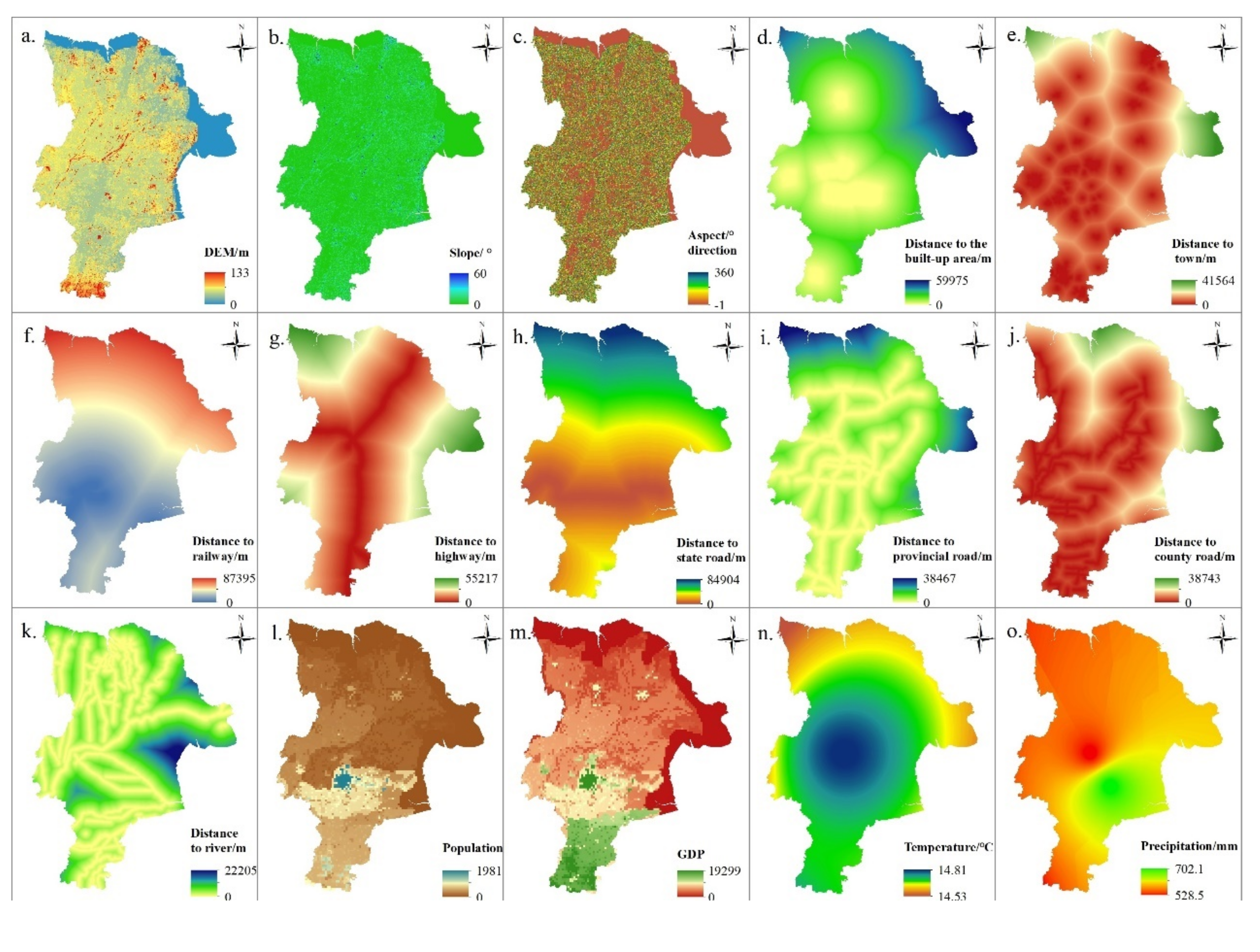
| Terrain factors | DEM | Resource and Environment Science Data Center of Chinese Academy of Sciences (http://www.resdc.cn/) | Resolution: 30 m × 30 m. It derived from SRTM data. The slope and aspect data were calculated using ArcGIS. |
| Slope | |||
| Aspect | |||
| Accessibility | Distance to built-up areas | Geographical Information Monitoring Cloud Platform(http://www.dsac.cn/) | The distance data is calculated using ArcGIS Euclidean distance tool. |
| Distance to town | |||
| Distance to railway | |||
| Distance to highway | |||
| Distance to state road | |||
| Distance to provincial road | |||
| Distance to county road | |||
| Distance to river | |||
| Socioeconomic factors | Population distribution | Resource and Environment Science Data Center of Chinese Academy of Sciences (http://www.resdc.cn/) | We clipped the spatial distribution data of China’s population and GDP. The resolution was converted to 30 m × 30 m from the 1 km precision. |
| GDP distribution | |||
| Climate factors | Annual average temperature | China Meteorological Administration (http://data.cma.cn/) | We used the inverse distance weighted (IDW) interpolation method to spatially interpolate Chinese meteorological data and extracted the meteorological spatial data of Dongying City. |
| Annual average precipitation |
| Scenarios | Name | Parameters and Planning Policy |
|---|---|---|
| S1 | Business as usual (BAU) | The FLUS model parameters remain unchanged, and the area predicted by the Markov chain is used as the land demand data. |
| S2 | Fast cultivated land expansion scenario (FCLE) | Increase the area of cultivated land and decrease the area of construction land, water body, wetland and unused land. Construction land expansion capacity was adjusted to 0.9. |
| S3 | Ecological security scenario (ES) | Increase the area of cultivated land, water body, wetland and unused land, and decrease the area of construction land. The expansion capacity of cultivated land, construction land, forest, water body and wetland were adjusted to 0.2, 0.9, 0.3, 0.2, 0.2, respectively. Ecological redline is used as a restricted area. The conversion cost matrix was changed, see Table 5 for details. |
| S4 | Sustainable development scenario (SD) | Increase the area of cultivated land, forest, water body and wetland, and decrease the area of construction land. The expansion capacity of cultivated land and construction land were adjusted to 0.4 and 0.9. Ecological redline and permanent prime farmland preservation zone were used as restricted areas. The conversion cost matrix is same as S3 (Table 5). |
| Scenarios | Cultivated Land | Garden Land | Forest | Grassland | Construction Land | Water Body | Wetland | Unused Land |
|---|---|---|---|---|---|---|---|---|
| S1 | 215,993 | 4262 | 22,208 | 5487 | 177,100 | 185,178 | 115,601 | 98,814 |
| S2 | 233,273 | 4262 | 22,208 | 5487 | 169,957 | 181,474 | 112,133 | 95,849 |
| S3 | 220,313 | 4262 | 23,512 | 5487 | 159,390 | 187,215 | 116,757 | 107,707 |
| S4 | 225,065 | 4262 | 23,097 | 5487 | 159,390 | 186,420 | 116,179 | 104,743 |
| Scenarios | Cultivated Land | Garden Land | Forest | Grassland | Construction Land | Water Body | Wetland | Unused Land |
|---|---|---|---|---|---|---|---|---|
| S1 | 0.5 | 0.1 | 0.2 | 0.1 | 1 | 0.1 | 0.1 | 0.1 |
| S2 | 0.5 | 0.1 | 0.2 | 0.1 | 0.9 | 0.1 | 0.1 | 0.1 |
| S3 | 0.2 | 0.1 | 0.3 | 0.1 | 0.9 | 0.2 | 0.2 | 0.1 |
| S4 | 0.4 | 0.1 | 0.2 | 0.1 | 0.9 | 0.1 | 0.1 | 0.1 |
| Scenarios | Land Use Type | Cultivated Land | Garden Land | Forest | Grassland | Construction Land | Water Body | Wetland | Unused Land |
|---|---|---|---|---|---|---|---|---|---|
| S1 & S2 | Cultivated land | 1 | 0 | 1 | 0 | 1 | 1 | 0 | 0 |
| Garden land | 1 | 1 | 1 | 0 | 1 | 1 | 0 | 0 | |
| Forest | 1 | 0 | 1 | 0 | 1 | 0 | 0 | 0 | |
| Grassland | 1 | 1 | 1 | 1 | 1 | 1 | 0 | 0 | |
| Construction land | 1 | 1 | 1 | 0 | 1 | 0 | 0 | 0 | |
| Water body | 1 | 1 | 1 | 0 | 1 | 1 | 1 | 0 | |
| Wetland | 1 | 1 | 1 | 1 | 1 | 1 | 1 | 0 | |
| Unused land | 1 | 1 | 1 | 1 | 1 | 1 | 1 | 1 | |
| S3& S4 | Cultivated land | 1 | 0 | 1 | 0 | 1 | 1 | 1 | 0 |
| Garden land | 1 | 1 | 1 | 0 | 1 | 1 | 1 | 0 | |
| Forest | 1 | 0 | 1 | 0 | 1 | 1 | 1 | 0 | |
| Grassland | 1 | 1 | 1 | 1 | 1 | 1 | 1 | 0 | |
| Construction land | 1 | 1 | 1 | 1 | 1 | 0 | 1 | 0 | |
| Water body | 1 | 1 | 1 | 1 | 1 | 1 | 1 | 0 | |
| Wetland | 1 | 1 | 1 | 1 | 1 | 1 | 1 | 0 | |
| Unused land | 1 | 1 | 1 | 1 | 1 | 1 | 1 | 1 |
| Threat Type | Max distance | Weight | Decay |
|---|---|---|---|
| Urban land | 10 | 1 | exponential |
| Rural residential land | 5 | 0.7 | exponential |
| Transportation land | 2 | 0.6 | linear |
| Mining land | 4 | 0.8 | exponential |
| Cultivated land | 1 | 0.5 | exponential |
| Saline alkali land | 1 | 0.6 | exponential |
| Land Use Type | Habitat Suitability | Urban Land | Rural Residential Land | Transportation Land | Mining Land | Cultivated Land | Saline alkali Land |
|---|---|---|---|---|---|---|---|
| Cultivated land | 0.4 | 0.5 | 0.6 | 0.2 | 0.5 | 0.3 | 0.8 |
| Garden land | 0.5 | 0.4 | 0.4 | 0.3 | 0.4 | 0.3 | 0.7 |
| Forest | 0.9 | 0.9 | 0.8 | 0.7 | 0.7 | 0.5 | 0.4 |
| Grassland | 0.7 | 0.7 | 0.4 | 0.6 | 0.6 | 0.4 | 0.3 |
| Construction land | 0 | 0 | 0 | 0 | 0 | 0 | 0 |
| Water body | 0.9 | 0.8 | 0.6 | 0.4 | 0.9 | 0.6 | 0.7 |
| Wetland | 0.7 | 0.8 | 0.6 | 0.4 | 0.9 | 0.7 | 0.7 |
| Unused land | 0.1 | 0.6 | 0.6 | 0.3 | 0.2 | 0 | 0.9 |
| Habitat Quality Grade | Habitat Quality Index | 2017 | S1 | S2 | S3 | S4 |
|---|---|---|---|---|---|---|
| Lower | 0–0.1 | 26.99 | 31.34 | 29.14 | 30.22 | 29.67 |
| Low | 0.1–0.4 | 30.07 | 28.41 | 30.31 | 28.74 | 29.32 |
| Middle | 0.4–0.6 | 9.37 | 1.51 | 1.57 | 1.73 | 1.68 |
| High | 0.6–0.7 | 26.55 | 14.74 | 14.29 | 14.80 | 14.80 |
| Higher | 0.7–1 | 7.03 | 23.99 | 24.70 | 24.51 | 24.53 |
Publisher’s Note: MDPI stays neutral with regard to jurisdictional claims in published maps and institutional affiliations. |
© 2021 by the authors. Licensee MDPI, Basel, Switzerland. This article is an open access article distributed under the terms and conditions of the Creative Commons Attribution (CC BY) license (http://creativecommons.org/licenses/by/4.0/).
Share and Cite
Ding, Q.; Chen, Y.; Bu, L.; Ye, Y. Multi-Scenario Analysis of Habitat Quality in the Yellow River Delta by Coupling FLUS with InVEST Model. Int. J. Environ. Res. Public Health 2021, 18, 2389. https://doi.org/10.3390/ijerph18052389
Ding Q, Chen Y, Bu L, Ye Y. Multi-Scenario Analysis of Habitat Quality in the Yellow River Delta by Coupling FLUS with InVEST Model. International Journal of Environmental Research and Public Health. 2021; 18(5):2389. https://doi.org/10.3390/ijerph18052389
Chicago/Turabian StyleDing, Qinglong, Yang Chen, Lingtong Bu, and Yanmei Ye. 2021. "Multi-Scenario Analysis of Habitat Quality in the Yellow River Delta by Coupling FLUS with InVEST Model" International Journal of Environmental Research and Public Health 18, no. 5: 2389. https://doi.org/10.3390/ijerph18052389
APA StyleDing, Q., Chen, Y., Bu, L., & Ye, Y. (2021). Multi-Scenario Analysis of Habitat Quality in the Yellow River Delta by Coupling FLUS with InVEST Model. International Journal of Environmental Research and Public Health, 18(5), 2389. https://doi.org/10.3390/ijerph18052389