
Research on a Novel Hybrid Decomposition–Ensemble Learning Paradigm Based on VMD and IWOA for PM2.5 Forecasting

Abstract
1. Introduction
2. Related Methodology
2.1. Four Individual Prediction Methods
2.1.1. The Back Propagation Neural Network (BPNN)
2.1.2. The Adaptive Network Based Fuzzy Inference System (ANFIS)
2.1.3. The Fuzzy C-Means Clustering (FCM)
2.1.4. The Group Method of Data Handling (GMDH)
2.2. Variation Mode Decomposition (VMD)
2.3. Optimization Algorithm-IWOA
2.3.1. Overview of the Whale Optimization Algorithm
2.3.2. IWOA
| Algorithm: Improved whale-optimization algorithm (IWOA) |
| Objective: |
| Minimize and maximize the objective function , |
| Parameters: |
| iter-iteration number. |
| Maxiter-the maximum number of iteration. |
| I-a population pop. |
| p-the switch probability |
| 1. /*Initialize a population |
| 2. WHILEiter < Maxiter |
| 3. FORi = 1 to I Update , , l and p |
| 4. IFp > 0.5 |
| 5. IF |
| 6. Update the position of the current solution by Equation (14) |
| 7. ELSE IF |
| 8. Randomly choose a search agent |
| 9. Update the position of the current search agent by Equation (16) |
| 10. END IF |
| 11. ELSE IFp > 0.5 |
| 12. Update the position of the current search by Equation (15) |
| 13. END IF |
| 14. END FOR |
| 15. /*Jump out of local optimum by using chaotic local search. */ |
| 16. Calculate |
| 17. Calculate the next iteration chaotic variable by Equation (16) |
| 18. Transform for the next iteration |
| 19. /*Evaluate replace by if the newly generation is better. */ |
| 20. /*Find the current best solution gbest*/ |
| 21. |
| 22. END WHILE |
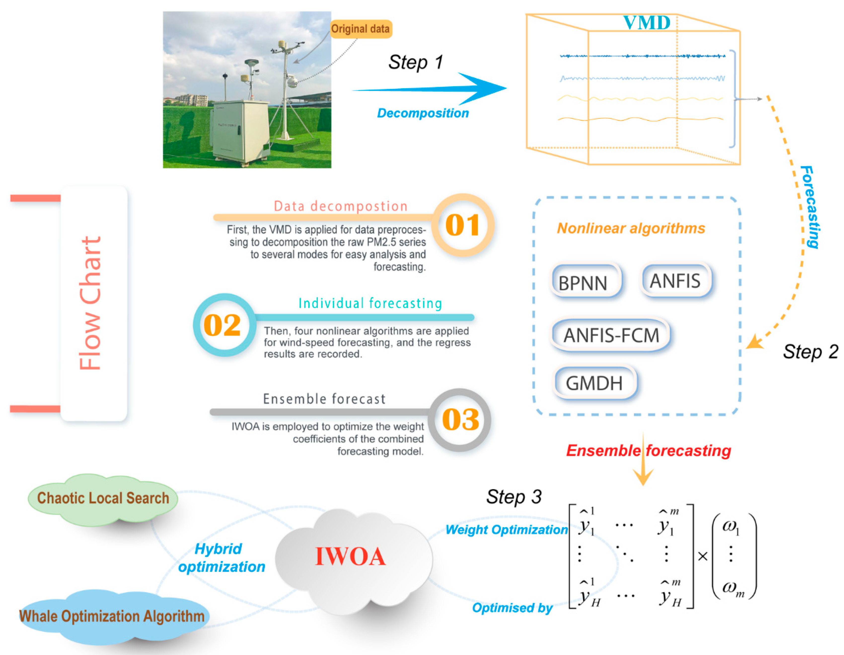
3. Decomposition–Ensemble Learning Paradigm
- -
- Step 1: Decomposition process:
- -
- Step 2: Ensemble forecasting and IWOA optimization:
- -
- Step 3: Assemble forecasting results:
4. Study Areas and the Evaluation Criteria
4.1. Data Description
4.2. Model Assessment Standards
5. Results and Analysis
5.1. Data Decomposition by VMD
5.2. The Process of Ensemble Forecast on VMs
5.3. Model Performance Evaluation and Comparison
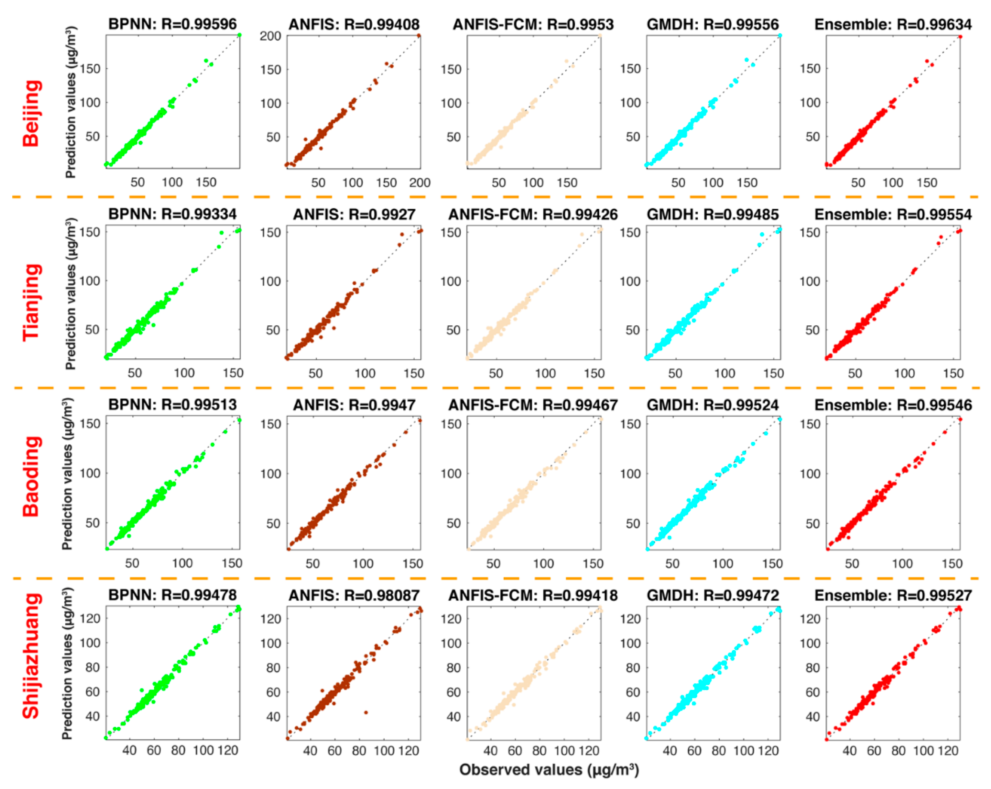
5.3.1. Experiment 1: The Comparison between the Ensemble Model and VMD-Based Models
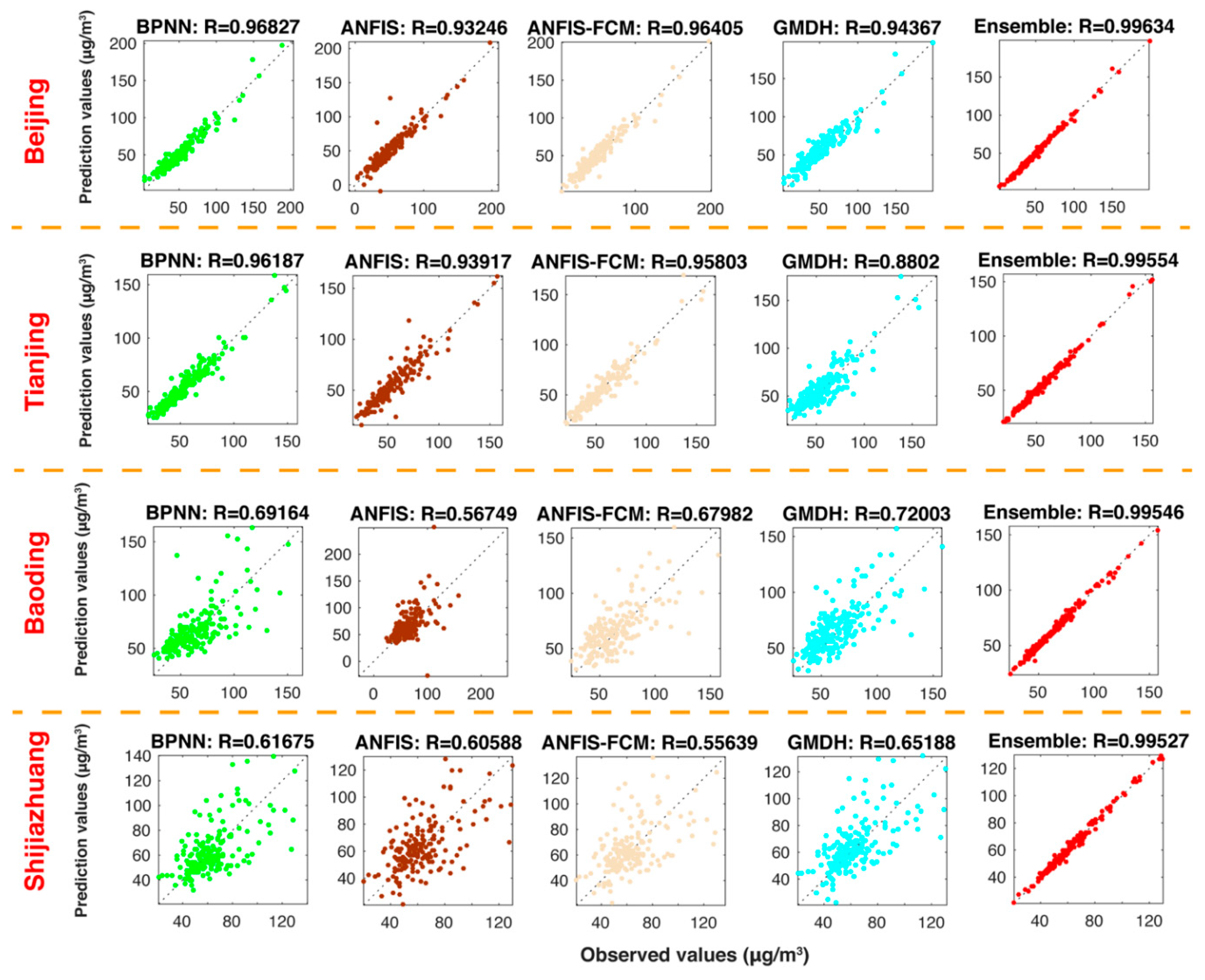
5.3.2. Experiment 2: The Comparison between the Ensemble Model and Individual Models
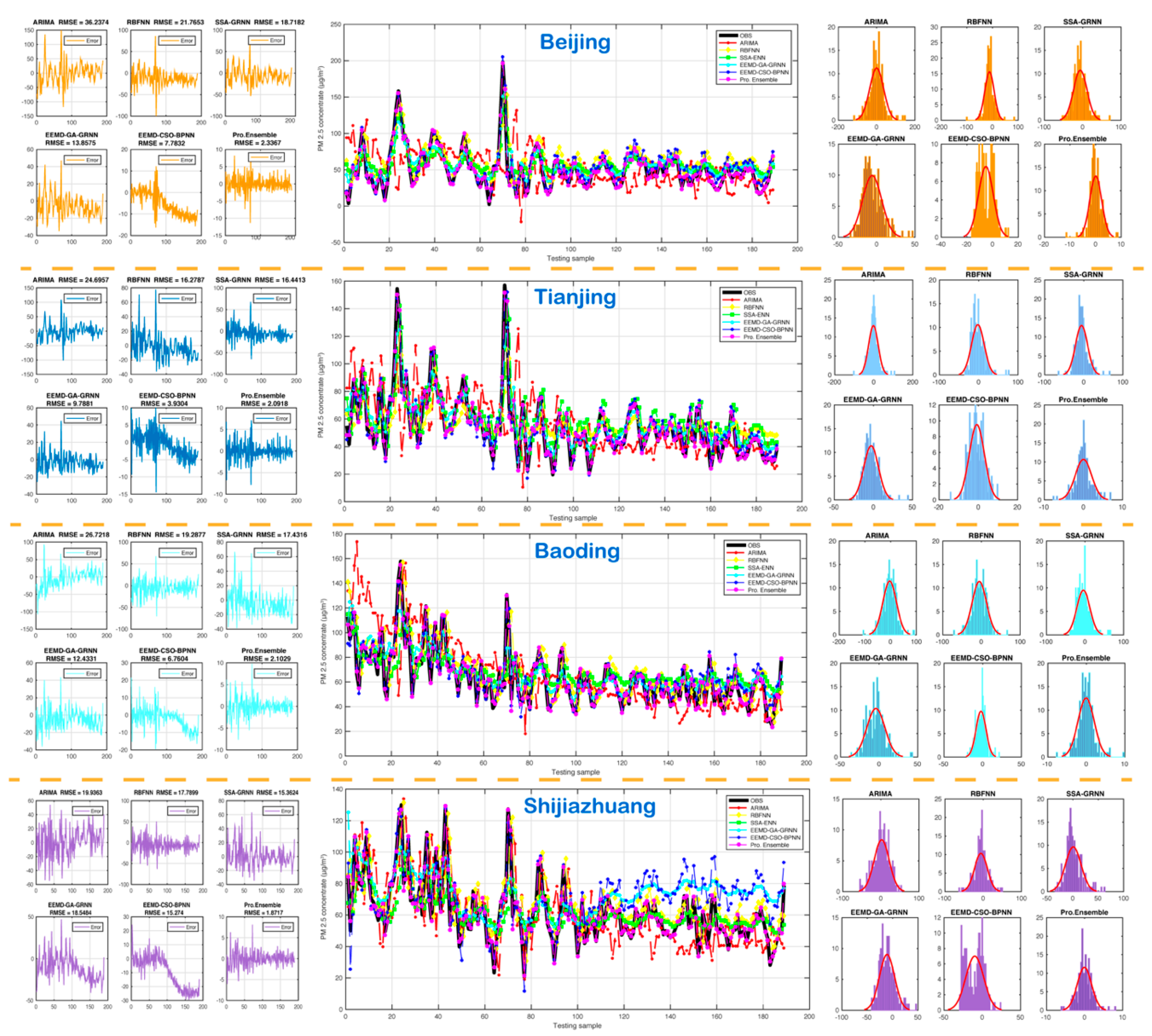
5.3.3. Experiment 3: The Comparison between the Proposed Model and the Existing Models
6. Conclusions
Author Contributions
Funding
Data Availability Statement
Acknowledgments
Conflicts of Interest
References
- Abdoos, A.A. A new intelligent method based on combination of VMD and ELM for short term wind power forecasting. Neurocomputing 2016, 203, 111–120. [Google Scholar] [CrossRef]
- Asadollahfardi, G.; Zangooei, H.; Aria, S.H. Predicting PM2.5 Concentrations Using Artificial Neural Networks and Markov Chain, a Case Study Karaj City. Asian J. Atmos. Environ. 2016, 10, 67–79. [Google Scholar] [CrossRef]
- Elbayoumi, M.; Ramli, N.A.; Yusof, N.F.F.M. Development and comparison of regression models and feedforward backpropagation neural network models to predict seasonal indoor PM2.5–10 and PM2.5 concentrations in naturally ventilated schools. Atmos. Pollut. Res. 2015, 6, 1013–1023. [Google Scholar] [CrossRef]
- Feng, X.; Li, Q.; Zhu, Y.; Hou, J.; Jin, L.; Wang, J. Artificial neural networks forecasting of PM2.5 pollution using air mass trajectory based geographic model and wavelet transformation. Atmos. Environ. 2015, 107, 118–128. [Google Scholar] [CrossRef]
- Fernando, H.; Mammarella, M.; Grandoni, G.; Fedele, P.; Di Marco, R.; Dimitrova, R.; Hyde, P. Forecasting PM10 in metropolitan areas: Efficacy of neural networks. Environ. Pollut. 2012, 163, 62–67. [Google Scholar] [CrossRef]
- Dag, O.; Yozgatligil, C. GMDH: An R Package for Short Term Forecasting via GMDH-Type Neural Network Algorithms. R J. 2016, 8, 379–386. [Google Scholar] [CrossRef]
- Dragomiretskiy, K.; Zosso, D. Variational Mode Decomposition. IEEE Trans. Signal Process. 2014, 62, 531–544. [Google Scholar] [CrossRef]
- Chen, Y.-C.; Lei, T.-C.; Yao, S.; Wang, H.-P. PM2.5 Prediction Model Based on Combinational Hammerstein Recurrent Neural Networks. Mathematics 2020, 8, 2178. [Google Scholar] [CrossRef]
- Wang, X.; Yuan, J.; Wang, B. Prediction and analysis of PM2.5 in Fuling District of Chongqing by artificial neural network. Neural Comput. Appl. 2020, 1–8. [Google Scholar] [CrossRef]
- Jian, L.; Zhao, Y.; Zhu, Y.-P.; Zhang, M.-B.; Bertolatti, D. An application of ARIMA model to predict submicron particle concentrations from meteorological factors at a busy roadside in Hangzhou, China. Sci. Total Environ. 2012, 426, 336–345. [Google Scholar] [CrossRef] [PubMed]
- Konovalov, I.; Beekmann, M.; Meleux, F.; Dutot, A.L.; Foret, G. Combining deterministic and statistical approaches for PM10 forecasting in Europe. Atmos. Environ. 2009, 43, 6425–6434. [Google Scholar] [CrossRef]
- Li, X.; Peng, L.; Yao, X.; Cui, S.; Hu, Y.; You, C.; Chi, T. Long short-term memory neural network for air pollutant concentration predictions: Method development and evaluation. Environ. Pollut. 2017, 231, 997–1004. [Google Scholar] [CrossRef] [PubMed]
- Liu, B.; Wang, L.; Jin, Y.-H.; Tang, F.; Huang, D.-X. Improved particle swarm optimization combined with chaos. Chaos Solitons Fractals 2005, 25, 1261–1271. [Google Scholar] [CrossRef]
- Mirjalili, S.; Lewis, A. The Whale Optimization Algorithm. Adv. Eng. Softw. 2016, 95, 51–67. [Google Scholar] [CrossRef]
- Qiao, W.; Tian, W.; Tian, Y.; Yang, Q.; Zhang, J. The forecasting of PM2.5 using a hybrid model based on wave-let transform and an improved deep learning algorithm. IEEE Access 2019, 7, 142814–142825. [Google Scholar] [CrossRef]
- Liu, H.; Chen, C. Prediction of outdoor PM2.5 concentrations based on a three-stage hybrid neural network model. Atmos. Pollut. Res. 2020, 11, 469–481. [Google Scholar] [CrossRef]
- Wang, D.; Liu, Y.; Luo, H.; Yue, C.; Cheng, S. Day-Ahead PM2.5 Concentration Forecasting Using WT-VMD Based Decomposition Method and Back Propagation Neural Network Improved by Differential Evolution. Int. J. Environ. Res. Public Health 2017, 14, 764. [Google Scholar] [CrossRef] [PubMed]
- Niu, M.; Wang, Y.; Sun, S.; Li, Y. A novel hybrid decomposition-and-ensemble model based on CEEMD and GWO for short-term PM2.5 concentration forecasting. Atmos. Environ. 2016, 134, 168–180. [Google Scholar] [CrossRef]
- Perez, P.; Reyes, J. An integrated neural network model for PM10 forecasting. Atmos. Environ. 2006, 40, 2845–2851. [Google Scholar] [CrossRef]
- Qin, S.; Liu, F.; Wang, J.; Sun, B. Analysis and forecasting of the particulate matter (PM) concentration levels over four major cities of China using hybrid models. Atmos. Environ. 2014, 98, 665–675. [Google Scholar] [CrossRef]
- Qu, Z.; Zhang, W.; Mao, W.; Wang, J.; Liu, C.; Zhang, W. Research and application of ensemble forecasting based on a novel multi-objective optimization algorithm for wind-speed forecasting. Energy Convers. Manag. 2017, 154, 440–454. [Google Scholar] [CrossRef]
- World Health Organization. World Health Statistics; World Health Organization: Geneva, Switzerland, 2011.
- Xiao, L.; Shao, W.; Liang, T.; Wang, C. A combined model based on multiple seasonal patterns and modified firefly algorithm for electrical load forecasting. Appl. Energy 2016, 167, 135–153. [Google Scholar] [CrossRef]
- Xiao, L.; Wang, J.; Dong, Y.; Wu, J. Combined forecasting models for wind energy forecasting: A case study in China. Renew. Sustain. Energy Rev. 2015, 44, 271–288. [Google Scholar] [CrossRef]
- Yang, Y.; Chen, Y.; Wang, Y.; Li, C.; Li, L. Modelling a combined method based on ANFIS and neural network improved by DE algorithm: A case study for short-term electricity demand forecasting. Appl. Soft Comput. 2016, 49, 663–675. [Google Scholar] [CrossRef]
- Zhang, N.; Lin, A.; Shang, P. Multidimensionalk-nearest neighbor model based on EEMD for financial time series forecasting. Phys. A Stat. Mech. Appl. 2017, 477, 161–173. [Google Scholar] [CrossRef]
- Zhou, Q.; Jiang, H.; Wang, J.; Zhou, J. A hybrid model for PM 2.5 forecasting based on ensemble empirical mode decomposition and a general regression neural network. Sci. Total Environ. 2014, 496, 264–274. [Google Scholar] [CrossRef]


| Metric | Equation | Definition |
|---|---|---|
| MAE | The average absolute forecast error of n times forecast results | |
| RMSE | The root mean-square forecast error | |
| MAPE | The average of absolute error | |
| TIC | Theil’s inequality coefficient |
| Model | Experimental Parameters | Default Value |
|---|---|---|
| BPNN | The learning velocity | 0.01 |
| The maximum number of trainings | 1000 | |
| Training requirements precision | 0.00004 | |
| ANFIS | Spread of radial basis functions | 0.5 |
| Training requirements precision | 0.00004 | |
| FCM | The maximum number of trainings | 1000 |
| Spread of radial basis functions | 0.15 | |
| GMDH | Learning rate | 0.1 |
| Training requirements precision | 0.00004 |
| Models | VM1 | VM2 | VM3 | Residual | |||||
|---|---|---|---|---|---|---|---|---|---|
| Weights | RMSE | Weights | RMSE | Weights | RMSE | Weights | RMSE | ||
| Beijing | BPNN | 0.06880 | 0.32695 | 0.40850 | 0.67043 | 1.24076 | 0.81130 | 0.51770 | 1.16300 |
| ANFIS | 0.30331 | 0.30256 | 0.03701 | 0.75516 | −0.10014 | 1.38320 | 0.38167 | 1.17560 | |
| ANFIS-FCM | 0.00617 | 0.30669 | 0.17178 | 0.73279 | 0.18866 | 0.87710 | −0.48722 | 1.43640 | |
| GMDH | 0.63306 | 0.29672 | 0.38893 | 0.68048 | −0.34365 | 0.86398 | 0.56177 | 1.16110 | |
| Ensemble model | - | 0.29096 | - | 0.65445 | - | 0.79141 | - | 1.05820 | |
| Tianjing | BPNN | 0.03703 | 0.31010 | 0.11645 | 0.61997 | 0.16865 | 0.79890 | −0.57673 | 1.34090 |
| ANFIS | 0.34467 | 0.25575 | 0.35167 | 0.64571 | −0.17093 | 0.90740 | −0.00375 | 1.73350 | |
| ANFIS-FCM | 0.26816 | 0.25998 | −0.07272 | 0.66214 | 0.74391 | 0.75810 | −0.14957 | 1.23630 | |
| GMDH | 0.34997 | 0.25685 | 0.61707 | 0.59548 | 0.24071 | 0.78005 | 1.71433 | 0.99831 | |
| Ensemble model | - | 0.24593 | - | 0.57482 | - | 0.73581 | - | 0.93073 | |
| Baoding | BPNN | −0.04298 | 0.36294 | −0.35375 | 0.65537 | 0.11825 | 1.19390 | 0.17385 | 0.82444 |
| ANFIS | 0.72431 | 0.26715 | 0.33840 | 0.67208 | 0.12688 | 1.49690 | 0.40790 | 0.80775 | |
| ANFIS-FCM | 0.10233 | 0.28678 | 0.33900 | 0.65961 | −0.03061 | 1.35590 | −0.00282 | 0.85015 | |
| GMDH | 0.21607 | 0.27619 | 0.67852 | 0.65221 | 0.81967 | 1.13750 | 0.38544 | 0.86024 | |
| Ensemble model | - | 0.26360 | - | 0.63175 | - | 1.08830 | - | 0.77429 | |
| Shijiazhuang | BPNN | −0.07031 | 0.29393 | −1.28208 | 0.60497 | 0.40346 | 1.09080 | −0.01858 | 0.78471 |
| ANFIS | 1.01576 | 0.23183 | 0.50000 | 0.61216 | −0.04074 | 2.99250 | −0.07890 | 0.92644 | |
| ANFIS-FCM | −0.08646 | 0.25504 | −0.20145 | 0.63428 | 0.15397 | 1.18430 | 0.32321 | 0.78460 | |
| GMDH | 0.14144 | 0.23988 | 2.00000 | 0.57380 | 0.50412 | 1.06280 | 0.75931 | 0.72264 | |
| Ensemble model | - | 0.22918 | - | 0.55405 | - | 1.01030 | - | 0.70881 | |
| Dataset | Indicator | Ensemble Model vs. VMD-BPNN | Ensemble Model vs. VMD-ANFIS | Ensemble Model vs. VMD-ANFIS-FCM | Ensemble Model vs. VMD-GMDH |
|---|---|---|---|---|---|
| Beijing | IMAE (%) | 2.3843 | 10.6660 | 3.6867 | 2.1953 |
| IRMSE (%) | 5.4454 | 21.3895 | 11.6926 | 9.7510 | |
| IMAPE (%) | 0.3159 | 11.9748 | 12.3061 | 5.3553 | |
| ITIC (%) | 5.2795 | 21.3508 | 11.6465 | 9.6318 | |
| Tianjing | IMAE (%) | 14.0270 | 14.5473 | 7.3431 | 3.5937 |
| IRMSE (%) | 18.0484 | 21.9939 | 11.8452 | 7.1982 | |
| IMAPE (%) | 14.5592 | 12.9259 | 10.8481 | 3.3801 | |
| ITIC (%) | 18.0279 | 22.0097 | 11.7854 | 7.1898 | |
| Baoding | IMAE (%) | 2.8295 | 7.3044 | 6.9863 | 0.5752 |
| IRMSE (%) | 3.9004 | 7.4784 | 7.6538 | 2.3325 | |
| IMAPE (%) | 2.1528 | 7.0565 | 6.0185 | 0.0488 | |
| ITIC (%) | 3.8167 | 7.5020 | 7.6881 | 2.3468 | |
| Shijiazhuang | IMAE (%) | 1.4251 | 18.7068 | 4.7226 | 4.8292 |
| IRMSE (%) | 4.8678 | 49.9864 | 9.2788 | 5.0535 | |
| IMAPE (%) | 1.2716 | 15.5030 | 5.3138 | 4.0961 | |
| ITIC (%) | 4.8218 | 50.0715 | 9.3976 | 5.0563 |
| Dataset | Indicator | Ensemble Model vs. BPNN | Ensemble Model vs. ANFIS | Ensemble Model vs. ANFIS-FCM | Ensemble Model vs. GMDH |
|---|---|---|---|---|---|
| Beijing | IMAE (%) | 68.6537 | 71.9248 | 69.1895 | 80.9890 |
| IRMSE (%) | 66.6395 | 76.9644 | 68.1596 | 78.5772 | |
| IMAPE (%) | 69.6792 | 68.0098 | 58.9320 | 79.7105 | |
| ITIC (%) | 66.3829 | 76.7079 | 67.9496 | 77.7231 | |
| Tianjing | IMAE (%) | 66.4829 | 71.3965 | 67.8848 | 82.5946 |
| IRMSE (%) | 65.7865 | 73.3943 | 67.7401 | 81.1458 | |
| IMAPE (%) | 67.7547 | 71.7270 | 67.5358 | 83.5715 | |
| ITIC (%) | 65.6355 | 73.1804 | 67.5553 | 80.7598 | |
| Baoding | IMAE (%) | 87.9473 | 90.1459 | 89.0888 | 88.2149 |
| IRMSE (%) | 88.0371 | 90.9558 | 88.0382 | 87.3972 | |
| IMAPE (%) | 88.0240 | 89.6555 | 89.2647 | 88.3508 | |
| ITIC (%) | 87.7416 | 90.6394 | 87.7908 | 87.0859 | |
| Shijiazhuang | IMAE (%) | 88.3384 | 88.7396 | 89.1616 | 88.0327 |
| IRMSE (%) | 88.8181 | 88.9320 | 89.5788 | 88.2980 | |
| IMAPE (%) | 87.7574 | 88.4450 | 88.8123 | 87.8461 | |
| ITIC (%) | 88.8018 | 88.8921 | 89.4880 | 88.1406 |
| Dataset | Indicator | MAE | RMSE | MAPE | TIC | Error Mean | Error STD |
|---|---|---|---|---|---|---|---|
| Beijing | ARIMA | 26.4865 | 36.2374 | 92.8296 | 0.3176 | −0.1317 | 36.3334 |
| RBFNN | 17.0813 | 21.7653 | 62.7264 | 0.1751 | −11.9703 | 18.2263 | |
| SSA-ENN | 14.8237 | 18.7182 | 56.8534 | 0.1593 | −6.4266 | 17.6271 | |
| EEMD-GRNN | 11.3569 | 13.8575 | 41.9101 | 0.1176 | −6.0212 | 12.5142 | |
| EEMD-WOA-BPNN | 6.3748 | 7.7832 | 18.0544 | 0.0647 | −5.2481 | 5.7629 | |
| Pro. Ensemble | 1.6843 | 2.3367 | 5.5600 | 0.0202 | 0.0577 | 2.3422 | |
| Tianjing | ARIMA | 17.4613 | 24.6957 | 35.4034 | 0.2059 | −1.6273 | 24.7075 |
| RBFNN | 12.5062 | 16.2787 | 26.4680 | 0.1376 | −2.2933 | 16.1591 | |
| SSA-ENN | 12.4636 | 16.4413 | 26.2710 | 0.1335 | −5.6593 | 15.4776 | |
| EEMD-GRNN | 7.6808 | 9.7881 | 16.3186 | 0.0815 | −2.8509 | 9.3886 | |
| EEMD-WOA-BPNN | 3.2047 | 3.9304 | 6.6289 | 0.0328 | −0.8012 | 3.8581 | |
| Pro. Ensemble | 1.4745 | 2.0918 | 2.7869 | 0.0176 | 0.0061 | 2.0973 | |
| Baoding | ARIMA | 20.0634 | 26.7218 | 31.9956 | 0.1888 | −3.9880 | 26.4927 |
| RBFNN | 15.0370 | 19.2877 | 25.5808 | 0.1376 | −5.4023 | 18.5648 | |
| SSA-ENN | 13.4114 | 17.4316 | 24.1157 | 0.1275 | −4.2010 | 16.9627 | |
| EEMD-GRNN | 9.5818 | 12.4331 | 17.2851 | 0.0902 | −4.2821 | 11.7035 | |
| EEMD-WOA-BPNN | 5.0988 | 6.7604 | 9.2280 | 0.0495 | −2.2183 | 6.4030 | |
| Pro. Ensemble | 1.4926 | 2.1029 | 2.4427 | 0.0156 | −0.0498 | 2.1079 | |
| Shijiazhuang | ARIMA | 15.5991 | 19.9363 | 25.4303 | 0.1541 | 1.9553 | 19.8929 |
| RBFNN | 13.4980 | 17.7899 | 23.6275 | 0.1310 | −5.9717 | 16.8022 | |
| SSA-ENN | 11.1319 | 15.3624 | 18.5469 | 0.1204 | 0.9266 | 15.3752 | |
| EEMD-GRNN | 15.5582 | 18.5484 | 29.2907 | 0.1326 | −11.1552 | 14.8584 | |
| EEMD-WOA-BPNN | 11.9964 | 15.2740 | 22.6224 | 0.1093 | −9.8333 | 11.7187 | |
| Pro. Ensemble | 1.4004 | 1.8717 | 2.3930 | 0.0143 | −0.0449 | 1.8762 |
Publisher’s Note: MDPI stays neutral with regard to jurisdictional claims in published maps and institutional affiliations. |
© 2021 by the authors. Licensee MDPI, Basel, Switzerland. This article is an open access article distributed under the terms and conditions of the Creative Commons Attribution (CC BY) license (http://creativecommons.org/licenses/by/4.0/).
Share and Cite
Guo, H.; Guo, Y.; Zhang, W.; He, X.; Qu, Z. Research on a Novel Hybrid Decomposition–Ensemble Learning Paradigm Based on VMD and IWOA for PM2.5 Forecasting. Int. J. Environ. Res. Public Health 2021, 18, 1024. https://doi.org/10.3390/ijerph18031024
Guo H, Guo Y, Zhang W, He X, Qu Z. Research on a Novel Hybrid Decomposition–Ensemble Learning Paradigm Based on VMD and IWOA for PM2.5 Forecasting. International Journal of Environmental Research and Public Health. 2021; 18(3):1024. https://doi.org/10.3390/ijerph18031024
Chicago/Turabian StyleGuo, Hengliang, Yanling Guo, Wenyu Zhang, Xiaohui He, and Zongxi Qu. 2021. "Research on a Novel Hybrid Decomposition–Ensemble Learning Paradigm Based on VMD and IWOA for PM2.5 Forecasting" International Journal of Environmental Research and Public Health 18, no. 3: 1024. https://doi.org/10.3390/ijerph18031024
APA StyleGuo, H., Guo, Y., Zhang, W., He, X., & Qu, Z. (2021). Research on a Novel Hybrid Decomposition–Ensemble Learning Paradigm Based on VMD and IWOA for PM2.5 Forecasting. International Journal of Environmental Research and Public Health, 18(3), 1024. https://doi.org/10.3390/ijerph18031024