
Performance of a Genetic Algorithm for Estimating DeGroot Opinion Diffusion Model Parameters for Health Behavior Interventions


Abstract
:1. Introduction
2. Materials and Methods
2.1. Modeling Opinion Diffusion
2.1.1. DeGroot Model
2.1.2. Transformations
Forward Transformation:
- Begin with data on an n-point ordinal scale, converting to a 1 to n scale if necessary.
- Divide the interval into n sub-intervals of equal width.
- An opinion of x on the ordinal scale takes on the middle value, y, in the xth sub-interval on the continuous scale.
Back Transformation:
- Begin with data on a continuous interval to be converted to an n-point ordinal scale.
- Multiply the continuous opinion y by n.
- Round the multiplied continuous opinion up to an integer (ceiling function) to produce an opinion on the ordinal scale. (This final step does not work for the edge case where , so any such values are automatically converted to an ordinal value of 1.)
2.1.3. Objective Function
2.1.4. Genetic Algorithm
2.2. PrEP Pilot Study
2.2.1. Motivation
2.2.2. Network Recruitment
2.2.3. Intervention and Data Collection
2.2.4. Measures
2.2.5. Limitations
2.3. Simulation Study
2.3.1. Ordinal Data
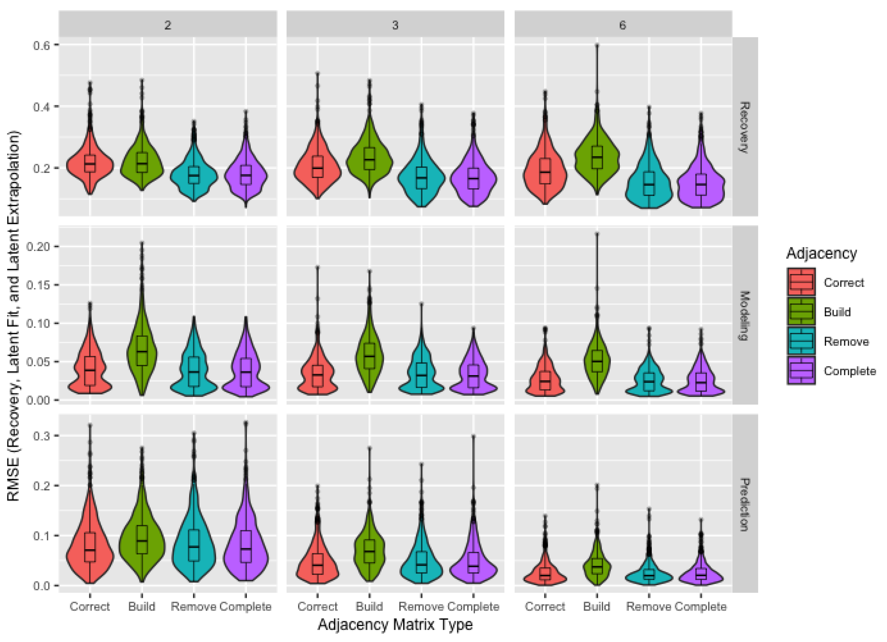
2.3.2. Adjacency Matrix
- Missing Agents: Since this study uses two waves, agents with a geodesic distance to the seed larger than two—those who are friends of friends of friends of the seed or further removed—are always excluded from the sample. Additionally, some nominated agents may decline to participate, with 53% of the individuals named during the recruitment process agreeing to participate in the PrEP pilot study. We consider both the possibility of guaranteed recruitment () and non-guaranteed recruitment (), informed by the recruitment percentage in the pilot study.
- Unknown Links: While we have described situations where the presence or absence of a link in the network is unknown, the adjacency matrix does not have the flexibility to indicate an unknown link, requiring us to specify either the presence () or absence () of a link between agents i and j. When information about all nominations—including repeats—is available, we know all links between the sampled agents. We refer to the adjacency matrix where all links between sampled agents are known as the correct matrix. Note that “correct” refers only to the links between sampled agents and does not imply all agents in the true network are included in the sample. Unfortunately, it is usually impractical or unethical to obtain the information necessary for the correct matrix. We include it in the simulation study, not as a viable solution to the issue of missing links, but as a baseline for comparison for more practical solutions and to determine the consequences of failing to collect the information necessary for the correct matrix.
2.3.3. Model Misspecification
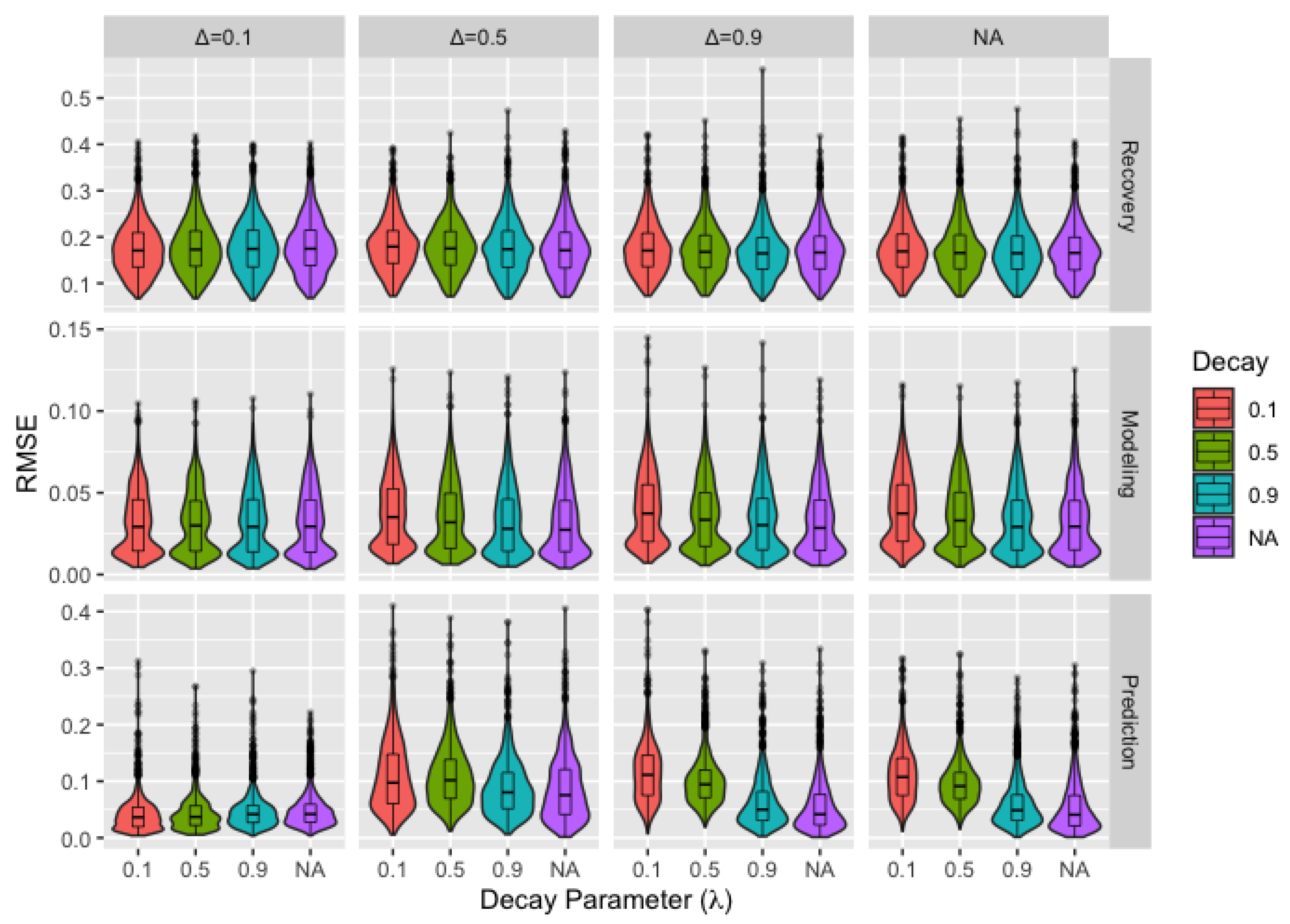
- Bounded Confidence: For bounded confidence, we assume agents with sufficiently differing opinions will either not discuss the topic or will be otherwise unable to influence each other. This is accomplished through the addition of the restriction on the weight matrix Wwhere represents the maximum difference between opinions after which agents are unable to influence each other [32]. This is equivalent to the DeGroot model when . Since changing opinions allow for agents falling within the threshold for bounded confidence at some time steps and not at others, the application of bounded confidence necessitates a notation adjustment. We define W as the weight matrix in the absence of bounded confidence restrictions and as the weight matrix after applying the appropriate bounded confidence adjustments at time t. Based on this new notation, we update to
- Decay: The second extension of the model allows for agents to place changing weight on their own current opinion according towhere I is an identity matrix and is a scalar adjustment factor allowed to vary with time [32]. The effect of the adjustment is to shift the weight for each agent to (or from, depending on the values of ) their self-weight. In order for such a model to be useful, we impose a structure: setting equal to to the power of t, so that agents place decaying weight on the opinions of others. We modify the previous equation towith . Equation (5b) is equivalent to the DeGroot model if . Given the structure imposed on , these models result in an opinion diffusion process where agents place progressively more weight on their own opinions over time, resulting in more confident or stubborn agents whose opinions change less with each time step. This effect is most pronounced when is further from one, so we consider data generated under decay models with decay parameter of 0.1, 0.5, and 0.9.
2.3.4. Procedure
2.3.5. Performance Metrics
3. Results
3.1. Network Sampling
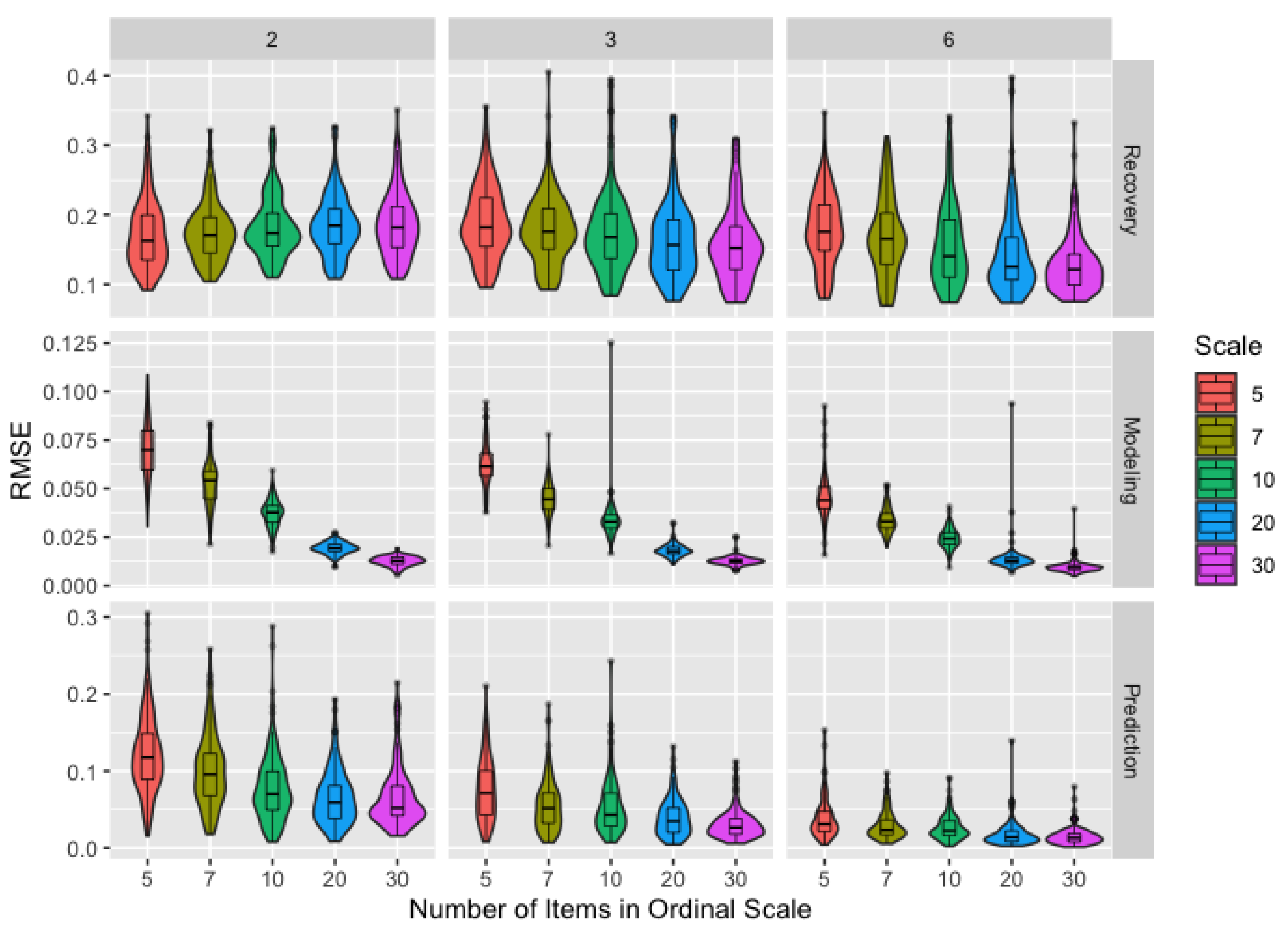
3.2. Ordinal Data
3.3. Alternate Models
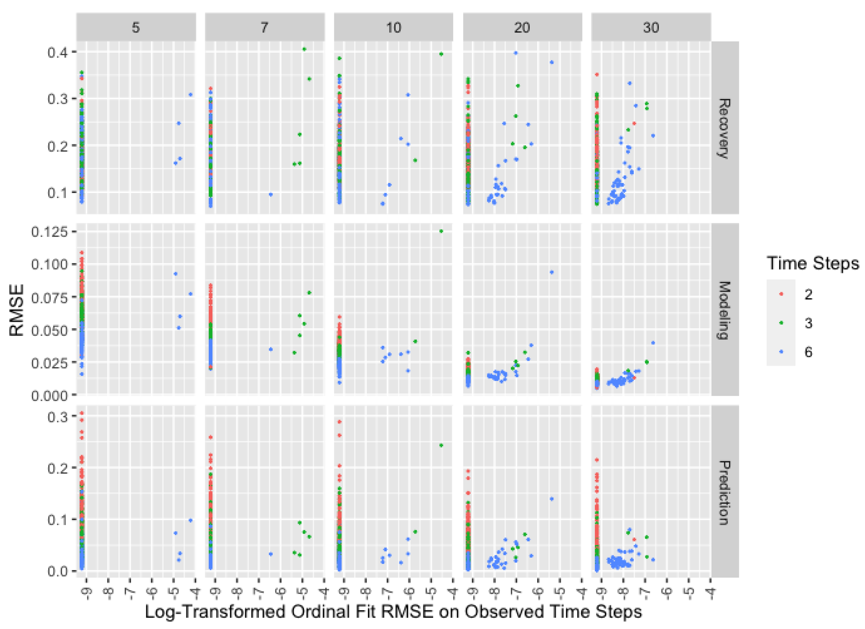
3.4. Performance Diagnostics
4. Discussion
5. Conclusions
Author Contributions
Funding
Institutional Review Board Statement
Informed Consent Statement
Data Availability Statement
Acknowledgments
Conflicts of Interest
Abbreviations
| PrEP | pre-exposure prophylaxis |
| BMSM | Black men who have sex with men |
| MSM | men who have sex with men |
| HIV | human immunodeficiency virus |
| LGBT | lesbian, gay, bisexual, and transgender |
| RMSE | root-mean-square error |
References
- Kelly, J.A.; Amirkhanian, Y.A.; Walsh, J.L.; Brown, K.D.; Quinn, K.G.; Petroll, A.E.; Pearson, B.M.; Rosado, A.N.; Ertl, T. Social network intervention to increase pre-exposure prophylaxis (PrEP) awareness, interest, and use among African American men who have sex with men. AIDS Care 2020, 32, 40–46. [Google Scholar] [CrossRef]
- Johnson, K.L.; Walsh, J.L.; Amirkhanian, Y.A.; Borkowski, J.J.; Carnegie, N.B. Using a novel genetic algorithm to assess peer influence on willingness to use pre-exposure prophylaxis in networks of Black men who have sex with men. Appl. Netw. Sci. 2021, 6, 22. [Google Scholar] [CrossRef]
- O’Connell, A.A. Methods for modeling ordinal outcome variables. Meas. Eval. Couns. Dev. 2000, 33, 170–193. [Google Scholar] [CrossRef]
- DeGroot, M.H. Reaching a consensus. J. Am. Stat. Assoc. 1974, 69, 118–121. [Google Scholar] [CrossRef]
- Acemoglu, D.; Ozdaglar, A. Opinion dynamics and learning in social networks. Dyn. Games Appl. 2011, 1, 3–49. [Google Scholar] [CrossRef]
- Chandrasekhar, A.G.; Larreguy, H.; Xandri, J.P. Testing models of social learning on networks: Evidence from two experiments. Econometrica 2020, 88, 1–32. [Google Scholar] [CrossRef] [Green Version]
- Grimm, V.; Mengel, F. Experiments on belief formation in networks. J. Eur. Econ. Assoc. 2020, 18, 49–82. [Google Scholar] [CrossRef]
- Bezanson, J.; Edelman, A.; Karpinski, S.; Shah, V.B. Julia: A fresh approach to numerical computing. SIAM Rev. 2017, 59, 65–98. [Google Scholar] [CrossRef] [Green Version]
- Schneider, J.A.; Bouris, A.; Smith, D.K. Race and the public health impact potential of pre-exposure prophylaxis in the United States. JAIDS J. Acquir. Immune Defic. Syndr. 2015, 70, e30–e32. [Google Scholar] [CrossRef]
- Paltiel, A.D.; Freedberg, K.A.; Scott, C.A.; Schackman, B.R.; Losina, E.; Wang, B.; Seage, G.R.; Sloan, C.E.; Sax, P.E.; Walensky, R.P. HIV preexposure prophylaxis in the United States: Impact on lifetime infection risk, clinical outcomes, and cost-effectiveness. Clin. Infect. Dis. 2009, 48, 806–815. [Google Scholar] [CrossRef] [Green Version]
- Golub, S.A.; Gamarel, K.E.; Surace, A. Demographic differences in PrEP-related stereotypes: Implications for implementation. AIDS Behav. 2017, 21, 1229–1235. [Google Scholar] [CrossRef]
- Hernández-Romieu, A.C.; Sullivan, P.S.; Rothenberg, R.; Grey, J.; Luisi, N.; Kelley, C.F.; Rosenberg, E.S. Heterogeneity of HIV prevalence among the sexual networks of Black and White MSM in Atlanta: Illuminating a mechanism for increased HIV risk for young Black MSM. Sex. Transm. Dis. 2015, 42, 505. [Google Scholar] [CrossRef] [Green Version]
- Latkin, C.; Donnell, D.; Liu, T.Y.; Davey-Rothwell, M.; Celentano, D.; Metzger, D. The dynamic relationship between social norms and behaviors: The results of an HIV prevention network intervention for injection drug users. Addiction 2013, 108, 934–943. [Google Scholar] [CrossRef] [Green Version]
- Amirkhanian, Y.A.; Kelly, J.A.; Kabakchieva, E.; Kirsanova, A.V.; Vassileva, S.; Takacs, J.; DiFranceisco, W.J.; McAuliffe, T.L.; Khoursine, R.A.; Mocsonaki, L. A randomized social network HIV prevention trial with young men who have sex with men in Russia and Bulgaria. AIDS 2005, 19, 1897–1905. [Google Scholar] [CrossRef]
- Amirkhanian, Y.A.; Kelly, J.A.; Takacs, J.; McAuliffe, T.L.; Kuznetsova, A.V.; Toth, T.P.; Mocsonaki, L.; DiFranceisco, W.J.; Meylakhs, A. Effects of a social network HIV/STD prevention intervention for men who have sex with men in Russia and Hungary: A randomized controlled trial. AIDS 2015, 29, 583. [Google Scholar] [CrossRef] [Green Version]
- Dickson-Gomez, J.; Owczarzak, J.; Lawrence, J.S.; Sitzler, C.; Quinn, K.; Pearson, B.; Kelly, J.A.; Amirkhanian, Y.A. Beyond the ball: Implications for HIV risk and prevention among the constructed families of African American men who have sex with men. AIDS Behav. 2014, 18, 2156–2168. [Google Scholar] [CrossRef] [Green Version]
- Rodgers, E.M. Diffusion of Innovations, 3rd ed.; Free Press: New York, NY, USA, 1983. [Google Scholar]
- Ajzen, I. The theory of planned behavior. Organ. Behav. Hum. Decis. Process. 1991, 50, 179–211. [Google Scholar] [CrossRef]
- Fisher, J.D.; Fisher, W.A. The information-motivation-behavioral skills model. Emerg. Theor. Health Promot. Pract. Res. Strateg. Improv. Public Health 2002, 1, 40–70. [Google Scholar]
- Holden, G. The relationship of self-efficacy appraisals to subsequent health related outcomes: A meta-analysis. Soc. Work Health Care 1992, 16, 53–93. [Google Scholar] [CrossRef]
- Sheeran, P.; Maki, A.; Montanaro, E.; Avishai-Yitshak, A.; Bryan, A.; Klein, W.M.; Miles, E.; Rothman, A.J. The impact of changing attitudes, norms, and self-efficacy on health-related intentions and behavior: A meta-analysis. Health Psychol. 2016, 35, 1178. [Google Scholar] [CrossRef]
- Walsh, J.L. Applying the information–motivation–behavioral skills model to understand PrEP intentions and use among men who have sex with men. AIDS Behav. 2019, 23, 1904–1916. [Google Scholar] [CrossRef]
- Serota, D.P.; Rosenberg, E.S.; Sullivan, P.S.; Thorne, A.L.; Rolle, C.P.M.; Del Rio, C.; Cutro, S.; Luisi, N.; Siegler, A.J.; Sanchez, T.H.; et al. Pre-exposure prophylaxis uptake and discontinuation among young black men who have sex with men in Atlanta, Georgia: A prospective cohort study. Clin. Infect. Dis. 2020, 71, 574–582. [Google Scholar] [CrossRef]
- Golub, S.A.; Fikslin, R.A.; Goldberg, M.H.; Peña, S.M.; Radix, A. Predictors of PrEP uptake among patients with equivalent access. AIDS Behav. 2019, 23, 1917–1924. [Google Scholar] [CrossRef]
- Shrestha, R.; Altice, F.L.; Huedo-Medina, T.B.; Karki, P.; Copenhaver, M. Willingness to use pre-exposure prophylaxis (PrEP): An empirical test of the information-motivation-behavioral skills (IMB) model among high-risk drug users in treatment. AIDS Behav. 2017, 21, 1299. [Google Scholar] [CrossRef] [PubMed] [Green Version]
- Hoots, B.E.; Finlayson, T.; Nerlander, L.; Paz-Bailey, G.; National HIV Behavioral Surveillance Study Group; Wortley, P.; Todd, J.; Sato, K.; Flynn, C.; German, D.; et al. Willingness to take, use of, and indications for pre-exposure prophylaxis among men who have sex with men—20 US cities, 2014. Clin. Infect. Dis. 2016, 63, 672–677. [Google Scholar] [CrossRef] [Green Version]
- Eaton, L.A.; Driffin, D.D.; Smith, H.; Conway-Washington, C.; White, D.; Cherry, C. Psychosocial factors related to willingness to use pre-exposure prophylaxis for HIV prevention among Black men who have sex with men attending a community event. Sex. Health 2014, 11, 244–251. [Google Scholar] [CrossRef]
- Holloway, I.W.; Tan, D.; Gildner, J.L.; Beougher, S.C.; Pulsipher, C.; Montoya, J.A.; Plant, A.; Leibowitz, A. Facilitators and barriers to pre-exposure prophylaxis willingness among young men who have sex with men who use geosocial networking applications in California. AIDS Patient Care STDs 2017, 31, 517–527. [Google Scholar] [CrossRef]
- Patrick, R.; Forrest, D.; Cardenas, G.; Opoku, J.; Magnus, M.; Phillips, G., 2nd; Greenberg, A.; Metsch, L.; Kharfen, M.; LaLota, M.; et al. Awareness, willingness, and use of pre-exposure prophylaxis among men who have sex with men in Washington, DC and Miami-Dade County, FL: National HIV behavioral surveillance, 2011 and 2014. J. Acquir. Immune Defic. Syndr. (1999) 2017, 75, S375. [Google Scholar] [CrossRef]
- Gibbons, F.X.; Gerrard, M.; Ouellette, J.A.; Burzette, R. Cognitive antecedents to adolescent health risk: Discriminating between behavioral intention and behavioral willingness. Psychol. Health 1998, 13, 319–339. [Google Scholar] [CrossRef]
- Gibbons, F.X.; Gerrard, M.; Blanton, H.; Russell, D.W. Reasoned action and social reaction: Willingness and intention as independent predictors of health risk. J. Personal. Soc. Psychol. 1998, 74, 1164. [Google Scholar] [CrossRef]
- Jackson, M.O. Social and Economic Networks; Princeton University Press: Princeton, NJ, USA, 2010. [Google Scholar]

| Input | Values | Notes |
|---|---|---|
| Network Size | Reachability enforced | |
| Degree | Minimum degree for all nodes | |
| Self-Weight | Beta Distribution with | |
| Time Steps | Performance assessed on | |
| Scale | ||
| Recruitment Probability | ||
| Adjacency Matrix | correct, build, remove, complete | |
| Bounded Confidence | equivalent to DeGroot model | |
| Decay | equivalent to DeGroot model |
| Willingness | ||||||||
|---|---|---|---|---|---|---|---|---|
| Build | Remove | |||||||
| Eli | 0.50 | 0.50 | 0.00 | 0.00 | 0.48 | 0.52 | 0.00 | 0.00 |
| Jay | 0.49 | 0.51 | 0 | 0 | 0.53 | 0.47 | 0.00 | 0.00 |
| Uba | 0.04 | 0 | 0.96 | 0 | 0.00 | 0.00 | 0.68 | 0.32 |
| Max | 0.21 | 0 | 0 | 0.79 | 0.12 | 0.09 | 0.00 | 0.79 |
| Eli | Jay | Uba | Max | Eli | Jay | Uba | Max | |
| Self-Efficacy | ||||||||
|---|---|---|---|---|---|---|---|---|
| Build | Remove | |||||||
| Eli | 0.71 | 0.00 | 0.00 | 0.29 | 0.71 | 0.00 | 0.00 | 0.29 |
| Jay | 0.12 | 0.88 | 0 | 0 | 0.10 | 0.88 | 0.00 | 0.02 |
| Uba | 0.00 | 0 | 1.00 | 0 | 0.00 | 0.00 | 1.00 | 0.00 |
| Max | 0.00 | 0 | 0 | 1.00 | 0.00 | 0.00 | 0.00 | 1.00 |
| Eli | Jay | Uba | Max | Eli | Jay | Uba | Max | |
| Network | Willingness | Self-Efficacy | ||||
|---|---|---|---|---|---|---|
| Leader | Non-Leader | Difference | Leader | Non-Leader | Difference | |
| 1 | 0.11 | 0.05 | 0.06 | 0.04 | 0.05 | −0.01 |
| 2 | 0.09 | 0.08 | 0.01 | 0.04 | 0.09 | −0.05 |
| 3 | 0.25 | 0.11 | 0.14 | 0.02 | 0.07 | −0.05 |
| 4 | 0.02 | 0.13 | −0.11 | 0.30 | 0.05 | 0.25 |
| 5 | 0.21 | 0.05 | 0.16 | 0.02 | 0.05 | −0.03 |
| Willingness | Self-Efficacy | |||||||||
|---|---|---|---|---|---|---|---|---|---|---|
| Seed | 0.40 | 0.01 | 0.57 | 0.02 | 0 | 0.72 | 0.08 | 0.15 | 0.04 | 0 |
| Cam | 0.18 | 0.70 | 0.06 | 0.01 | 0.04 | 0.00 | 0.70 | 0.00 | 0.25 | 0.05 |
| Obe | 0.00 | 0.00 | 0.99 | 0.00 | 0.00 | 0.01 | 0.00 | 0.99 | 0.00 | 0.00 |
| Leader | 0.00 | 0.32 | 0.00 | 0.68 | 0.00 | 0.00 | 0.00 | 0.00 | 1.00 | 0.00 |
| Ray | 0 | 0.01 | 0.61 | 0.03 | 0.35 | 0 | 0.00 | 0.07 | 0.91 | 0.02 |
| Seed | Cam | Obe | Leader | Ray | Seed | Cam | Obe | Leader | Ray | |
Publisher’s Note: MDPI stays neutral with regard to jurisdictional claims in published maps and institutional affiliations. |
© 2021 by the authors. Licensee MDPI, Basel, Switzerland. This article is an open access article distributed under the terms and conditions of the Creative Commons Attribution (CC BY) license (https://creativecommons.org/licenses/by/4.0/).
Share and Cite
Johnson, K.L.; Walsh, J.L.; Amirkhanian, Y.A.; Carnegie, N.B. Performance of a Genetic Algorithm for Estimating DeGroot Opinion Diffusion Model Parameters for Health Behavior Interventions. Int. J. Environ. Res. Public Health 2021, 18, 13394. https://doi.org/10.3390/ijerph182413394
Johnson KL, Walsh JL, Amirkhanian YA, Carnegie NB. Performance of a Genetic Algorithm for Estimating DeGroot Opinion Diffusion Model Parameters for Health Behavior Interventions. International Journal of Environmental Research and Public Health. 2021; 18(24):13394. https://doi.org/10.3390/ijerph182413394
Chicago/Turabian StyleJohnson, Kara Layne, Jennifer L. Walsh, Yuri A. Amirkhanian, and Nicole Bohme Carnegie. 2021. "Performance of a Genetic Algorithm for Estimating DeGroot Opinion Diffusion Model Parameters for Health Behavior Interventions" International Journal of Environmental Research and Public Health 18, no. 24: 13394. https://doi.org/10.3390/ijerph182413394
APA StyleJohnson, K. L., Walsh, J. L., Amirkhanian, Y. A., & Carnegie, N. B. (2021). Performance of a Genetic Algorithm for Estimating DeGroot Opinion Diffusion Model Parameters for Health Behavior Interventions. International Journal of Environmental Research and Public Health, 18(24), 13394. https://doi.org/10.3390/ijerph182413394