Article

Prediction of Geosmin at Different Depths of Lake Using Machine Learning Techniques

1
EcoBank Team, Division of Ecological Information, National Institute of Ecology, Seocheon, Busan 33657, Chungcheongnam-do, Korea
2
Department of Environmental Science, Hanyang University, Seoul 04763, Korea
3
Han-River Environment Research Center, National Institute of Environmental Research, Yangpyeong-gun, Incheon 12585, Gyeonggi-do, Korea
4
Department of Life Science, Hanyang University, Seoul 04763, Korea
5
Biodiversity Research Team, Freshwater Biodiversity Research Bureau, Nakdonggang National Institute of Biological Resources, Sangju 37242, Gyeongsangbuk-do, Korea
*
Author to whom correspondence should be addressed.
Yong-Su Kwon and In-Hwan Cho contributed equally to this work.
Int. J. Environ. Res. Public Health 2021, 18(19), 10303; https://doi.org/10.3390/ijerph181910303
Submission received: 9 July 2021 / Revised: 18 September 2021 / Accepted: 27 September 2021 / Published: 30 September 2021

Abstract

:
Geosmin is a major concern in the management of water sources worldwide. Thus, we predicted concentration categories of geosmin at three different depths of lakes (i.e., surface, middle, and bottom), and analyzed relationships between geosmin concentration and factors such as phytoplankton abundance and environmental variables. Data were collected monthly from three major lakes (Uiam, Cheongpyeong, and Paldang lakes) in Korea from May 2014 to December 2015. Before predicting geosmin concentration, we categorized it into four groups based on the boxplot method, and multivariate adaptive regression splines, classification and regression trees, and random forest (RF) were applied to identify the most appropriate modelling to predict geosmin concentration. Overall, using environmental variables was more accurate than using phytoplankton abundance to predict the four categories of geosmin concentration based on AUC and accuracy in all three models as well as each layer. The RF model had the highest predictive power among the three SDMs. When predicting geosmin in the three water layers, the relative importance of environmental variables and phytoplankton abundance in the sensitivity analysis was different for each layer. Water temperature and abundance of Cyanophyceae were the most important factors for predicting geosmin concentration categories in the surface layer, whereas total abundance of phytoplankton exhibited relatively higher importance in the bottom layer.

1. Introduction

Globally, cyanobacterial blooms as a result of abnormal growth of algae signify problems such as nutrient over-enrichment, modified hydrology, and poor management of water bodies [1]. These cyanobacterial blooms cause changes in various biological habitats of water bodies through deterioration of water quality. In addition, algal and cyanobacterial blooms degrade water quality in drinking water supply reservoirs by producing toxic and unpleasant taste-and-odor causing secondary metabolites, which ultimately cause public health concerns and lead to increased treatment costs for water utility companies [2]. In fact, Dodds et al. [3] reported that, in the U.S., US$813 million is spent annually on bottled water because of taste and odor problems, potentially linked to eutrophication, in the tap water supply. Furthermore, the potential annual value of losses in waterfront real estate, recreational water usage, and spending on recovery of threatened and endangered species due to eutrophication have been estimated to be US$2.2 billion annually for US freshwaters.
Most of the taste and odor events in drinking water caused by algal blooms are predominantly associated with microbial metabolites such as geosmin and 2-methylisoborneol (2-MIB) [4,5]. Although these compounds are not hazardous to human health, they render water aesthetically unpleasant and may result in subsided consumer trust [6,7,8]. Moreover, these compounds are generally stable and resistant to traditional water treatment processes like coagulation and sedimentation. Geosmin, which was first discovered in materials isolated from actinomycetes [9], is difficult to remove completely with conventional water treatment operations. However, unpleasant taste and odor caused by geosmin can be detected at even a few ng/L, therefore, a separate process that can treat trace amounts is required for its removal, such as adsorption onto powdered or granular activated carbon (GAC) [6,10,11].
Geosmin is the major taste-and-odor compound found in rivers and reservoirs during and after cyanobacterial blooms in Korea [5]. In fact, in 2011 and 2012, large amounts of Anabaena were found in the North-Han River watershed located upstream of an important water source, the Paldang Lake; a high concentration of geosmin, more than 1000 ng/L, was observed, which caused serious discomfort to the populace of the metropolitan areas supplied with the affected water [12,13]. As a result, the geosmin level was designated as a drinking water quality item required to be monitored in Korea and has since been managed below 20 ng/L [14]. The increase of geosmin in water sources is a problem not only in Korea, but also worldwide. Ma et al. [15] reported problems in drinking water supply due to toxins and taste-and-odor compounds caused by the outbreak of microcystis in 2007 at Lake Taihu, China. In addition, high concentrations of geosmin have been reported in natural water sources at concentrations of 400 ng/L in Japan [16], 86 ng/L in Spain [17], 4000 ng/L in Australia [18] and 3170 ng/L in South Africa [19].
In this sense, in order to manage geosmin in the water bodies worldwide, there has been a lot of research done to predict the occurrence or metabolite of geosmin based on various modelling techniques. For instance, Parinet et al. [20] and Sugiura et al. [21] compared multiple linear regressions (MLRs) and artificial neural networks (ANNs) for metabolite production modeling. In addition, multiple studies [2,4,7,22] on metabolites such as geosmin have used regression-based methods to relate geosmin concentrations to abiotic factors and/or diverse phytoplankton species. Meanwhile, two-dimensional (2D) hydrodynamic and water quality models [5] and three-dimensional (3D) hydrodynamic ecological models [23] have been used to predict the occurrence of algal blooms and algal-derived geosmin in Korea. However, most models developed in previous studies have been empirical and applicable only to specific water bodies. In addition, most studies have analyzed only particular species (e.g., cyanobacteria) in the surface layer of water bodies, even though water body characteristics can differ significantly with depth.
Therefore, in this study, we predicted the concentration of geosmin based on various factors including phytoplankton abundance, physicochemical factors and water quality factors at three different depths of lakes using three different machine-learning techniques. Our goals were as follows: (1) to select the most suitable model for predicting geosmin concentration in lakes; (2) to compare the occurrence patterns of geosmin at three different water depths; and (3) to identify the most important variables, in terms of environmental factors and phytoplankton abundance, influencing the occurrence of geosmin in lakes.

2. Materials and Methods

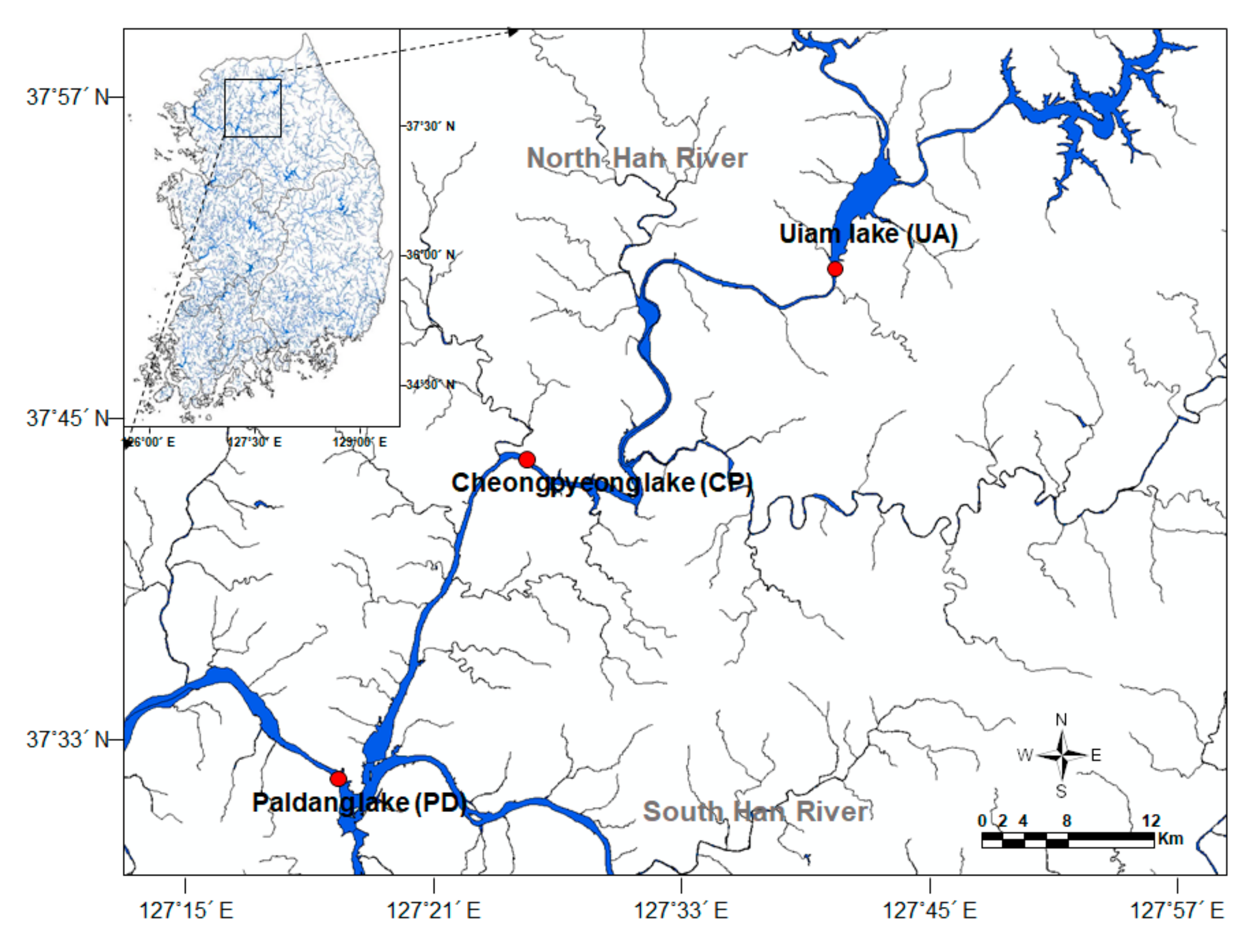
2.1. Ecological Data
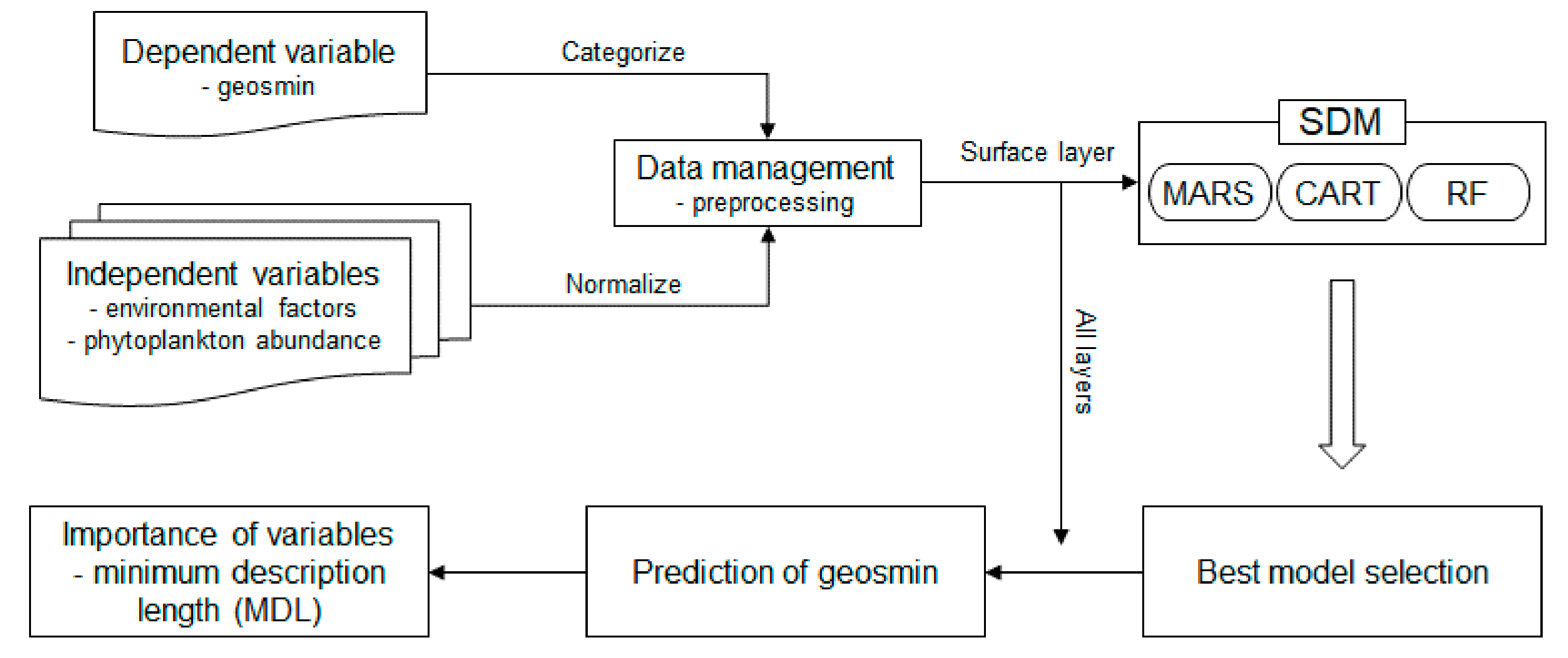
The mean annual temperature and the total amount of annual precipitation in the Han River watershed, which includes Uiam lake, Cheongpyeon lake and Paldang lake during the last 10 years was 10.5 °C and 1319 mm, respectively. Almost 70% of the total annual precipitation occurs from June to September (Korea Meteorological Administration, http://www.kma.go.kr/ (accessed on 17 September 2021)). The morphometric and hydrological characteristics of the three lakes are indicated in Table 1. The data for the phytoplankton community and the environmental variables were obtained from the Basic Environmental Research Program (Investigation of causes of off-flavor material production by harmful algae and management strategy) operated by the Han River Watershed Management Committee (HRWMC) and the Ministry of Environment (MOE), Korea. Samples were surveyed monthly at three major lakes (Uiam, Cheongpyeong, and Paldang lakes) located in the North-Han River watershed area from May 2014 to December 2015 (Figure 1). We conducted samplings 400 m upstream of the dam and samples were collected from three different layers (i.e., surface, middle, and bottom layers). Because of different water depth in the three lakes, the sampling interval among the three layers was different (Uiam lake: 8 m, Cheongpyeong lake: 13 m, and Paldang lake: 10 m). Some data could not be measured due to freezing of lakes (Uiam lake: January to February 2015; Cheongpyeong lake: November 2014 to February 2015, and December 2015; Paldang lake: December 2014 to February 2015) or missing surveys (April 2015).
Phytoplankton and environmental variables were surveyed according to the sampling protocol of HRWMC [12]. Water samples at each layer for the identification of phytoplankton species and measurement of cell densities were taken using a Van Dorn sampler (Halltech Environmental Inc., Guelph, ON, Canada) and stored in Whirl-Pak bags (250 mL), then fixed with Lugol’s solution (2% final concentration). Cell density was measured using a microscope (Axiostar plus; Zeiss, Jena, Germany) with a Sedgwick-Rafter counting chamber at 200–400× magnification. Phytoplankton were identified to the species level [24,25,26].
Water temperature, pH, DO, conductivity, and turbidity were measured in situ using a water quality logger (YSI-6600D, YSI Inc., Yellow Springs, OH, USA). Other variables, such as BOD, SS, TOC, TN, TP, and chlorophyll-a, were analyzed in the laboratory using standard methods [27] (Table 2). Geosmin was determined using Head Space-Solid Phase MicroExtraction (HS-SPME) and gas chromatography/mass spectrometry (GC/MS; 450-GC, 320-MS, Bruker, Billerica, MA, USA) [14]. A Polydimethylsiloxane (PDMS) fiber (47525-U, Supelco, Sigma-Aldrich, St. Louis, MO, USA) was used for the SPME, helium was the carrier gas, and a VF-5MS column 30 m in length and 0.25 mm in diameter was used for separation. Geosmin concentrations <1 ng/L were considered not detectable (ND).

2.2. Data Analysis

Geosmin concentration was categorized into four groups based on the boxplot method (A: <25%, B: 25–50%, C: 50–75%, D: >75%) (Table 3). To predict geosmin concentration categories based on phytoplankton abundance and environmental variables, we applied three representative machine learning techniques such as multivariate adaptive regression splines (MASR), classification and regression trees (CART), and random forest (RF) (Figure 2). These three different models were chosen by considering model complexity and error [28]. All the machine learning techniques were trained and tested based on 10-fold nested cross-validation (training:test = 9:1). [28]. A total of 47 samples from three lakes were used to construct the model.
After the learning process, each model’s performance was tested based on accuracy and area under an ROC curve (AUC) which was widely applied in ecology e.g., [29]. The accuracy computed the correct prediction rate between predicted and observed data [30]. AUC measures a model’s overall performance [30], and ranges from 0 to 1. As a rule of thumb, AUC values above 0.90 indicate excellent, values between 0.80 and 0.90 indicate good, values between 0.70 and 0.80 indicate fair, and 0.60–0.70 and the values below 0.60 indicate fail according to this model [31]. In each prediction model, the relative importance of independent variables for predicting geosmin concentration was evaluated using minimum description length (MDL), which measures the ability of an attribute to compress data [32]. The MDL values were rescaled to range from 0 to 100 to compare the relative importance of each environmental factor. Importance values provided by the algorithm were averaged after 10 repetitions. The prediction models were run in the R computing environment (https://cran.r-project.org/ (accessed on 8 July 2021)) with packages earth [33], rpart [34], and CORElearn [35] for the MARS, CART, and RF models, respectively.
To remove the effect of unit differences [36], all of the independent variables were normalized to the standard deviation of each variable using Formula (1) after natural log (ln (x + 1)) transformation.
(x − avg)/stdev,
where x is a response variable, avg is the average of a response variable, and stdev is the standard deviation of a response variable. Before analyzing the data, all the outlier and extreme values by sampling error were deleted using the boxplot method [37].

3. Results

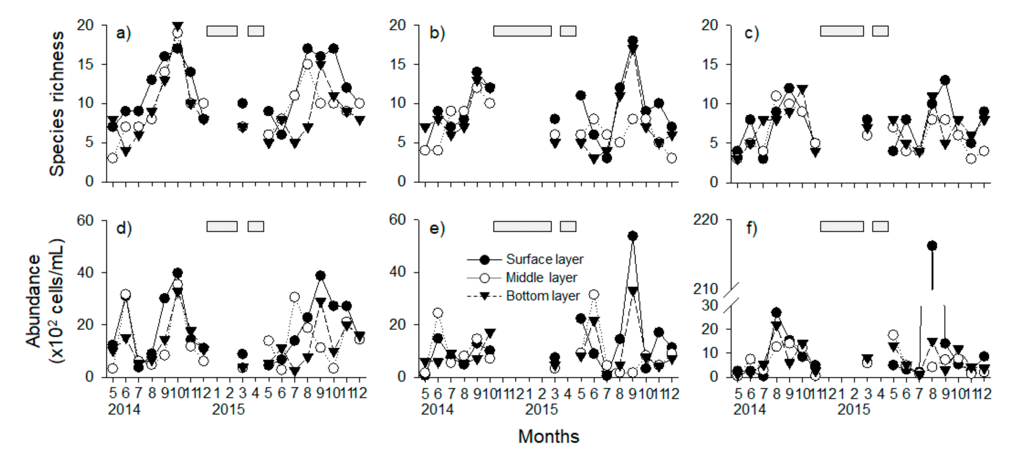
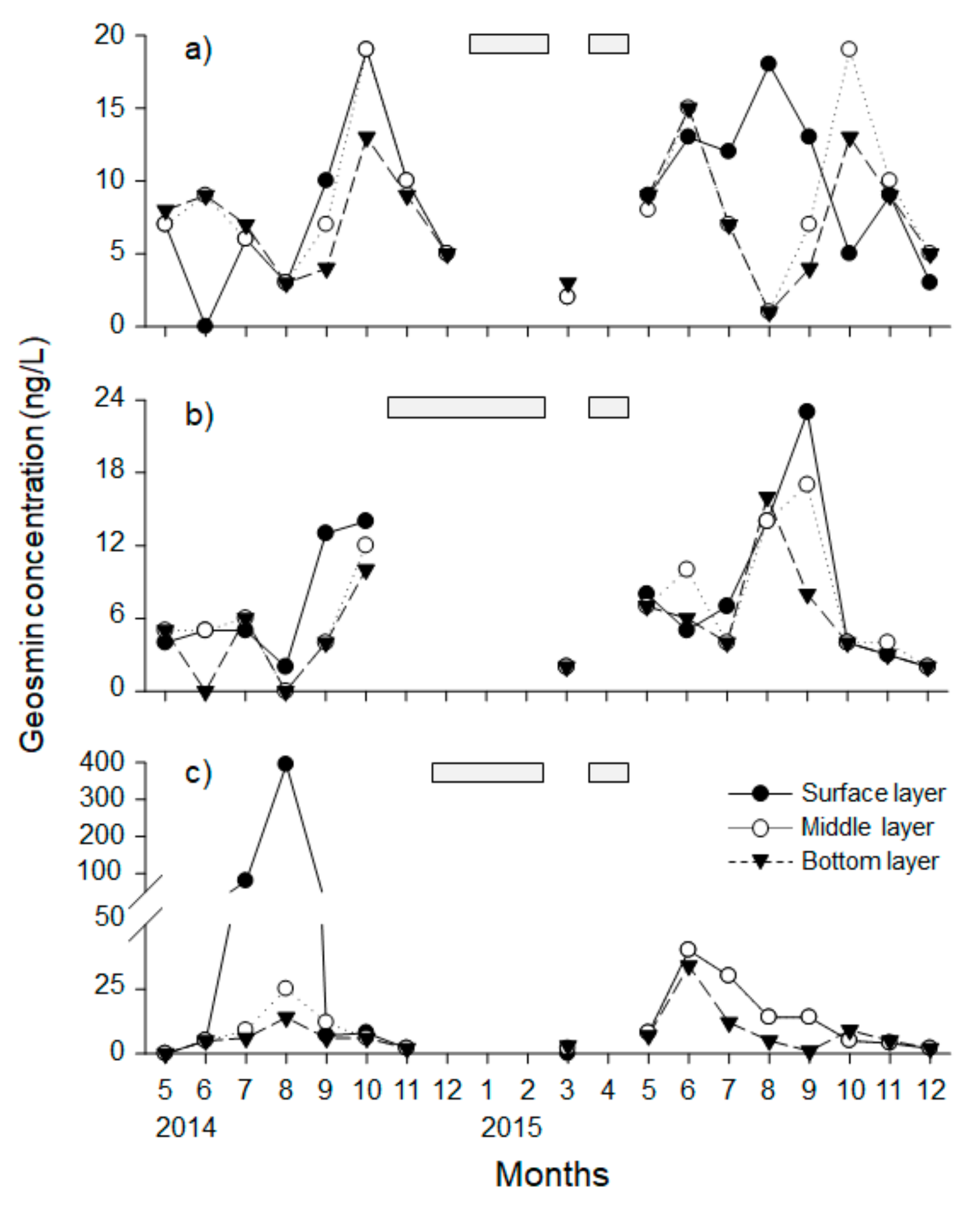
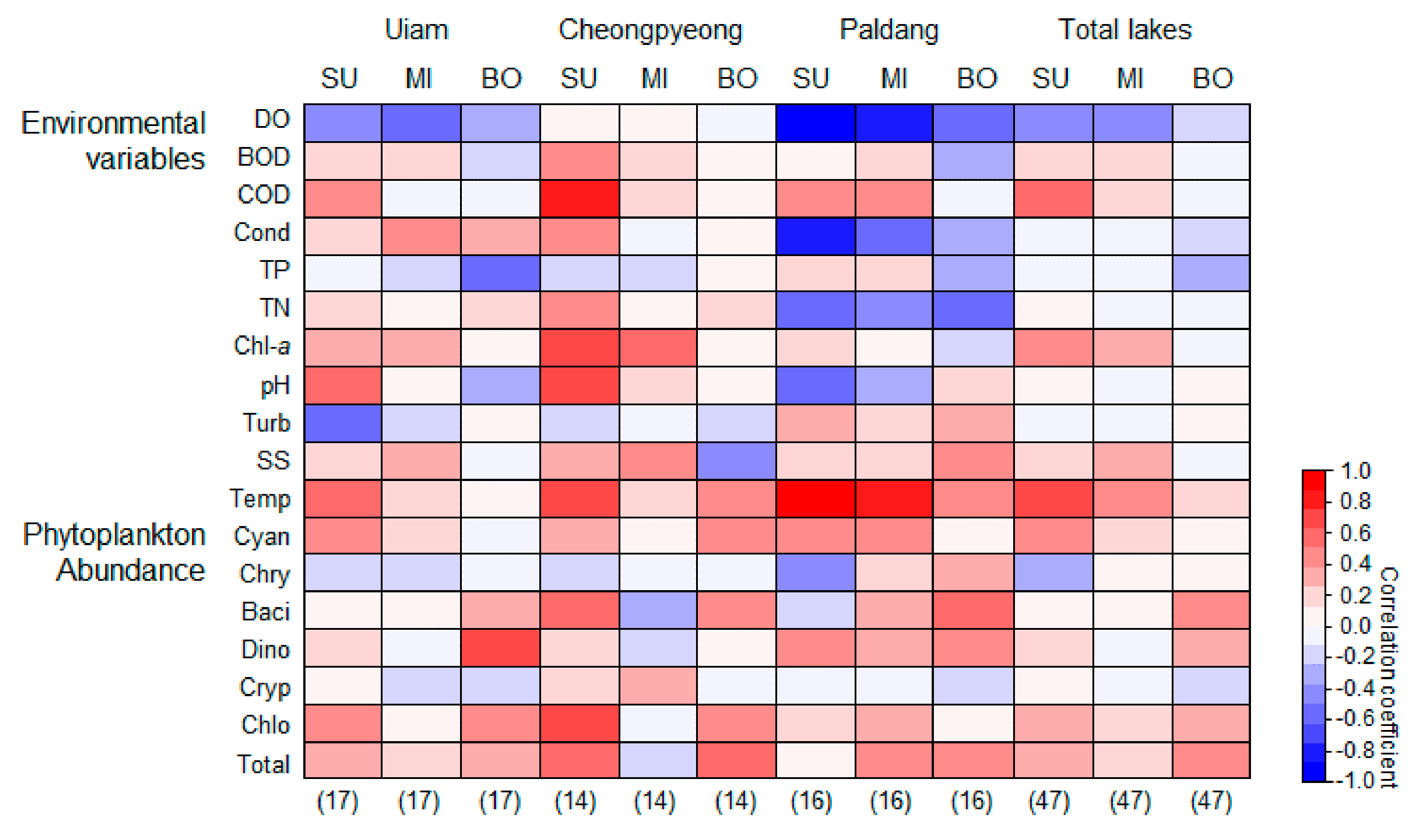
3.1. Relations between Geosmin and Phytoplankton Abundance and Environmental Variables

Species richness and abundance of phytoplankton communities showed clear seasonal dynamics at the three different depths of each lake (except in winter, when data could not be collected due to freezing conditions) (Figure 3). Species richness and abundance of phytoplankton communities were highest at all depths between August and October, and especially in the surface layer during most of the sampling period. Meanwhile, the abundance of phytoplankton communities was the highest in the surface layer of Paldang lake in August 2015 (21,624 cells/mL). The changes of species richness and abundance of phytoplankton communities in Uiam Lake was a significant positive correlation among three layers except for the species richness in the middle and bottom layer (r > 0.50, p < 0.05), whereas Cheongpyeong Lake significantly correlates with species richness only between the surface and bottom layers (r = 0.70, p < 0.05).
Geosmin concentration showed a similar pattern to that of phytoplankton communities, and was higher in summer (June to October) than other periods (Figure 4). In particular, the concentration of geosmin in Paldang Lake exhibited very high values of 394 ng/L and 80 ng/L, respectively, in August and July 2014, but all the rest showed a concentration below 40 ng/L. Meanwhile, the monthly average geosmin concentration was highest in the upper layer (18 ng/L) among three different depths, and the concentration decreased toward the bottom layer (7 ng/L). The changes of geosmin concentrations showed a significant positive correlation among three layers in Cheongpyeong Lake and Paldang Lake (r > 0.64, p < 0.05), and positively correlated between middle and bottom layer in Uiam Lake (r = 0.92, p < 0.05).
We used Spearman’s rank correlation to evaluate the relationship of geosmin concentration with phytoplankton abundance and environmental variables (Figure 5). Geosmin concentration in the surface layer of the total lake (sum of the three lakes) was positively correlated with the abundance of Cyanophyceae (r = 0.44, p < 0.05) and Chlorophyceae (r = 0.32, p < 0.05), while the abundance of Bacillariophyceae (r = 0.39, p < 0.05), Dinophyceae (r = 0.34, p < 0.05), Chlorophyceae (r = 0.30, p < 0.05), and total phytoplankton (r = 0.42, p < 0.05) showed a positive correlation with geosmin concentration in the bottom layers of total lake (sum of the three lakes). Meanwhile, geosmin concentration was negatively correlated with the DO of the surface (r = −0.79, p < 0.05) and middle (r = −0.76, p < 0.05) layers in Paldang, and positively correlated with the water temperature in the surface layer of all lakes (Uiam lake r = 0.54, Cheongpyeong lake r = 0.59, Paldang lake r = 0.82, p < 0.05).

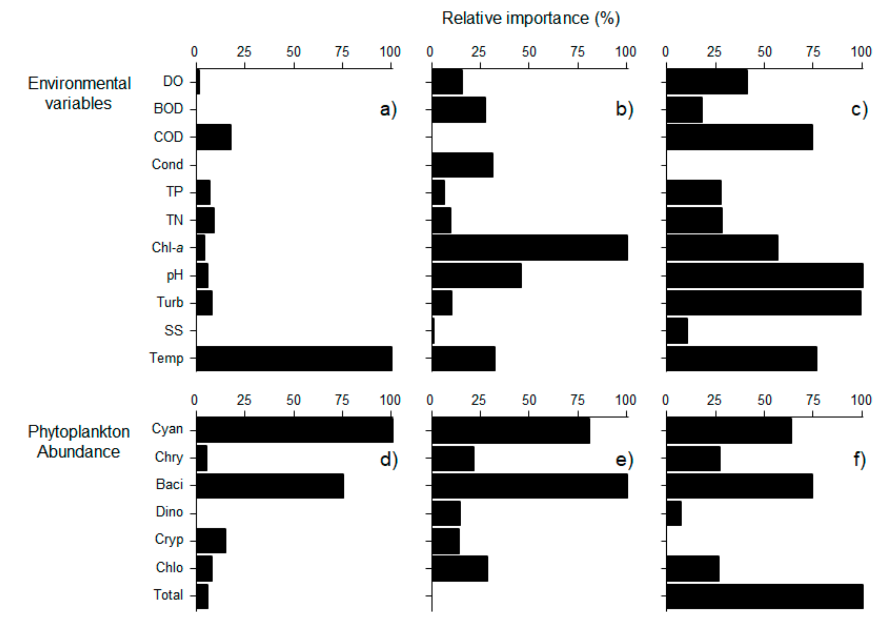
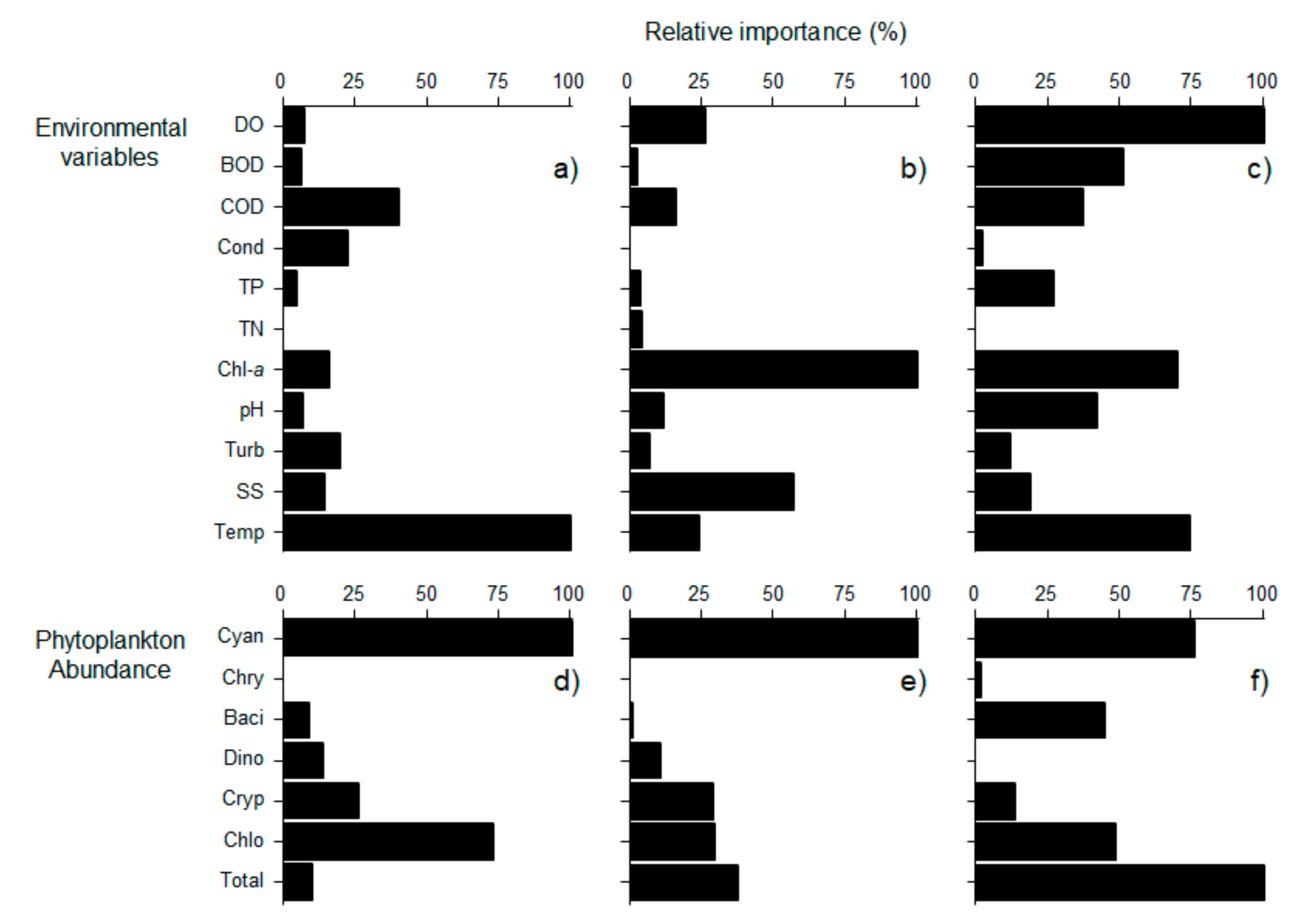
3.2. Prediction of Geosmin Concentration

To predict the geosmin concentration categories, we used three different SDMs—MARS, CART, and RF—according to environmental variables and phytoplankton abundance (Table 4). The RF model performed best in terms of both environmental variables and phytoplankton abundance (AUC > 0.910, accuracy > 0.680); in particular, the prediction of the category with the highest geosmin concentration with environmental variables showed the highest predictive power (AUC: 0.969, accuracy: 0.872). The prediction of the category with the highest geosmin concentration was more predictable in all three SDMs than the prediction of four categories. Meanwhile, MARS exhibited the worst predictive performance in the prediction of four categories (AUC: 0.623, accuracy: 0.447) and the prediction of highest geosmin concentration (AUC: 0.780, accuracy: 0.745) when only phytoplankton abundance data were used.
The RF model, which had the highest predictive power with environmental variables and phytoplankton abundance data among the three SDMs, was applied to the three different water layers (Table 5). All three different layers were well predicted by RF models using environmental variables and phytoplankton abundance (prediction accuracy > 0.610).
The sensitivity analysis was conducted to evaluate the contribution of environmental variables and phytoplankton abundance in predicting the geosmin concentration categories using the MDL values in the RF model (Figure 6 and Figure 7). The relative importance of environmental variables and phytoplankton abundance was different for each layer. The abundance of Cyanophyceae exhibited relatively higher importance in its contribution to the prediction of the four categories in all three layers, particularly so in the surface layer (Figure 6). Among environmental variables, temperature was the most important variable for the prediction of the four categories in the surface layer, whereas chlorophyll and pH were the most influential variables for the prediction of the four categories in the middle and bottom layers, respectively. Meanwhile, abundance of Bacillariophyceae was the most influential variable for the prediction of the four categories in the middle layer, and total abundance showed relatively higher importance in the bottom layer.
In addition, when only the category with highest geosmin concentration was predicted, a similar pattern as that for the prediction of the four categories was observed. Cyanophyceae was the most influential variable in the surface and middle layers (Figure 7). In the bottom layer, total phytoplankton abundance showed relatively high importance. Among environmental variables, temperature was relatively important in the surface and bottom layers, whereas DO was the most influential variable in the bottom layer (Figure 7).

4. Discussion

In the process of proliferation, some algae produce various types of toxin materials and metabolites that cause earthy/moldy taste and odor such as geosmin and MIB [4,8]. Although they are not toxic at concentrations that can occur in water and fish and neither has been associated with serious health effects, they can cause tap water to smell and taste unpleasant [7]. In fact, Ömür-Özbek and Dietrich [38] reported that taste-and-odor problems became an issue after surface waters were used as drinking water sources in many places such as Europe, the Americas, and Japan [39,40]. Taste-and-odor metabolites cannot be removed by conventional water treatment operations such as coagulation and sedimentation. Thus, advanced water treatment processes like granular activated carbon (GAC) or ozone, which incur high financial costs, are used to remove these compounds [5,6,8]. Therefore, taste-and-odor compounds have been the subject of major interest in water management of water supply sources [3]. In this study, we analyzed the change in geosmin concentration at three different depths in the North-Han River watershed and its relationship with environmental variables and phytoplankton abundances using three different SDMs.
Geosmin concentration in the North-Han River watershed from May 2014 to December 2015 was categorized into four groups based on the boxplot method (Table 3), and the concentration of geosmin in group D, which shows the highest concentration, was found to be in the range of 10 ng/L or more. Taste-and-odor compounds such as geosmin can be detected by human noses at 5–10 ng/L, although this varies from individual to individual [41]. Accordingly, the drinking water quality standard in Japan has set the acceptable concentration of geosmin at 10 ng/L or less [42], whereas Korea manages its geosmin concentration below 20 ng/L [14].
Of the SDMs, each modeling approach used in the analysis of ecological data has its strengths and weaknesses, and seemingly only small differences exist in the accuracies of the models [28,43]. In this study, multiple criteria, such as accuracy and AUC, were applied to solve these problems and to select the most suitable model for predicting geosmin concentration categories. Indeed, the predictive performances of the three SDMs were different (Table 4). Among the three SDMs in this study, the RF model showed the highest prediction power for the geosmin categories in terms of both environmental variables and phytoplankton abundance. In particular, the AUC value of the RF model at all layers showed above 0.9 (Table 5), indicating that it was an excellent model according to Swets [31]. Similarly, Harris and Graham [2] reported that the RF model was the best-suited model for the prediction of geosmin concentration under 20 ng/L. As a prediction model, RF is a powerful tool for the analysis of ecological data due several advantages it possesses, such as high classification accuracy, a novel method of determining variable importance, and the ability to model complex interactions among predictor variables [44,45].
Cyanobacteria blooms mainly cause abnormal growth of phytoplankton, but can seriously affect drinking water supply due to cyanobacteria metabolites such as toxins and taste substances [2]. In our results, geosmin concentrations were shown to be high during the summer, when phytoplankton abundance increased due to cyanobacteria blooms (Figure 4 and Figure 5). Generally, Anabaena spp., major blue-green algae, are the most representative species producing geosmin worldwide [46]. In particular, cyanobacteria such as Anabaena, Aphanizomenon, Oscillatoria, and Microcystis are the main group of microorganisms that are responsible for the earthy-musty odor in drinking water, and are mostly found as surface scum and benthic mat in eutrophic waters [47,48,49,50]. In particular, according to previous studies [51,52], A. circinalis had proliferated and had been observed in the form of scum in the surface layer of Paldang Lake after July 2014; consequently, the concentration of geosmin had rapidly increased. After August 2014, however, the geosmin concentration had sharply decreased due to the dilution effect caused by the confluence of upstream and seasonal rain, combined with the flushing effect caused by the opening of the dam [53,54].
Meanwhile, temporal changes in both the phytoplankton community and geosmin concentration according to depth were different for each lake (Figure 3 and Figure 4). The change in geosmin concentration has been shown to be positively related to the amount of A. spiroides [55]. This was reflected in our study, in that the relative importance of Cyanophyceae abundance was highest in the RF model for predicting the categories of geosmin concentration (Figure 6 and Figure 7). The relative importance of temperature was also the highest among the environmental factors in the surface layer of the lake in this study (Figure 6 and Figure 7), because the decrease of water temperature had the greatest effect on the reduction of A. spiroides. The dominant period of Cyanophyceae can be determined by the trophic state and water temperature of the lakes, and low water temperature in winter is a major contributor to the extinction of Cyanophyceae [56,57,58]. Furthermore, turbidity, which was relatively high in terms of importance in the bottom layer, exhibited such high importance due to its relationship with the light environment for algae growth [4]. These depth-variable environmental variables are likely to be the key factors driving changes in the composition of the phytoplankton community [59].

5. Conclusions

In this study, the RF method demonstrated the best predictive power for geosmin concentration categories in the surface layer of lakes among the three machine-learning techniques (MARS, CART, and RF). Therefore, in the RF model approach for the further analysis (i.e., estimating the geosmin concentration categories with environmental variables and phytoplankton abundance at different lake depths), the model showed higher prediction in case of only predicting the highest geosmin concentration category compared with predicting four categories based on the boxplot. The sensitivity analysis of the model showed that temperature and Cyanophyceae abundance were highly important in the prediction of geosmin concentration categories in the surface layer, whereas total phytoplankton abundance was important for predicting geosmin concentration categories in the bottom layer.

Author Contributions

Conceptualization, Y.-S.K., M.-J.B. and B.-H.K.; methodology, Y.-S.K. and I.-H.C.; formal analysis, Y.-S.K. and I.-H.C.; investigation, I.-H.C., H.-K.K. and J.-H.B.; data curation, I.-H.C. and J.-H.B.; writing—original draft preparation, Y.-S.K., I.-H.C., M.-J.B. and B.-H.K.; writing—review and editing, Y.-S.K., I.-H.C., H.-K.K., J.-H.B. and B.-H.K.; supervision, B.-H.K. All authors have read and agreed to the published version of the manuscript.

Funding

This work was supported by a grant from the National Institute of Ecology (NIE-B-2021-01), and National Institute of Environmental Research (NIER-2021-01-01-085), funded by the Ministry of Environment (MOE) of the Republic of Korea.

Institutional Review Board Statement

Not applicable.

Informed Consent Statement

Not applicable.

Conflicts of Interest

The authors declare no conflict of interest.

References

  1. Bruder, S.; Babbar-Sebens, M.; Tedesco, L.; Soyeux, E. Use of fuzzy logic models for prediction of taste and odor compounds in algal bloom-affected inland water bodies. Environ. Monit. Assess. 2014, 186, 1525–1545. [Google Scholar] [CrossRef]
  2. Harris, T.D.; Graham, J.L. Predicting cyanobacterial abundance, microcystin, and geosmin in a eutrophic drinking-water reservoir using a 14-year dataset. Lake Reserv. Manag. 2017, 33, 32–48. [Google Scholar] [CrossRef]
  3. Dodds, W.K.; Bouska, W.W.; Eitzmann, J.L.; Pilger, T.J.; Pitts, K.L.; Riley, A.J.; Schloesser, J.T.; Thornbrugh, D.J. Eutrophication of U.S. freshwaters: Analysis of potential economic damages. Environ. Sci. Technol. 2009, 43, 12–19. [Google Scholar] [CrossRef] [Green Version]
  4. Christensen, V.G.; Graham, J.L.; Milligan, C.R.; Pope, L.M.; Zeigler, A.C. Water quality and relation to tasteand-odor compounds in the North Fork Ninnescah River and Cheney Reservoir, Southcentral Kansas, 1997–2003. In Scientific Investigations Report 2006–5095; US Geological Survey: Reston, VA, USA, 2006; pp. 1–43. [Google Scholar] [CrossRef]
  5. Chung, S.-W.; Chong, S.A.; Park, H.-S. Development and applications of a predictive model for geosmin in North Han River, Korea. Procedia Eng. 2016, 154, 521–528. [Google Scholar] [CrossRef]
  6. Srinivasan, R.; Sorial, G.A. Treatment of taste and odor causing compounds 2-mdethyl isoborneol and geosmin in drinking water: A critical review. J. Environ. Sci. 2011, 23, 1–13. [Google Scholar] [CrossRef]
  7. Smith, V.H.; Sieber-Denliger, J.; DeNoyelles, F.; Campbell, S.; Pan, S.; Randtke, S.J.; Blain, G.T.; Strasser, V.A. Managing taste and odor problems in a eutrophic drinking water reservoir. Lake Reserv. Manag. 2002, 18, 319–323. [Google Scholar] [CrossRef] [Green Version]
  8. Watson, S.B. Aquatic taste and odour: A primary signal of drinking water integrity. J. Toxicol. Environ. Health 2004, 67, 1779–1795. [Google Scholar] [CrossRef] [PubMed]
  9. Gerber, N.N.; Lechevalier, H.A. Geosmin, and earthy-smelling substances isolated from actinomycetes. Appl. Microbiol. 1967, 13, 935–938. [Google Scholar] [CrossRef] [PubMed]
  10. Safferman, R.S.; Rosen, A.A.; Mashni, C.I.; Morris, M.E. Earthy-smelling substance from a blue-green alga. Environ. Sci. Technol. 1967, 1, 429–430. [Google Scholar] [CrossRef] [PubMed]
  11. Hsieh, W.-H.; Chang, D.-W.; Lin, T.-F. Occurrence and removal of earthy-musty odorants in two waterworks in Kinmen Island, Taiwan. J. Hazard. Toxic Radioact. Waste 2014, 18, 04014012. [Google Scholar] [CrossRef]
  12. Watershed, H.R. Watershed and Environment Management District (HRWEMD). In Distribution and Eco-Physiological Characteristics of Harmful Algae in the North Han River. Final Report; Han River Watershed Management Commission: Hanam, Korea, 2013. (In Korean) [Google Scholar]
  13. You, K.-A.; Byeon, M.-S.; Youn, S.-J.; Hwang, S.-J.; Rhew, D.-H. Growth characteristics of blue-green algae (Anabaena spiroides) causing tastes and odors in the North-Han River, Korea. Korean J. Ecol. Environ. 2013, 46, 135–144. [Google Scholar] [CrossRef]
  14. Ministry of Environment (MOE). Drinking Water Quality Monitoring Guideline; Ministry of Environment: Sejong-si, Korea, 2014. (In Korean)
  15. Ma, Z.; Xie, P.; Chen, J.; Niu, Y.; Tao, M.; Qi, M.; Zhang, W.; Deng, X. Microcystis blooms influencing volatile organic compounds concentrations in Lake Taihu. Fresenius Environ. Bull. 2013, 22, 95–102. [Google Scholar]
  16. Yagi, M.; Kajino, M.; Matsuo, U.; Ashitani, K.; Kita, T.; Nakamura, T. Odor problems in Lake Biwa. Water Sci. Technol. 1983, 15, 311–321. [Google Scholar] [CrossRef]
  17. Romero, J.; Ventura, F. Occurrence of Geosmin and Other Odorous Compounds of Natural Origin in Surface and Drinking Waters. A Case Study. Intern. J. Environ. Anal. Chem. 2000, 77, 243–254. [Google Scholar] [CrossRef]
  18. Jones, G.J.; Korth, W. In situ production of volatile odor compounds by river and reservoir phytoplankton populations in Australia. Water Sci. Technol. 1995, 31, 145–151. [Google Scholar] [CrossRef]
  19. Wnorowski, A.U.; Scott, W.E. Incidence of off-flavors in South-African surface waters. Water Sci. Technol. 1992, 1992. 25, 225–232. [Google Scholar] [CrossRef]
  20. Parinet, J.; Rodriguez, M.J.; Sérodes, J.-B. Modelling geosmin concentrations in three sources of raw water in Quebec, Canada. Environ. Monit. Assess. 2013, 185, 95–111. [Google Scholar] [CrossRef]
  21. Sugiura, N.; Utsumi, M.; Wei, B.; Iwami, N.; Okana, K.; Kawauchi, Y.; Maekawa, T. Assessment for the complicated occurrence of nuisance odours from phytoplankton and environmental factors in a eutrophic lake. Lakes Reserv. Res. Manag. 2004, 9, 195–201. [Google Scholar] [CrossRef]
  22. Dzialowski, A.R.; Smith, V.H.; Huggins, D.G.; deNoyelles, F.; Lim, N.C.; Baker, D.S.; Beury, J.H. Development of predictive models for geosmin-related taste and odor in Kansas, USA, drinking water reservoirs. Water Res. 2009, 43, 2829–2840. [Google Scholar] [CrossRef]
  23. Chong, S.; Lee, H.; An, K.-G. Predicting taste and odor compounds in a shallow reservoir using a three–dimensional hydrodynamic ecological model. Water 2018, 10, 1396. [Google Scholar] [CrossRef] [Green Version]
  24. Cox, E.J. Identification of Freshwater Diatoms from Live Material; Chapman & Hall: London, UK, 1996. [Google Scholar]
  25. Akiyama, M.; Loiya, T.; Imahori, K.; Kasaki, H.; Kumano, S.; Kobayashi, H.; Takahashi, E.; Tsumura, K.; Hirano, M.; Hirose, H.; et al. Illustration of the Japanese Freshwater Algae; Uchida Rockakuho Publishing Co.: Tokyo, Japan, 1977. [Google Scholar]
  26. Abe, T.H. Studies on the Order Peridinidae an Unfinished Monograph of the Armoured Dinoflagellata; The Nippon Printing and Publishing Co.: Tokyo, Japan, 1981. [Google Scholar]
  27. American Public Health Association (APHA). Standard Methods for the Examination of Water and Wastewater, 21st ed.; American Public Health Association: Washington, DC, USA, 2005. [Google Scholar]
  28. Fukuda, S.; de Baets, B.; Waegeman, W.; Verwaeren, J. Habitat prediction and knowledge extraction for spawning European grayling (Thymallus thymallus L.) using a broad range of species distribution models. Environ. Model. Softw. 2013, 47, 1–6. [Google Scholar] [CrossRef]
  29. Garzón, M.B.; Blazek, R.; Neteler, M.; de Dios, R.S.; Ollero, H.S.; Furlanello, C. Predicting habitat suitability with machine learning models: The potential area of Pinus sylvestris L. in the Iberian Peninsula. Ecol. Model. 2006, 197, 383–393. [Google Scholar] [CrossRef]
  30. Buisson, L.; Grenouillet, G.; Casajus, N.; Lek, S. Predicting the potential impacts of climate change on stream fish assemblages. Am. Fish. Soc. Symp. 2010, 73, 327–346. [Google Scholar] [CrossRef]
  31. Swets, J.A. Measuring the accuracy of diagnostic systems. Science 1988, 240, 1285–1293. [Google Scholar] [CrossRef] [PubMed] [Green Version]
  32. Robnik-Šikonja, M. Improving Random Forests. In Machine Learning ECML 2004; Boulicaut, J.-F., Esposito, F., Giannotti, F., Pedreschi, D., Eds.; Springer: Berlin/Heidelberg, Germany, 2004; pp. 359–370. [Google Scholar] [CrossRef] [Green Version]
  33. Milborrow, S. Earth: Multivariate Adaptive Regression Splines. R Package. Version 5.3.0. Available online: https://cran.r-project.org/ (accessed on 8 July 2021).
  34. Therneau, T.; Atkinson, B.; Ripley, B. Rpart: Recursive Partitioning and Regression Trees. R package. Version 4.1-15. Available online: https://cran.r-project.org/bin/windows/ (accessed on 8 July 2021).
  35. Robnik-Sikonja, M.; Savicky, P. CORElearn: CORElearn—Classification, Regression, Feature Evaluation. R Package. Version 1.54.2. Available online: https://cran.r-project.org/bin/windows/base/ (accessed on 8 July 2021).
  36. Peterson, A.T.; Soberón, J.; Pearson, R.G.; Anderson, R.P.; Martinez-Meyer, E.; Nakamura, M.; Araújo, M.B. Ecological Niches and Geographical Distributions; Princeton University Press: Princeton, NJ, USA, 2011. [Google Scholar]
  37. Helsel, D.R.; Hirsch, R.M. Statistical Methods in Water Resources; Elsevier: Amsterdam, The Netherlands, 1992. [Google Scholar]
  38. Ömür-Özbek, P.; Dietrich, A.M. Determination of Temperature-Dependent Henry’s Law Constants of Odorous Contaminants and Their Application to Human Perception. Environ. Sci. Technol. 2005, 2005. 39, 3957–3963. [Google Scholar] [CrossRef]
  39. Magara, Y.; Kunikane, S. Cost analysis of the adverse effects of algal growth in water bodies on drinking water supply. Ecol. Model. 1986, 1986. 31, 303–313. [Google Scholar] [CrossRef]
  40. Yagi, M. Musty odour problems in lake Biwa, 1982–1987. Water Sci. Technol. 1988, 1988. 20, 133–142. [Google Scholar] [CrossRef]
  41. Cook, D.; Newcombe, G.; Sztajnbok, P. The application of powdered activated carbon for MIB and geosmin removal: Predicting PAC doses in four raw waters. Water Res. 2001, 35, 1325–1333. [Google Scholar] [CrossRef]
  42. Whelton, A.J.; Dietrich, A.M. Relationship between intensity, concentration, and temperature for drinking water odorants, Water Res. 2004. Water Res. 2004, 38, 1604–1614. [Google Scholar] [CrossRef]
  43. Segurado, P.; Araújo, M. An evaluation of methods for modelling species distributions. J. Biogeogr. 2004, 2004. 31, 1555–1568. [Google Scholar] [CrossRef]
  44. Cutler, D.R.; Edwards, T.C., Jr.; Beard, K.H.; Cutler, A.; Hess, K.T.; Gibson, J.; Lawler, J.J. Random forests for classification in ecology. Ecology 2007, 88, 2783–2792. [Google Scholar] [CrossRef]
  45. Kwon, Y.-S.; Bae, M.-J.; Hwang, S.-J.; Kim, S.-H.; Park, Y.-S. Predicting potential impacts of climate change on freshwater fish in Korea. Ecol. Inform. 2015, 29, 156–165. [Google Scholar] [CrossRef]
  46. Tsao, H.W.; Michinaka, A.; Yen, H.K.; Giglio, S.; Hobson, P.; Monis, P.; Lin, T.F. Monitoring of geosmin producing Anabaena circinalis using quantitative PCR. Water Res. 2014, 49, 416–425. [Google Scholar] [CrossRef] [PubMed]
  47. Smith, J.L.; Boyer, G.L.; Zimba, P.V. A review of cyanobacterial odorous and bioactive metabolites: Impacts and management alternatives in aquaculture. Aquaculture 2008, 280, 5–20. [Google Scholar] [CrossRef]
  48. Jüttner, F.; Watson, S.B. Biochemical and ecological control of geosmin and 2-methylisoborneol in source waters. Appl. Environ. Microbiol. 2007, 73, 4395–4406. [Google Scholar] [CrossRef] [PubMed] [Green Version]
  49. Watson, S.B.; Monis, P.; Baker, P.; Giglio, S. Biochemistry and genetics of taste- and odor-producing cyanobacteria. Harmful Algae 2016, 54, 112–127. [Google Scholar] [CrossRef] [PubMed]
  50. Watson, S.B. Cyanobacterial and eukaryotic algal odour compounds: Signal or by-product? A review of their biological activity. Phycologia 2003, 42, 332–350. [Google Scholar] [CrossRef]
  51. Byun, J.H.; Hwang, S.J.; Kim, B.H.; Park, J.R.; Lee, J.K.; Lim, B.J. Relationship between a dense population of cyanobacteria and odorous compounds in the North Han River system in 2014 and 2015. Korean J. Ecol. Environ. 2015, 48, 263–271. [Google Scholar] [CrossRef]
  52. Youn, S.J.; Kim, Y.-J.; Kim, H.-N.; Kim, J.-Y.; Yu, M.-N.; Lee, E.J.; Yu, S.J. Geosmin and morphological characteristics of Anabaena circinalis, obtained from the Bukhan River. J. Environ. Sci. Int. 2018, 2018. 27, 27–38. [Google Scholar] [CrossRef]
  53. Ward, J.V.; Stanford, J.A. The serial discontinuity concept of lotic ecosystems. In Dynamics of Lotic Ecosystems; Fontaine, T.D., Bartell, S.M., Eds.; Ann Arbor Science: Ann Arbor, MI, USA, 1983; pp. 29–42. [Google Scholar]
  54. Byun, J.H.; Cho, I.H.; Hwang, S.J.; Park, M.H.; Byeon, M.S.; Kim, B.H. Relationship between a dense bloom of cyanobacterium Anabaena spp. and rainfalls in the North Han River system of South Korea. Korean J. Ecol. Environ. 2014, 2014. 47, 116–126. [Google Scholar] [CrossRef]
  55. Li, Z.; Yu, J.; Yang, M.; Zhang, D.; Burch, M.D.; Han, W. Cyanobacterial population and harmful metabolites dynamics during a bloom in Yanghe Reservoir, North China. Harmful Algae 2010, 9, 481–488. [Google Scholar] [CrossRef]
  56. Reynolds, C.S. Phytoplankton periodicity the interactions of form, function and environmental variability. Freshw. Biol. 1984, 14, 11–42. [Google Scholar] [CrossRef]
  57. Sommer, U.; Gliwicz, Z.M.; Lampert, W.; Duncan, A. The PEG-model of seasonal succession of planktonic events in fresh waters. Arch. Für Hydrobiol. 1986, 106, 433–471. [Google Scholar]
  58. Romo, S.; Miracle, M.R. Population dynamics and ecology of subdominant phytoplankton species in a shallow hypertrophic lake (Albufera of Valencia, Spain). Hydrobiologia 1994, 273, 37–56. [Google Scholar] [CrossRef]
  59. Kwon, Y.; Hwang, S.; Park, K.; Kim, H.; Kim, B.; Shin, K.; An, K.; Song, Y.; Park, Y. Temporal changes of phytoplankton community at different depths of a shallow hypertrophic reservoir in relation to environmental variables. Ann. Limnol. Int. J. Limnol. 2009, 45, 93–105. [Google Scholar] [CrossRef] [Green Version]
Figure 1. Locations of the study sites () in the Han River watershed of South Korea.
Ijerph 18 10303 g001
Figure 2. Flow chart of the modeling procedures to predict geosmin concentration categories based on phytoplankton abundance and environmental variables.
Ijerph 18 10303 g002
Figure 3. Temporal dynamics of the species richness and abundance of phytoplankton communities in three lakes—Uiam (a,d), Cheongpyeong (b,e), and Paldang (c,f)—from May 2014 to December 2015. Gray bars indicate data loss/missing data due to freezing conditions or missing survey.
Ijerph 18 10303 g003
Figure 4. Temporal variation of geosmin at three different water depths in three lakes—(a) Uiam, (b) Cheongpyeong, (c) Paldang lake—from May 2014 to December 2015. Gray bar indicates data loss/missing due to freezing conditions or missing survey.
Ijerph 18 10303 g004
Figure 5. Correlation between geosmin and phytoplankton abundance and environmental variables. The color gradient (from −1 to 1) indicates Spearman’s correlation coefficients. The darker red indicates a higher positive correlation (p < 0.05), and darker blue indicates a higher negative correlation (p < 0.05). The numbers in parenthesis indicate the number of sampling sizes. Abbreviation of each variable indicated in Table 2. SU: surface layer, MI: middle layer, BO: bottom layer, and Total lake: pooled sample in each layer from three lakes.
Ijerph 18 10303 g005
Figure 6. Relative importance (%) of environmental variables (ac) and phytoplankton abundance (df) in predicting the four categories (A–D) of geosmin concentration in three different depths. Surface layer (a,d), Middle layer (b,e), and Bottom layer (c,f). Abbreviation of each variable indicated in Table 2.
Ijerph 18 10303 g006
Figure 7. Relative importance (%) of environmental variables (ac) and phytoplankton abundance (df) in predicting category with highest geosmin concentration (D) in three different depths. Surface layer (a,d), Middle layer (b,e), and, Bottom layer (c,f). Abbreviation of each variable indicated in Table 2.
Ijerph 18 10303 g007
Table 1. Information of morphometric and hydrological characteristics in three lakes in the study.
FactorsLakes
UiamCheongpyeongPaldang
Watershed area (km2)7709992123,800
Total storage (106 m3)80185.5244
Effective storage (106 m3)57.5282.618
Inflow (106 m3/year)5323683717,020
Outflow (106 m3/year)5322683616,988
Dam height (m)233129
Residence time (day)7.39.312.9
Table 2. Summary of 19 variables used in the prediction model (units, methods of measurement and abbreviations).
VariablesAbbreviationUnitsMethods
Independent variablesCyanophyceaeCyancell/mL-
ChrysophyceaeChrycell/mL-
BacillariophyceaeBacicell/mL-
DinophyceaeDinocell/mL-
CryptophyceaeCrypcell/mL-
ClorophyceaeChlocell/mL-
Total abundanceTotalcell/mL-
Water TemperatureTemp°CMultimeter in the field
ConductivityCondμS/cm
TurbidityTurbNTU
pHpH-
Dissolved OxygenDOmgO2/L
Chemical Oxygen DemandCODmgO2/LCODMn
Biochemical Oxygen DemandBODmgO2/LMembrane Electrode Method
Total PhosphorousTPmg/LAscorbic acid analysis
Total NitrogenTNmg/LAscorptiometric analysis
Suspended SolidSSmg/LGF/C
Chlorophyll aChl-aμg/LAscorptiometric analysis
Dependent variablesGeosmin-ng/LHS-SPME
Table 3. Categories of geosmin concentration were defined based on the boxplot method. The numbers in parenthesis (n) indicate the number of sampling sizes.
CategoryA (≤25%)B (25–50%)C (50–75%)D (>75%)
Range of geosmin (n)≤4 (45)4–6 (28)6–10 (34)>10 (34)
Table 4. Comparison of the predictive performance of three different models with different combinations of independent variables (environmental variables and phytoplankton abundance). CART: classification and regression tree, MARS: multivariate adaptive regression splines, and RF: random forest. Categories (A–D) of geosmin concentration are given in Table 3.
DatasetModelEnvironmental VariablesPhytoplankton Abundance
AUCAccuracyAUCAccuracy
Four categories (A–D)MARS0.7240.5530.6230.447
CART0.7610.6170.7130.574
RF0.9740.8090.9340.681
Category with highest geosmin concentration (D)MARS0.9040.8090.7800.745
CART0.7900.8300.8160.787
RF0.9690.8720.9140.851
Table 5. Prediction accuracy of geosmin concentration in three different water layers using random forest model. Categories (A–D) of geosmin concentration are given in Table 3.
DatasetLayerEnvironmental VariablesPhytoplankton Abundance
AUCAccuracyAUCAccuracy
Four categories (A–D)Surface0.9740.8090.9340.681
Middle0.9760.7660.9230.745
Bottom0.9810.7870.9370.617
Category with highest geosmin concentration (D)Surface0.9690.8720.9140.851
Middle0.9670.8510.9060.787
Bottom0.9810.8300.9200.830
Publisher’s Note: MDPI stays neutral with regard to jurisdictional claims in published maps and institutional affiliations.

