Abstract
The current manuscript proposes a control chart for monitoring road accidents and injuries using repetitive sampling. The proposed chart helps in identifying the shifts in accidents and injuries more quickly than existing charts. The application of the proposed chart will help in reducing and identifying the reasons for road accidents and road injuries efficiently.
1. Introduction
Control charts are designed to indicate a shift in the process and help industrialists, services companies, and the policy-makers department brings back the process to its normal state. Control charts have the ability to give prior information on when, on average, the process is going to be out-of-control. Therefore, control charts are wonderful tools to minimize the non-conforming items and increase the profit of industry and service companies. Control charts guide policy-makers in identifying the source of variations that cause the shift in the process from the center. References [1,2] discussed the applications of control charts.
Control charts have been broadly applied in monitoring road accidents, road injuries, and road crashes. Control charts lead highway experts in designing roads to minimize road accidents and injuries. In addition, these are helpful in identifying the factors that cause an increase in road accidents and injuries. The proper monitoring of roads with the help of control charts may significantly reduce road accidents and crashes. The application of control charts in monitoring children’s road injuries was discussed by [3]. The various aspects of road accidents with the help of a control chart were discussed by [4]. References [5,6,7,8] presented the applications of control charts in monitoring road accidents. [1] introduced an exponentially weighted moving average (EWMA) for monitoring road accidents. A good statistical analysis of road accident data was discussed by [9,10]. Reference [11] presented the control charts for monitoring hazardous road accidents. Reference [12] presented the control charts using the Saudi traffic accidents data. [13,14] presented the statistical analysis by using motorcyclist injuries data and road accident data. References [15,16] presented excellent work in monitoring road accidents.
The neutrosophic logic, which is an extension of the fuzzy logic, is applied when indeterminacy is presented in the data [17]. According to [18], neutrosophic logic is more efficient than fuzzy logic and interval-based analysis. Reference [17] argued that neutrosophic statistics are more efficient than classical statistics in terms of the measurement of indeterminacy. Reference [19] proposed the neutrosophic EWMA (NEWMA) control chart for monitoring road accidents. Some other applications of neutrosophic statistics can be seen in [20,21,22]. Reference [23] worked on fuzzy-based non-parametric tests. Reference [24] proposed the median test using fuzzy logic. Reference [25] proposed the life-test using the fuzzy approach. Reference [26] proposed the idea of correlation using the fuzzy sets theory. Reference [27] proposed the signed-rank test for the interval data, and [28] presented the correlation analysis using the Pythagorean fuzzy approach. Reference [29] contributed excellent work in making control charts using functional data. Reference [30] studied the effects of indeterminacy on the performance of control charts.
Shewhart variance control charts are applied to monitor the variation in data. The EWMA variance control charts enhance the power of the Shewhart variance control charts, see [31]. References [32,19] introduced control charts under neutrosophic statistics. Reference [33] proposed a chart using a single sampling scheme. Repetitive sampling is the extension of single sampling and is applied when no decision is made on the basis of single sample information. In repetitive sampling, the process of selecting a sample is repeated when no decision is made on the first sample see [34]. To the best of our knowledge, there is still a gap in the design of variance NEWMA charts, being the control chart using repetitive sampling under neutrosophic statistics. In this paper, a control chart using repetitive sampling under neutrosophic statistics will be introduced and applied in monitoring road accidents and road injuries. It is expected that the proposed chart will be more efficient than the existing charts and better help indicate the shift in road accidents and road injuries compared to the existing charts.
2. The Proposed Chart
Let 1, 2, 3,…, be a neutrosophic random sample from the neutrosophic normal distribution with a neutrosophic mean of and a neutrosophic variance of , where is a neutrosophic sample size. Suppose that denotes the neutrosophic sample mean and presents the neutrosophic sample variance. Reference [33] proposed the following NEWMA statistic as a generalization of the EWMA statistic proposed by [35,36].
Note here that and are a neutrosophic smoothing constant, selected on the basis of personal experience, [37]. Industrial engineers are always uncertain on the selection of a suitable value for . Let denote the indeterminacy or uncertainty parameter. The neutrosophic form of can be expressed as follows
Note here that denotes the values under classical statistics and is also known as the determined part of the neutrosophic form and denotes the indeterminate part of the neutrosophic form. Note here that the neutrosophic form reduces to a smoothing constant under classical statistics when no uncertainty is found in the selection of the smoothing constant.
The values of in Equation (1) can be obtained as follows
Reference [38] showed that is closer to a neutrosophic normal distribution than . Reference [39] state: “the main expectation of this approach is that if , and are judiciously selected, then this transformation may result in approximate normality to ”. The neutrosophic control limits (NCLs) under repetitive sampling with starting values of = 0 are given by:
Note that and present a neutrosophic control limit coefficient associated with NCLs.
The NCLs given in Equations (1)–(4) are approximate but widely applied due to simplicity, see [39]. The exact NCLs for under repetitive sampling are given as:
By following [39], the approximate control limits are considered in this paper.
3. The Proposed Control Chart
As mentioned in [39], the transformation makes the limits that are not symmetrical in a traditional control chart symmetrical. The proposed will be operated as follows:
Step-1: Compute statistic for sample size when indeterminacy parameter is specified.
Step-2: If or , the process is said to be out-of-control. The process is said to be in-control if , otherwise repeat step 1.
The proposed control chart has four control limits. The proposed control chart reduces to the control chart proposed by [33] when no repetition is needed. The probability of being in-control for the proposed control chart is:
where is the probability of repetition and is the probability of being in-control for the single sampling, given by:
The probability of being in-control for the shifted process is given by
where is the probability of repetition and is the probability of in-control for the single sampling, given by:
The neutrosophic average run length (NARL) for the in-control and shifted process are given by
The following is the neutrosophic Monte Carlo (NMS) used to find the values of , and , when is fixed.
- Fix the sample size and generate 10,000 random samples of size and select the values of , and from [33]. Compute the values of the statistic for the specified indeterminacy parameter and plot these values of NCLs.
- Note the first out-of-control values for the 10,000 random samples and compute and neutrosophic standard division (NSD) and select the values of and for which is very close to the specified values of .
- Using the selected values of and , compute for the data generated at various values of shift . Compute the values of and NSD for various values of .
Using the above algorithm, the values of and NSD for various values of , , and are placed in Table 1, Table 2, Table 3, Table 4, Table 5, Table 6. Table 1 is presented for [3,5] and . Table 2 is given for [3,5] and . Table 3 is given for [3,5] and . Table 4 is presented for [8,10] and . Table 5 is given for [8,10] and . Finally, Table 6 is given for [8,10] and . The R codes to make the Tables are given in Appendix A.

Table 1.
The NARL when [3,5] and .
Table 2.
The NARL when [3,5] and .
Table 3.
The NARL when [3,5] and .
Table 4.
The NARL when [8,10] and .
Table 5.
The NARL when [8,10] and .
Table 6.
The NARL when [8,10] and .
- For other same parameters, the values of and NSD increase as the values of decrease.
- For the other same parameters, and NSD decrease as the values of increase.
- The values of and NSD decrease as the value of the parameter increases from 1.00 to 4.0.
- For the same value of , the values of and NSD increase as the value of increases.
4. Comparative Study
In this section, the advantage of the proposed control chart is discussed in terms of NARLs and NSD. The proposed chart is compared to two existing control charts proposed by [39] under classical statistics and [33] under neutrosophic statistics. The same values of all parameters are used to compare the performance of the proposed control. The values of NARLs and NSD of the three control charts when [3,5] and [8,10] are shown in Table 7.
Table 7.
The NARL values for the proposed chart and existing chart when .
.
From Table 7, it is clear that the proposed control chart provides smaller values of NARLs compared to [39,33] control charts. For example, when = 1.05 and (8, 10), the values of ARL and SD from [39] control chart are 109 and 106, respectively. The values of NARL and NSD from [33] control chart are from 107 to 109 and 102 to 104, respectively. The values of NARL and NSD for the proposed control are from 92 to 100 and 91 to 102, respectively. From this study, it can be seen that the control chart proposed by [39] detects the shift in the process at the 106th sample. The control chart proposed by [33] detects the shift from the 92nd sample and 104th sample. It is quite clear that the proposed chart detects the shift in the process quicker than the existing control charts. From this study, it can be concluded that the use of the proposed control chart may reduce road injuries and road accidents. The proposed chart has the ability to point out the cause of variations for road injuries and road accidents as early as possible.
Road Accidents and Injuries Monitoring Using Simulated Data
In this section, the performance of the proposed chart for monitoring road accidents and injuries is discussed using the simulated data. The simulated data is generated from the neutrosophic normal distribution. It is assumed that the process is in-control at neutrosophic variance . The first 20 values are generated at and the next 20 values are generated from the shifted process when c = 1.25, and . The values of the neutrosophic statistic are calculated for the proposed chart, [39] chart and [33] chart and are plotted on control charts in Figure 1, Figure 2 and Figure 3. Figure 1 shows the proposed control chart, Figure 2 shows the control chart by [33], and Figure 3 depicts [39] control chart. At the specified parameters, the proposed chart should detect the shift in the process from the 9th sample to the 15th sample. From Figure 1, it is clear that the proposed chart detects the shift from the 9th sample to the 15th sample as expected. In addition, several points are within indeterminacy intervals. The existing chart proposed by [33] detects a shift at the 36th sample. The control chart proposed by [39] does not detect any shift in the process. The simulation study showed that the proposed control chart detected a shift in road accidents and injuries earlier than the existing charts. The use of the proposed control chart will be helpful in minimizing the number of road accidents and injuries.
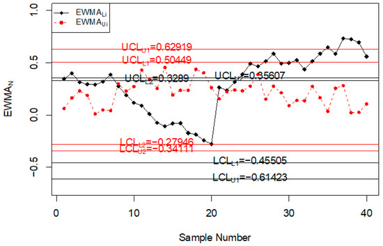
Figure 1.
Proposed control chart for simulated data set.
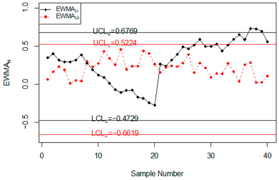
Figure 2.
The control chart by [33] for simulated data set.
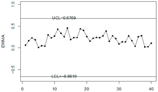
Figure 3.
The control chart by [39] for simulated data set.
5. Road Accidents and Injuries Monitoring Using Real Data
In this section, the application of the proposed control chart is given with the help of two real examples. The real data of injuries and accidents in Saudi Arabia were collected from https://data.gov.sa/Data/en/dataset/1439/resource/e6a973aa-32a8-4fa2-964c-78bcf0e8bf58 (accessed on 16 October 2020). The monitoring of road injuries using the proposed control chart and existing charts by [33,39] is discussed in example 1. Example 2 shows the control chart for monitoring the number of accidents using the proposed control chart and the existing control charts proposed by [33,39].
5.1. Example 1: Monitoring the Injuries
For the real-life application of the proposed chart, the injury data of various age ranges of people in different months of the year are reported in Table 8. The injury of people in various months of the year is a variable of interest here. The data are shown in Table 8. The calculations of the statistic of when and are also shown in Table 8.
Table 8.
Real data related to Injury Data of Jeddah.
The Injury level with the different age range in the whole year is shown in Figure 4. So, it can be seen that most people that are injured during road accidents are aged from 18 years to 30 years; less injury is recorded in people whose age is less than 18 years or more than 50 years. The application of the proposed control chart and the two existing charts is also shown using the control chart figures. The monitoring of road injuries using the proposed control chart is shown in Figure 5. The control chart proposed by [33] for the injuries data is shown in Figure 6. Figure 7 presents the control chart proposed by [39]. From Figure 6, it can be noted that some points are in indeterminate intervals and several points are near control limits which are indicating that there may be a shift in the injuries. On the other hand, Figure 6 and Figure 7 show that the number of injuries is within control, and these charts are not indicating any issue in the process. By comparing Figure 5 of the proposed chart with Figure 6 and Figure 7 of the existing control charts, it can be concluded that the proposed chart shows that the decision-makers can expect a shift in road injuries. Therefore, they should be alert and identify the factors for this shift in the process.
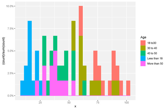
Figure 4.
A histogram represents the road accident Injury level with different age group.
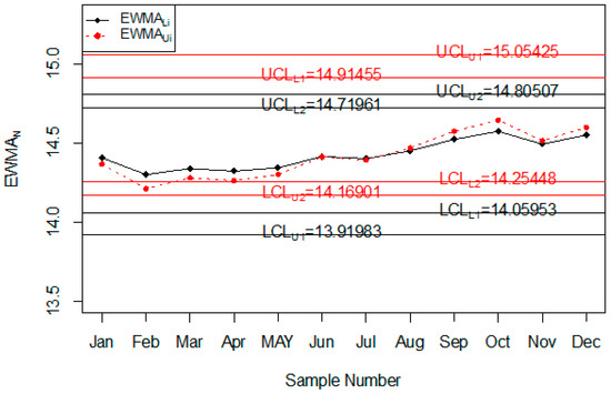
Figure 5.
The Proposed control chart for injuries data.
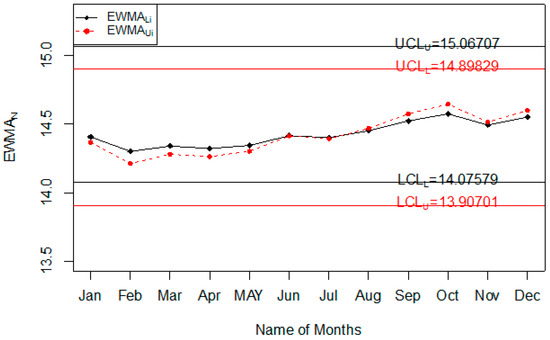
Figure 6.
Chart for injuries data.
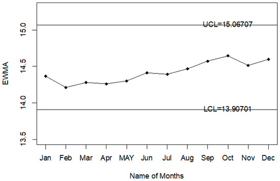
Figure 7.
Chart for injuries data.
5.2. Example 2: Monitoring Road Accidents
For the application of the proposed chart, the road accident data of all days and weeks of the year are used. The purpose of this example is to monitor road accidents on various days of the week. The data of road accidents are shown in Table 9. The values of the statistic of when and are also reported in Table 9. The application of the proposed control chart and two existing charts are also shown using the control chart Figures. The monitoring of road accidents using the proposed control chart is shown in Figure 8. The control chart proposed by [33] for road accidents data is shown in Figure 9. Figure 10 presents the control chart for road accidents proposed by [39]. From Figure 8, it can be noted that some points are in indeterminate intervals and several points are near control limits which are indicating that there may be a shift in road accidents. On the other hand, Figure 9 and Figure 10 show that the number of road accidents is within control, and these charts are not indicating any issue in the process. By comparing Figure 8 of the proposed chart with Figure 9 and Figure 10 of the existing control charts, it can be concluded that the proposed chart shows that the decision-makers can expect a shift in road accidents. Therefore, they should be alert and identify the factors that cause the shift in road accidents.
Table 9.
Accident Data in Jeddah.
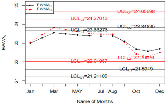
Figure 8.
The proposed control chart for accidents data.
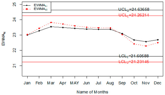
Figure 9.
Chart for accidents data [33].
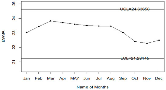
Figure 10.
Chart for accidents data set.
6. Concluding Remarks
The control chart for monitoring road accidents and road injuries when the smoothing constant is uncertain was presented in the paper. The operational procedure of the proposed chart was explained. The neutrosophic Monte Carlo simulation for the proposed control chart was introduced and used to present the Tables and control chart Figures. The comparative study showed that the proposed control chart is quite an effective tool in monitoring road accidents and road injuries. The efficiency of the proposed control chart was shown over two control charts in terms of NARL. Based on the analysis, it is recommended to apply the proposed control chart in monitoring highways and motorways to minimize road accidents and injuries. The proposed control chart using a cost model can be studied as future research. The proposed control chart using the rank set sampling scheme is also a fruitful area for future research. The seasonal trend of the series of accidents and injuries can be studied as future research.
Author Contributions
Conceptualization, M.A. (Muhammad Asalam) and M.A. (Mohammed Albassam); methodology, M.A. (Mohammed Albassam); software, M.A. (Muhammad Asalam); validation, M.A. (Muhammad Asalam) and M.A. (Mohammed Albassam). All authors have read and agreed to the published version of the manuscript.
Funding
This article was funded by the Deanship of Scientific Research (DSR) at King Abdulaziz University, Jeddah. The author therefore acknowledges DSR with thanks for technical and financial support.
Institutional Review Board Statement
Not applicable.
Informed Consent Statement
Not applicable.
Data Availability Statement
The data are given in the paper.
Conflicts of Interest
The authors declare no conflict of interest.
Appendix A
| #for laplace distribution need library (LaplacesDemon). |
| set.seed(5577) |
| rl<-c() |
| G<-c() |
| H<-c() |
| vt<-c() |
| var_SP<-c() |
| arl<-c() |
| n=7;Tk1=0.9165;mu.x=0.178;la=0.12;r0=370;a=-1.0827;b=2.8042;c=0.5678;Tk=0.00335 |
| k1=2.787 |
| k2=1.479 |
| shift<-c(1.00,1.05,1.10,1.15,1.2,1.25,1.3,1.4,1.50,1.6,1.7,1.8,1.9,2.00,2.25,2.50,3.00,4) |
| for(l in 1:length(shift)) |
| { |
| p1=shift[l] |
| for(j in 1:1000) |
| { |
| run=0 |
| rep=0 |
| for(i in 1:5000) |
| { |
| X=rnorm(n,0,1);X |
| sk=var(X);sk |
| x[i]=a+b*log(sk+c);x |
| var.x=var(x);var.x |
| ucl1=Tk+k1*sqrt((la/(2-la))*var.x);ucl1 |
| lcl1=Tk-k1*sqrt((la/(2-la))*var.x);lcl1 |
| ucl2=Tk+k2*sqrt((la/(2-la))*var.x);ucl2 |
| lcl2=Tk-k2*sqrt((la/(2-la))*var.x);lcl2 |
| #if (i==1){G[i]=la*SR[i])+(1-la)*mu.x}else{G[i])=la*SR[i]+(1-la)*G[i-1]} |
| if (i==1){H[i]=la*x[i]+(1-la)*mu.x} else{H[i]=la*x[i]+(1-la)*H[i-1]} |
| if(H[i]>ucl1|H[i]<lcl1){runs=i |
| break |
| } |
| if((H[i]>=lcl1 & H[i]<lcl2) | (H[i]>ucl2 & H[i]<=ucl1)){ |
| rep=rep+1; |
| } |
| } |
| if(runs>0) |
| rl[j]=runs-rep |
| } |
| } |
| arl=mean(rl) |
| SDRL=sd(rl) |
| MDRL=median(rl) |
| print(cbind(arl,SDRL)) |
References
- Irianto, D.; Juliani, A. A two control limits double sampling control chart by optimizing producer and customer risks. J. Eng. Technol. Sci. 2010, 42, 165–178. [Google Scholar] [CrossRef][Green Version]
- Abbas, N.; Saeed, U.; Riaz, M.; Abbasi, S.A. On designing an assorted control charting approach to monitor process dispersion: An application to hard-bake process. J. Taibah Univ. Sci. 2019, 14, 65–76. [Google Scholar] [CrossRef]
- Pokropp, F.; Seidel, W.; Begun, A.; Heidenreich, M.; Sever, K. Control Charts for the Number of Children Injured in Traffic Accidents Frontiers in Statistical Quality Control 8; Springer: Berlin/Heidelberg, Germany, 2006; pp. 151–171. [Google Scholar]
- Rębisz, B. The study of the dynamics of traffic accidents using the control charts. Mod. Manag. Rev. 2013, 18, 135–144. [Google Scholar] [CrossRef]
- Schuh, A.; Camelio, J.A.; Woodall, W.H. Control charts for accident frequency: A motivation for real-time occupational safety monitoring. Int. J. Inj. Control. Saf. Promot. 2013, 21, 154–162. [Google Scholar] [CrossRef] [PubMed]
- Baradaran, V.; Dashtbani, H. A decision support system for monitoring traffic by statistical control charts. Manag. Sci. Lett. 2014, 4, 1661–1670. [Google Scholar] [CrossRef]
- Mannering, F.L.; Shankar, V.; Bhat, C.R. Unobserved heterogeneity and the statistical analysis of highway accident data. Anal. Methods Accid. Res. 2016, 11, 1–16. [Google Scholar] [CrossRef]
- Olanrewaju, F.; Daniel, O.O.; Tajudeen, A.A. Comparative Analysis on EWMA and Poisson Cusum Chart in the Assessment of Road Traffic Crashes (RTC) in Osun State Nigeria. Am. J. Theor. Appl. Stat. 2017, 6, 95. [Google Scholar] [CrossRef][Green Version]
- Alogaili, A.; Mannering, F. Unobserved heterogeneity and the effects of driver nationality on crash injury severities in Saudi Arabia. Accid. Anal. Prev. 2020, 144, 105618. [Google Scholar] [CrossRef]
- Li, Q.; Li, X.; Mannering, F. A Statistical Study of Discretionary Lane-changing Decision with Heterogeneous Vehicle and Driver Characteristics. Transp. Res. Rec. 2020. [Google Scholar] [CrossRef]
- Stokes, R.W.; Mutabazi, M.I. Rate-quality control method of identifying hazardous road locations. Transp. Res. Rec. 1996, 1542, 44–48. [Google Scholar] [CrossRef]
- Mansuri, F.A.; Al-Zalabani, A.H.; Zalat, M.M.; Qabshawi, R.I. Road safety and road traffic accidents in Saudi Arabia: A systematic review of existing evidence. Saudi Med. J. 2015, 36, 418. [Google Scholar] [CrossRef] [PubMed]
- Alnawmasi, N.; Mannering, F. A statistical assessment of temporal instability in the factors determining motorcyclist injury severities. Anal. Methods Accid. Res. 2019, 22, 100090. [Google Scholar] [CrossRef]
- Tang, J.; Zheng, L.; Han, C.; Yin, W.; Zhang, Y.; Zou, Y.; Huang, H. Statistical and machine-learning methods for clearance time prediction of road incidents: A methodology review. Anal. Methods Accid. Res. 2020, 27, 100123. [Google Scholar] [CrossRef]
- Rissanen, R.; Ifver, J.; Hasselberg, M.; Berg, H.-Y. Quality of life following road traffic injury: The impact of age and gender. Qual. Life Res. 2020, 29, 1587–1596. [Google Scholar] [CrossRef] [PubMed]
- Islam, M.; Alnawmasi, N.; Mannering, F. Unobserved heterogeneity and temporal instability in the analysis of work-zone crash-injury severities. Anal. Methods Accid. Res. 2020, 28, 100130. [Google Scholar] [CrossRef]
- Smarandache, F. Introduction to neutrosophic statistics. Infin. Study 2014. [Google Scholar] [CrossRef]
- Smarandache, F.; Khalid, H.E. Neutrosophic precalculus and neutrosophic calculus. Infin. Study 2015. [Google Scholar] [CrossRef]
- Aslam, M. Monitoring the road traffic crashes using NEWMA chart and repetitive sampling. Int. J. Inj. Control. Saf. Promot. 2021, 28, 39–45. [Google Scholar] [CrossRef] [PubMed]
- Chen, J.; Ye, J.; Du, S. Scale Effect and Anisotropy Analyzed for Neutrosophic Numbers of Rock Joint Roughness Coefficient Based on Neutrosophic Statistics. Symmetry 2017, 9, 208. [Google Scholar] [CrossRef]
- Chen, J.; Ye, J.; Du, S.; Yong, R. Expressions of Rock Joint Roughness Coefficient Using Neutrosophic Interval Statistical Numbers. Symmetry 2017, 9, 123. [Google Scholar] [CrossRef]
- Aslam, M. A new method to analyze rock joint roughness coefficient based on neutrosophic statistics. Measurement 2019, 146, 65–71. [Google Scholar] [CrossRef]
- Kahraman, C.; Bozdag, C.E.; Ruan, D.; Ozok, A.F. Fuzzy sets approaches to statistical parametric and nonparametric tests. Int. J. Intell. Syst. 2004, 19, 1069–1087. [Google Scholar] [CrossRef]
- Grzegorzewski, P. k-sample median test for vague data. Int. J. Intell. Syst. 2009, 24, 529–539. [Google Scholar] [CrossRef]
- Shafiq, M.; Atif, M.; Viertl, R. Generalized Likelihood Ratio Test and Cox’sF-Test Based on Fuzzy Lifetime Data. Int. J. Intell. Syst. 2016, 32, 3–16. [Google Scholar] [CrossRef]
- Du, W.S. Correlation and correlation coefficient of generalized orthopair fuzzy sets. Int. J. Intell. Syst. 2019, 34, 564–583. [Google Scholar] [CrossRef]
- Grzegorzewski, P.; Śpiewak, M. The sign test and the signed-rank test for interval-valued data. Int. J. Intell. Syst. 2019, 34, 2122–2150. [Google Scholar] [CrossRef]
- Singh, S.; Ganie, A.H. On some correlation coefficients in Pythagorean fuzzy environment with applications. Int. J. Intell. Syst. 2020, 35, 682–717. [Google Scholar] [CrossRef]
- Flores, M.; Naya, S.; Fernández-Casal, R.; Zaragoza, S.; Raña, P.; Tarrío-Saavedra, J. Constructing a Control Chart Using Functional Data. Mathematics 2020, 8, 58. [Google Scholar] [CrossRef]
- Al-Marshadi, A.H.; Shafqat, A.; Aslam, M.; Alharbey, A. Performance of a New Time-Truncated Control Chart for Weibull Distribution Under Uncertainty. Int. J. Comput. Intell. Syst. 2021, 14, 1256. [Google Scholar] [CrossRef]
- Ajadi, J.O.; Wang, Z.; Zwetsloot, I.M. A review of dispersion control charts for multivariate individual observations. Qual. Eng. 2020, 1–16. [Google Scholar] [CrossRef]
- Aslam, M.; Al-Marshadi, A.H.; Khan, N. A New X-Bar Control Chart for Using Neutrosophic Exponentially Weighted Moving Average. Mathematics 2019, 7, 957. [Google Scholar] [CrossRef]
- Aslam, M.; Bantan, R.A.; Khan, N. Design of S2N—NEWMA Control Chart for Monitoring Process having Indeterminate Production Data. Processes 2019, 7, 742. [Google Scholar] [CrossRef]
- Sherman, R.E. Design and evaluation of a repetitive group sampling plan. Technometrics 1965, 7, 11–21. [Google Scholar] [CrossRef]
- Box, G.E.; Hunter, W.G.; Hunter, J.S. Statistics for Experimenters; John Wiley and Sons: New York, NY, USA, 1978. [Google Scholar]
- Crowder, S.V.; Hamilton, M.D. An EWMA for Monitoring a Process Standard Deviation. J. Qual. Technol. 1992, 24, 12–21. [Google Scholar] [CrossRef]
- Bissell, D.; Montgomery, D.C. Introduction to Statistical Quality Control. J. R. Stat. Soc. Ser. D 1986, 35, 81. [Google Scholar] [CrossRef]
- Johnsson, N.; Kotz, S.; Balakrishnan, N. Continuous Univariate Distributions; John Wiley and Sons: New York, NY, USA, 1994; Volume 1. [Google Scholar]
- Castagliola, P. A NewS2-EWMA Control Chart for Monitoring the Process Variance. Qual. Reliab. Eng. Int. 2005, 21, 781–794. [Google Scholar] [CrossRef]
Publisher’s Note: MDPI stays neutral with regard to jurisdictional claims in published maps and institutional affiliations. |
© 2021 by the authors. Licensee MDPI, Basel, Switzerland. This article is an open access article distributed under the terms and conditions of the Creative Commons Attribution (CC BY) license (https://creativecommons.org/licenses/by/4.0/).