Simulating Urban Growth Scenarios Based on Ecological Security Pattern: A Case Study in Quanzhou, China


Abstract
1. Introduction
2. Study Context and Data Sources
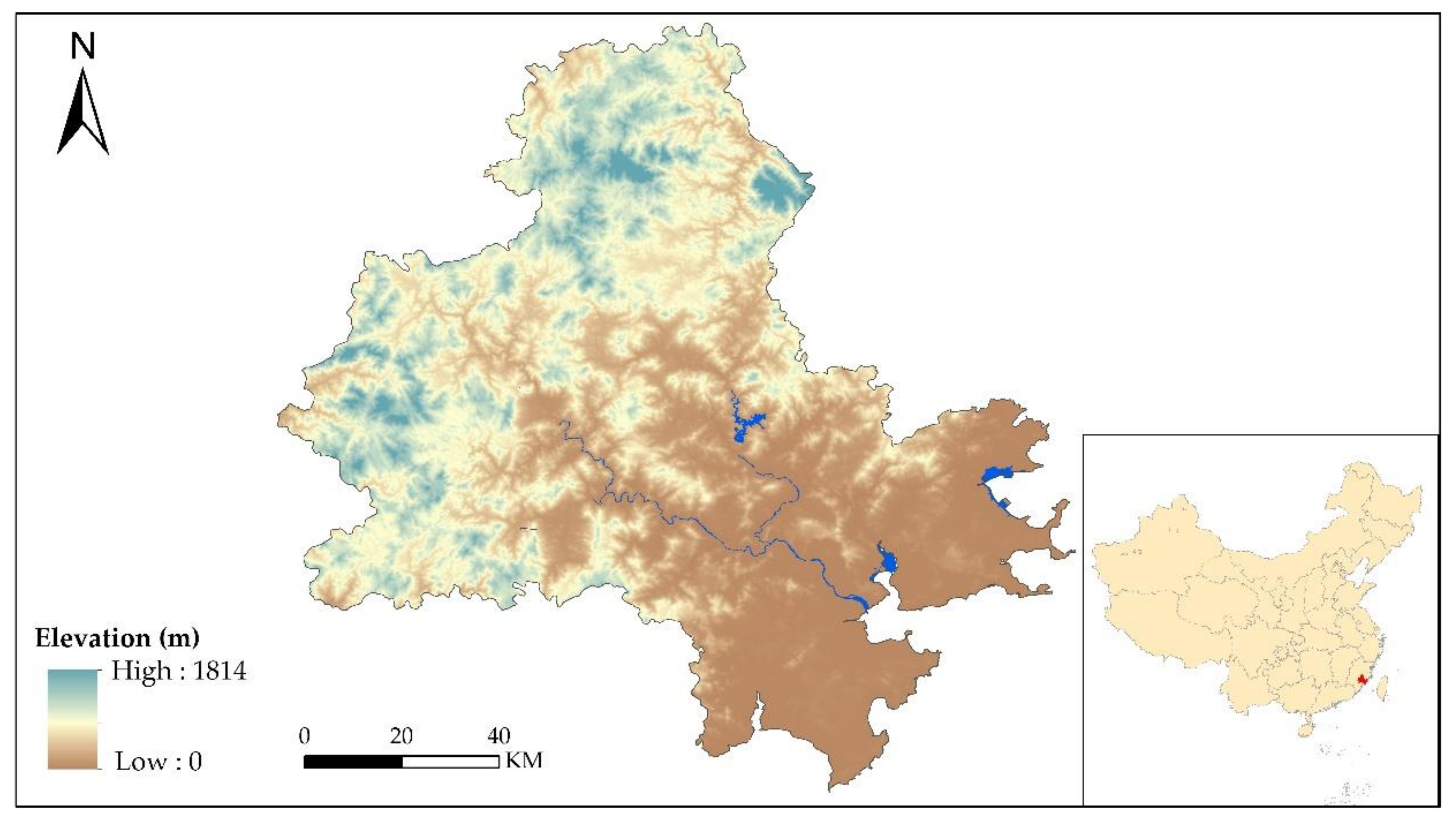
2.1. Study Context
2.2. Data
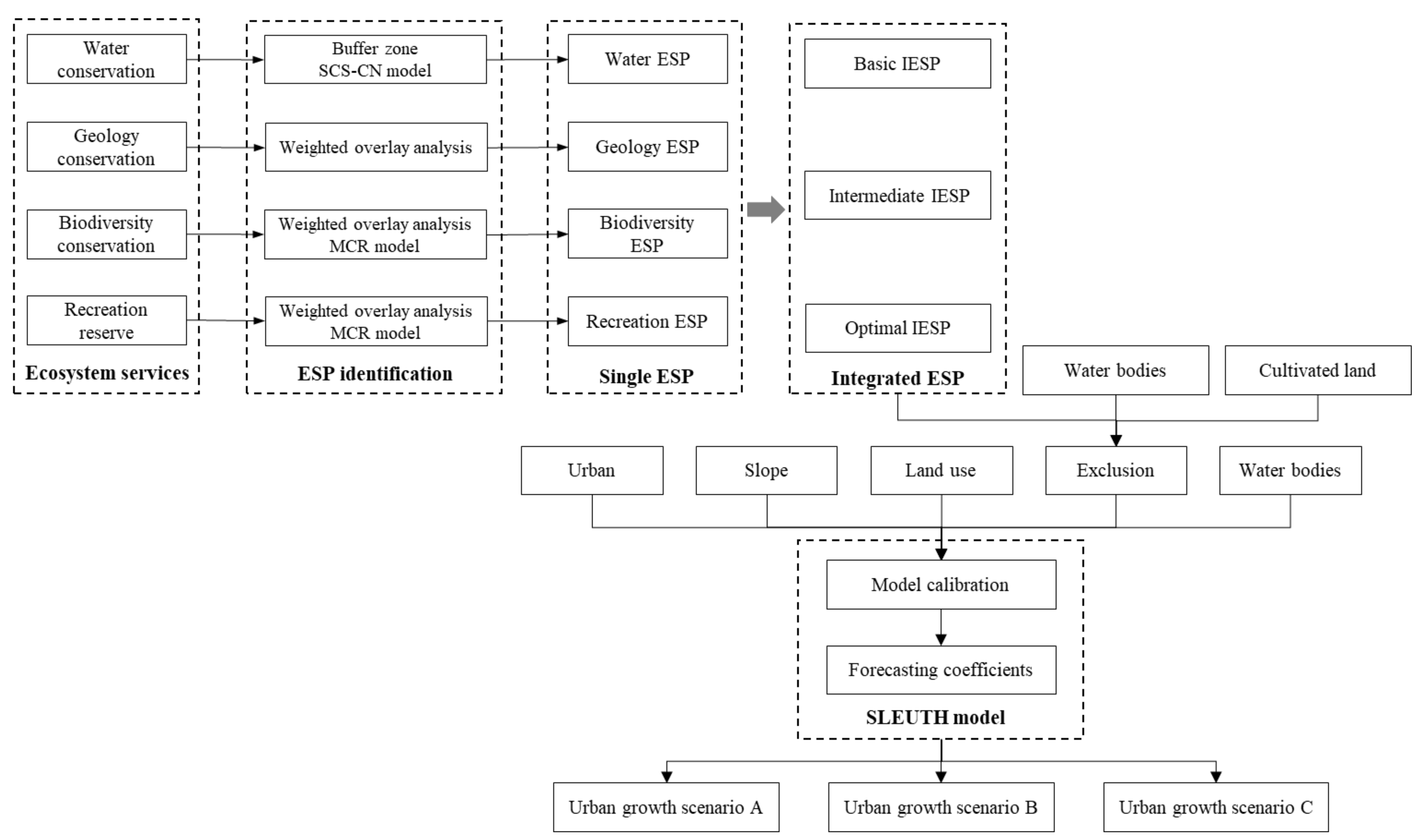
3. Methodology
3.1. ESP Identification and Construction
3.1.1. Overlay Analysis
3.1.2. Soil Conservation Service Curve Number (SCS-CN) Model
3.1.3. Minimum Cumulative Resistance (MCR) model
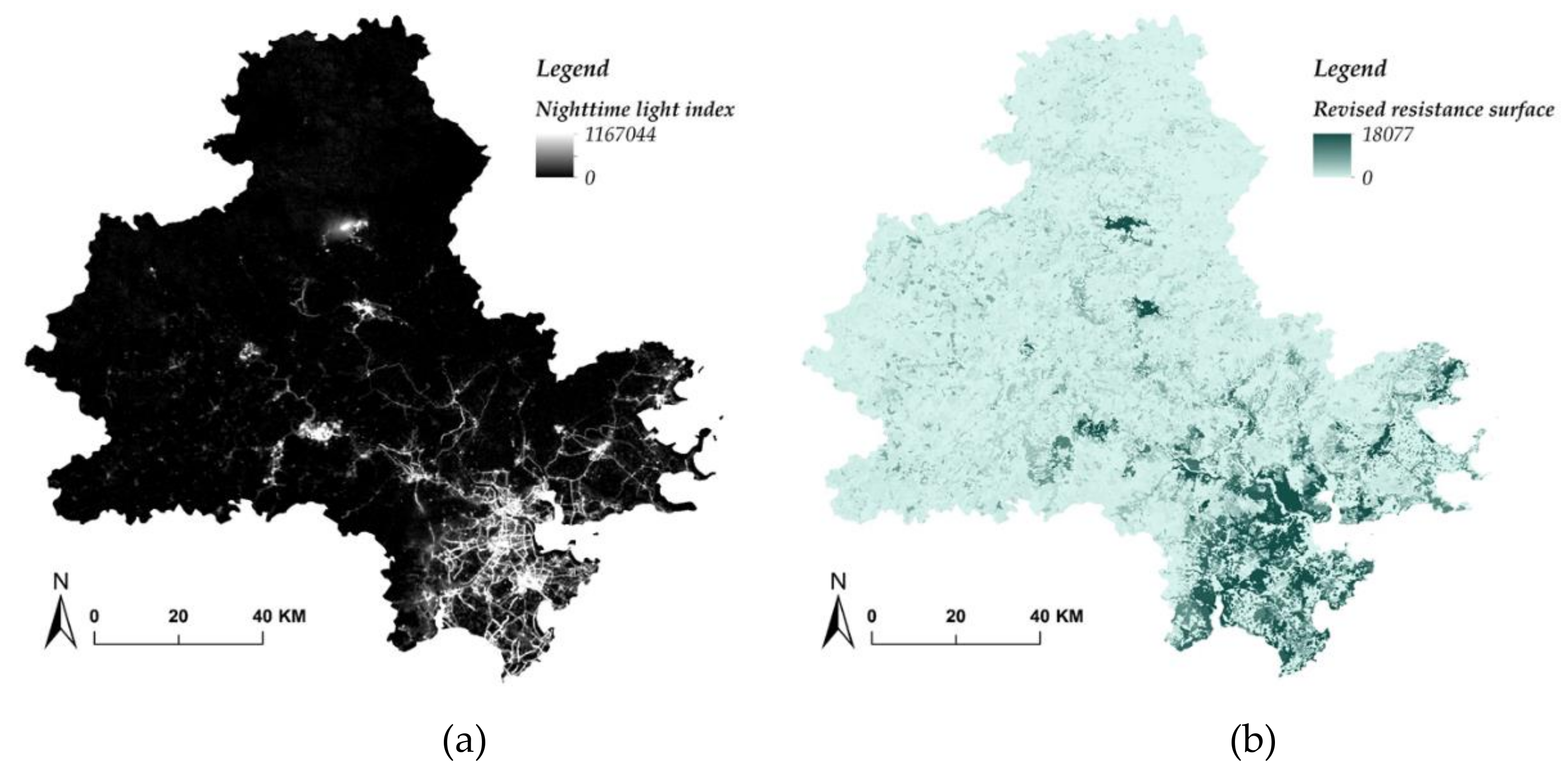
3.1.4. Resistance Surface Revision
3.1.5. Integrated ESP Construction
3.2. SLEUTH Model Calibration
4. Results
4.1. ESP Identification and Construction
4.1.1. Water ESP Identification
4.1.2. Geology ESP Identification
4.1.3. Biodiversity ESP Identification
4.1.4. Recreation ESP Identification
4.1.5. Integrated ESP Identification
4.2. Urban Growth Modeling Results
5. Discussion
6. Conclusions
Author Contributions
Funding
Conflicts of Interest
References
- Peng, J.; Pan, Y.; Liu, Y.; Zhao, H.; Wang, Y. Linking ecological degradation risk to identify ecological security patterns in a rapidly urbanizing landscape. Habitat Int. 2018, 71, 110–124. [Google Scholar] [CrossRef]
- Peng, J.; Yang, Y.; Liu, Y.; Du, Y.; Meersmans, J.; Qiu, S. Linking ecosystem services and circuit theory to identify ecological security patterns. Sci. Total Environ. 2018, 644, 781–790. [Google Scholar] [CrossRef] [PubMed]
- Guo, R.; Wu, T.; Liu, M.; Huang, M.; Stendardo, L.; Zhang, Y. The Construction and Optimization of Ecological Security Pattern in the Harbin-Changchun Urban Agglomeration, China. Int. J. Environ. Res. Public Health 2019, 16, 1190. [Google Scholar] [CrossRef] [PubMed]
- Fu, Y.; Shi, X.; He, J.; Yuan, Y.; Qu, L. Identification and optimization strategy of county ecological security pattern: A case study in the Loess Plateau, China. Ecol. Indic. 2020, 112, 106030. [Google Scholar] [CrossRef]
- Li, J.L.; Xu, J.G.; Chu, J.L. The Construction of a Regional Ecological Security Pattern Based on Circuit Theory. Sustainability 2019, 11, 6343. [Google Scholar] [CrossRef]
- Guo, S.S.; Wang, Y.H. Ecological Security Assessment Based on Ecological Footprint Approach in Hulunbeir Grassland, China. Int. J. Environ. Res. Public Health 2019, 16, 4805. [Google Scholar] [CrossRef]
- Wang, Y.; Pan, J. Building ecological security patterns based on ecosystem services value reconstruction in an arid inland basin: A case study in Ganzhou District, NW China. J. Clean. Prod. 2019, 241, 118337. [Google Scholar] [CrossRef]
- Hu, M.; Li, Z.; Yuan, M.; Fan, C.; Xia, B. Spatial differentiation of ecological security and differentiated management of ecological conservation in the Pearl River Delta, China. Ecol. Indic. 2019, 104, 439–448. [Google Scholar] [CrossRef]
- Hodson, M.; Marvin, S. ‘Urban Ecological Security’: A New Urban Paradigm? Int. J. Urban Reg. Res. 2009, 33, 193–215. [Google Scholar] [CrossRef]
- Peng, J.; Zhao, H.; Liu, Y. Urban ecological corridors construction: A review. Acta Ecol. Sin. 2017, 37, 23–30. [Google Scholar] [CrossRef]
- Liu, D.; Chang, Q. Ecological security research progress in China. Acta Ecol. Sin. 2015, 35, 111–121. [Google Scholar] [CrossRef]
- Wang, C.; Yu, C.; Chen, T.; Feng, Z.; Hu, Y.; Wu, K. Can the establishment of ecological security patterns improve ecological protection? An example of Nanchang, China. Sci. Total Environ. 2020, 740, 140051. [Google Scholar] [CrossRef] [PubMed]
- Ezeonu, I.C.; Ezeonu, F.C. The environment and global security. Environmentalist 2000, 20, 41–48. [Google Scholar] [CrossRef]
- Pirages, D. Ecological security: Micro-threats to human well-being. In People and Their Planet; Springer: Berlin/Heidelberg, Germany, 1999; pp. 284–298. [Google Scholar]
- Lu, S.; Li, J.; Guan, X.; Gao, X.; Gu, Y.; Zhang, D.; Mi, F.; Li, D. The evaluation of forestry ecological security in China: Developing a decision support system. Ecol. Indic. 2018, 91, 664–678. [Google Scholar] [CrossRef]
- Yu, G.; Zhang, S.; Yu, Q.; Fan, Y.; Zeng, Q.; Wu, L.; Zhou, R.; Nan, N.; Zhao, P. Assessing ecological security at the watershed scale based on RS/GIS: A case study from the Hanjiang River Basin. Stoch. Environ. Res. Risk Assess. 2014, 28, 307–318. [Google Scholar] [CrossRef]
- Lu, S.; Tang, X.; Guan, X.; Qin, F.; Liu, X.; Zhang, D. The assessment of forest ecological security and its determining indicators: A case study of the Yangtze River Economic Belt in China. J. Environ. Manag. 2020, 258, 110048. [Google Scholar] [CrossRef]
- Wu, X.; Liu, S.; Sun, Y.; An, Y.; Dong, S.; Liu, G. Ecological security evaluation based on entropy matter-element model: A case study of Kunming city, southwest China. Ecol. Indic. 2019, 102, 469–478. [Google Scholar] [CrossRef]
- Xu, J.Y.; Fan, F.; Liu, Y.; Dong, J.; Chen, J. Construction of Ecological Security Patterns in Nature Reserves Based on Ecosystem Services and Circuit Theory: A Case Study in Wenchuan, China. Int. J. Environ. Res. Public Health 2019, 16, 3220. [Google Scholar] [CrossRef]
- Gebler, D.; Wiegleb, G.; Szoszkiewicz, K. Integrating river hydromorphology and water quality into ecological status modelling by artificial neural networks. Water Res. 2018, 139, 395–405. [Google Scholar] [CrossRef]
- Wang, Q.; Li, S.; He, G.; Li, R.; Wang, X. Evaluating sustainability of water-energy-food (WEF) nexus using an improved matter-element extension model: A case study of China. J. Clean. Prod. 2018, 202, 1097–1106. [Google Scholar] [CrossRef]
- Gao, P.P.; Li, Y.P.; Sun, J.; Li, H.W. Coupling fuzzy multiple attribute decision-making with analytic hierarchy process to evaluate urban ecological security: A case study of Guangzhou, China. Ecol. Complex. 2018, 34, 23–34. [Google Scholar] [CrossRef]
- Zhou, Y.; Varquez, A.C.G.; Kanda, M. High-resolution global urban growth projection based on multiple applications of the SLEUTH urban growth model. Sci. Data 2019, 6, 34. [Google Scholar] [CrossRef] [PubMed]
- Feng, H.H.; Liu, H.P.; Lu, Y. Scenario Prediction and Analysis of Urban Growth Using SLEUTH Model. Pedosphere 2012, 22, 206–216. [Google Scholar] [CrossRef]
- Chaudhuri, G.; Clarke, K.C. Modeling an Indian megalopolis-A case study on adapting SLEUTH urban growth model. Comput. Environ. Urban Syst. 2019, 77, 101358. [Google Scholar] [CrossRef]
- Chaudhuri, G.; Clarke, K. The SLEUTH land use change model: A review. Environ. Resour. Res. 2013, 1, 88–105. [Google Scholar]
- Jantz, C.A.; Goetz, S.J.; Shelley, M.K. Using the Sleuth Urban Growth Model to Simulate the Impacts of Future Policy Scenarios on Urban Land Use in the Baltimore-Washington Metropolitan Area. Environ. Plan. B Plan. Des. 2004, 31, 251–271. [Google Scholar] [CrossRef]
- Saxena, A.; Jat, M.K. Capturing heterogeneous urban growth using SLEUTH model. Remote Sens. Appl. Soc. Environ. 2019, 13, 426–434. [Google Scholar] [CrossRef]
- Saxena, A.; Jat, M.K. Land suitability and urban growth modeling: Development of SLEUTH-Suitability. Comput. Environ. Urban Syst. 2020, 81, 101475. [Google Scholar] [CrossRef]
- Fujian Provincial Bureau of Statistics. Fujian Statistical Yearbook 2019; Fujian Provincial Bureau of Statistics: Fujian, China, 2019.
- Xiao, B.; Wang, Q.-H.; Fan, J.; Han, F.-P.; Dai, Q.-H. Application of the SCS-CN Model to Runoff Estimation in a Small Watershed with High Spatial Heterogeneity. Pedosphere 2011, 21, 738–749. [Google Scholar] [CrossRef]
- Liu, J.X.; Zhang, G.; Zhuang, Z.; Cheng, Q.; Gao, Y.; Chen, T.; Huang, Q.; Xu, L.; Chen, D. A new perspective for urban development boundary delineation based on SLEUTH-InVEST model. Habitat Int. 2017, 70, 13–23. [Google Scholar] [CrossRef]
- Terando, A.J.; Costanza, J.; Belyea, C.; Dunn, R.R.; McKerrow, A.; Collazo, J.A. The Southern Megalopolis: Using the Past to Predict the Future of Urban Sprawl in the Southeast U.S. PLoS ONE 2014, 9, e102261. [Google Scholar] [CrossRef] [PubMed]
- Kong, F.; Yin, H.; Nakagoshi, N.; Zong, Y. Urban green space network development for biodiversity conservation: Identification based on graph theory and gravity modeling. Landsc. Urban Plan. 2010, 95, 16–27. [Google Scholar] [CrossRef]
- Zhang, K.H.; Song, S. Rural–urban migration and urbanization in China: Evidence from time-series and cross-section analyses. China Econ. Rev. 2003, 14, 386–400. [Google Scholar] [CrossRef]
- Yu, Z.; Fryd, O.; Sun, R.; Jørgensen, G.; Yang, G.; Özdil, N.C.; Vejre, H. Where and how to cool? An idealized urban thermal security pattern model. Landsc. Ecol. 2020. [Google Scholar] [CrossRef]


| Data | Utility | Data Source |
|---|---|---|
| Land use | ESP identification; Urban growth simulation | Resource and Environment Cloud Platform http://www.resdc.cn/ |
| Annual rainfall | Water & Geology ESP identification | National Meteorological Information Center http://data.cma.cn/; Local weather station records |
| NDVI | Biodiversity & Geology ESP identification | U.S. Geological Survey Landsat image |
| Slope | Water & Geology & Biodiversity ESP identification; Urban growth simulation | Calculated from DEM data; Geospatial Data Cloud https://www.gscloud.cn/ |
| Elevation | Water & Geology & Biodiversity ESP identification | Derived from DEM data; Geospatial Data Cloud https://www.gscloud.cn/ |
| Curvature | Geology ESP identification | Calculated from DEM data; Geospatial Data Cloud https://www.gscloud.cn/ |
| Hill-shade | Urban growth simulation | Calculated from DEM data; Geospatial Data Cloud https://www.gscloud.cn/ |
| Road | Geology & Biodiversity ESP identification; Urban growth simulation | National Geoinformation Service http://www.webmap.cn |
| Geological hazards | Geology ESP identification | Fujian Seismological Bureau; Fujian Water Conservancy Bureau |
| Soil type | Geology ESP identification | Fujian Agriculture Department |
| Nighttime light | Biodiversity ESP revision | Luojia-1 Satellite image http://www.hbeos.org.cn |
| Recreation resources | Recreation ESP identification | Ministry of Ecology and Environment of China; Fujian Forestry Bureau |
| Growth Coefficients | Coarse | Fine | Final | BFC | |||
|---|---|---|---|---|---|---|---|
| MCI = 5 | MCI = 7 | MCI = 9 | |||||
| NI = 3163 | NI = 7851 | NI = 7796 | |||||
| OSM = 0.4679 | OSM = 0.4723 | OSM = 0.5034 | |||||
| Range | Step | Range | Step | Range | Step | ||
| Dispersion | 0–100 | 25 | 25–100 | 15 | 40–75 | 7 | 81 |
| Breed | 0–100 | 25 | 50–100 | 10 | 50–75 | 5 | 51 |
| Road gravity | 0–100 | 25 | 0–75 | 15 | 30–75 | 9 | 66 |
| Slope | 0–100 | 25 | 25–70 | 9 | 25–40 | 3 | 35 |
| Spread | 0–100 | 25 | 25–100 | 15 | 25–55 | 6 | 42 |
| Modelling Results | 2005 | 2010 | 2015 |
|---|---|---|---|
| Actual value (number of pixels) | 64,455 | 106,264 | 127,652 |
| Simulation value (number of pixels) | 56,427 | 94,628 | 11,6457 |
| Simulation accuracy (%) | 87.54 | 89.05 | 91.23 |
| Exclusion Layers | Urban Growth Scenario A | Urban Growth Scenario B | Urban Growth Scenario C |
|---|---|---|---|
| Built–up area in 2015 | 0 | 0 | 0 |
| Water body | 100 | 100 | 100 |
| Cultivated land | 100 | 100 | 100 |
| Basic IESP | 100 | 100 | 100 |
| Intermediate IESP | 70 | 70 | 0 |
| Optimal IESP | 50 | 0 | 0 |
| Evaluation Factor | Basic Water ESP | Intermediate Water ESP | Optimal Water ESP |
|---|---|---|---|
| Distance to river and lake (m) | ≤50 | 50–150 | 150–500 |
| Distance to surface water (m) | ≤500 | 500–1000 | 1000–1500 |
| Flood storage area (m3) | 3rd level of water storage area | 2nd level of water storage area | 1st level of water storage area |
| Distance to inundation area (km2) | 10–Year rain event | 50–Year rain event | 1000–Year rain event |
| Evaluation Factor | Standardized Value | Weight | ||||
|---|---|---|---|---|---|---|
| No Impact Area | Optimal ESP | Intermediate ESP | Basic Security Pattern | |||
| Insensitive (1) | Mildly Sensitive (3) | Moderately Sensitive (5) | Sensitive (7) | Highly Sensitive (9) | ||
| Average annual rainfall (mm) | <1300 | 1300–1400 | 1400–1500 | 1500–1600 | >1600 | 0.15 |
| Slope (°) | <5 | 5–15 | 15–25 | 25–35 | >35 | 0.1 |
| Elevation (m) | <200 | 200–500 | 500–800 | 800–1000 | >1000 | 0.1 |
| Curvature | −0.5–0.5 | (−1.5, −0.5], [0.5–1.5) | (−2.5, −1.5], [1.5–2.5) | (−3.5, −2.5], [2.5–3.5) | (−∞,−3.5], [3.5, ∞) | 0.1 |
| Soil type | Paddy soil Calcareous soil | Saline soil Sandy soil Meadow soil Limestone soil | Lateritic soil | Yellow soil Yellow–red soil Rhogosol Lithosol | Purple soil | 0.1 |
| Normalized difference vegetation index (NDVI) | <0.55 | 0.4–0.55 | 0.25–0.4 | 0.1–0.25 | <0.1 | 0.1 |
| Land cover | Construction land Waterbody Wetland | Forest Natural grassland Improved grassland | Irrigable land Dryland Garden plot | Artificial grassland Wild grassland Saline–alkali land | Slash land Bare land Sandy land Gravel land | 0.1 |
| Distance to major road (m) | >5000 | 3000–5000 | 1500–3000 | 500–1500 | <500 | 0.1 |
| Geological hazards number (per 25 km2) | <2 | 2–4 | 4–6 | 6–8 | >8 | 0.15 |
| Evaluation Factor | Classification | Value | Weight |
|---|---|---|---|
| Land cover | Urban and other construction lands | 0 | 0.35 |
| Rural residential land | 1 | ||
| Bare land | 2 | ||
| Lowly covered grassland | 3 | ||
| Dryland and medium covered grassland | 5 | ||
| Sparse forest and waterway | 6 | ||
| Shrub and highly covered grassland | 7 | ||
| Closed forest, lake, reservoir, wetland | 8 | ||
| Paddy filed and mudflats | 10 | ||
| Elevation (m) | 0–100 | 5 | 0.10 |
| 100–800 | 10 | ||
| 800–1500 | 5 | ||
| >1500 | 1 | ||
| Distance to water sources (m) | 0–2000 | 6 | 0.25 |
| 2000–7000 | 8 | ||
| 7000–15000 | 10 | ||
| 15000–30000 | 5 | ||
| >30000 | 2 | ||
| Distance to Built–up area (m) | >6000 | 10 | 0.15 |
| 4000–6000 | 5 | ||
| 2000–4000 | 3 | ||
| 0–2000 | 1 | ||
| 0 | 0 | ||
| Distance to road (m) | 0–500 | 0 | 0.15 |
| 500–1000 | 1 | ||
| 1000–2000 | 3 | ||
| 2000–4000 | 5 | ||
| >4000 | 10 |
| Land Cover | Resistance Coefficient | Land Cover | Resistance Coefficient |
|---|---|---|---|
| Closed forest | 1 | Mudflats | 100 |
| Shrub forest, highly covered grassland | 10 | Dryland | 200 |
| Medium covered grassland | 20 | Bare land and saline–alkali land | 300 |
| Sparse forest | 30 | Rural residential land | 400 |
| Paddy field | 50 | Urban land | 500 |
| Waterbody | 50 | Other construction lands | 500 |
| Evaluation Factor | Basic Biodiversity ESP | Intermediate Biodiversity ESP | Optimal Biodiversity ESP |
|---|---|---|---|
| Distance to biodiversity source (m) | 0 | 0–200 | 200–300 |
| MCR value | Level 1 | Level 2 | Level 3 |
| Distance to biodiversity corridor (m) | <100 | 100–200 | 200–300 |
| Evaluation Factor | Basic Recreation ESP | Intermediate Recreation ESP | Optimal Recreation ESP |
|---|---|---|---|
| Distance to recreation source (m) | 0 | 0–200 | 200–300 |
| MCR value | Level 1 | Level 2 | Level 3 |
| Distance to recreation corridor (m) | <100 | 100–200 | 200–300 |
| Period | Urban Growth Scenarios | Urban Growth Area (km2) | Annual Urban Growth Rate (%) |
|---|---|---|---|
| 2000–2015 | Historical record | 538.8 | 4.4% |
| 2015–2030 | Urban growth scenario A | 750.5 | 3.6% |
| Urban growth scenario B | 677.7 | 3.3% | |
| Urban growth scenario C | 498.4 | 2.5% |
© 2020 by the authors. Licensee MDPI, Basel, Switzerland. This article is an open access article distributed under the terms and conditions of the Creative Commons Attribution (CC BY) license (http://creativecommons.org/licenses/by/4.0/).
Share and Cite
Liu, X.; Wei, M.; Zeng, J. Simulating Urban Growth Scenarios Based on Ecological Security Pattern: A Case Study in Quanzhou, China. Int. J. Environ. Res. Public Health 2020, 17, 7282. https://doi.org/10.3390/ijerph17197282
Liu X, Wei M, Zeng J. Simulating Urban Growth Scenarios Based on Ecological Security Pattern: A Case Study in Quanzhou, China. International Journal of Environmental Research and Public Health. 2020; 17(19):7282. https://doi.org/10.3390/ijerph17197282
Chicago/Turabian StyleLiu, Xiaoyang, Ming Wei, and Jian Zeng. 2020. "Simulating Urban Growth Scenarios Based on Ecological Security Pattern: A Case Study in Quanzhou, China" International Journal of Environmental Research and Public Health 17, no. 19: 7282. https://doi.org/10.3390/ijerph17197282
APA StyleLiu, X., Wei, M., & Zeng, J. (2020). Simulating Urban Growth Scenarios Based on Ecological Security Pattern: A Case Study in Quanzhou, China. International Journal of Environmental Research and Public Health, 17(19), 7282. https://doi.org/10.3390/ijerph17197282