Dynamic Model for the Epidemiology of Diarrhea and Simulation Considering Multiple Disease Carriers


Abstract
1. Introduction
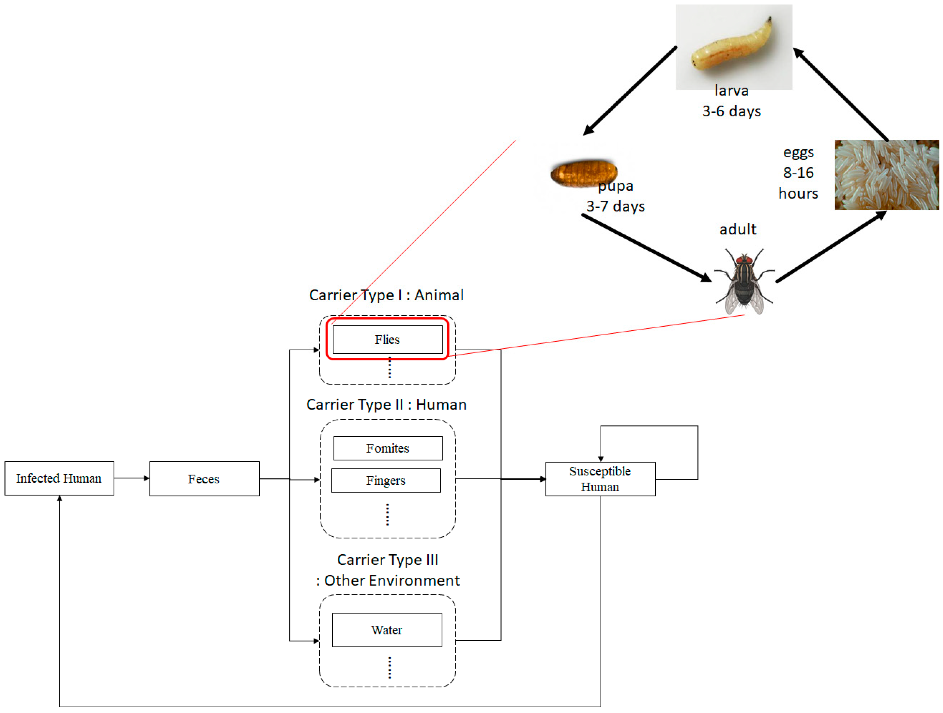
2. Background and Epidemiologic Network Model
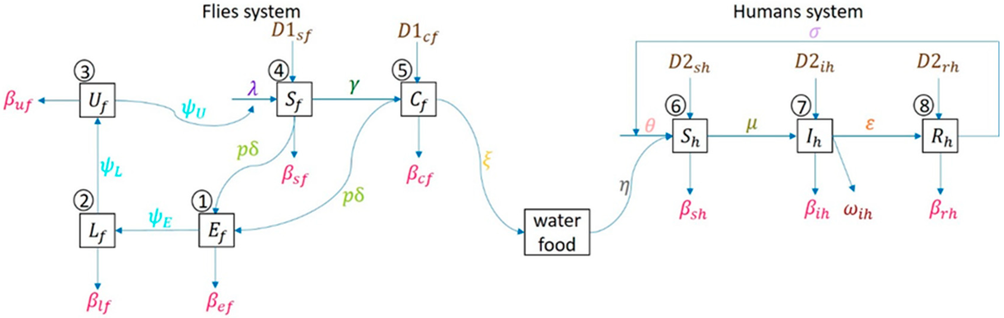
3. Epidemic Model Dynamics
4. Effective Control Framework Considering Multiple Disease Carriers
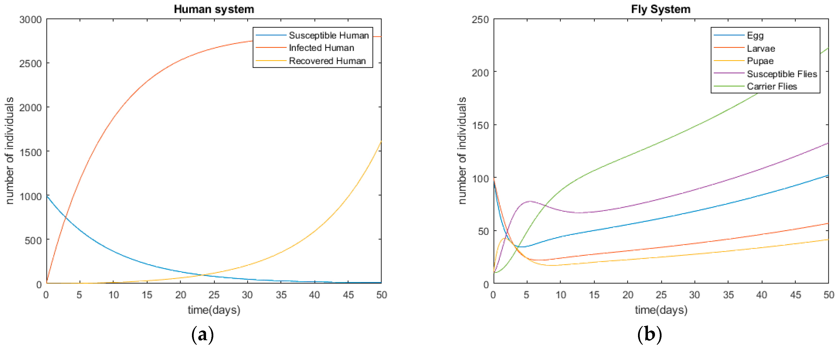
5. Simulation and Analysis of Control Model Considering Multiple Disease Carriers
6. Conclusions
Author Contributions
Funding
Conflicts of Interest
Appendix A
Appendix B
References
- GBD 2016 Causes of Death Collaborators. Global, regional, and national age-sex specific mortality for 264 causes of death, 1980–2016: A systematic analysis for the Global Burden of Disease Study 2016. Lancet 2017, 390, 1151–1210. [Google Scholar] [CrossRef]
- InformedHealth.org. Cologne, Germany: Institute for Quality and Efficiency in Health Care (IQWiG). 2006. Acute infectious Diarrhea: Common Germs and Routes of Infection. 4 May 2016. Available online: https://www.ncbi.nlm.nih.gov/books/NBK373086/ (accessed on 13 June 2019).
- Olsen, A.R.; Hammack, T.S. Isolation of Salmonella spp. from the housefly, Musca domestica L., and the dump fly, Hydrotaea aenescens (Wiedemann) (Diptera: Muscidae), at caged-layer houses. J. Food Prot. 2000, 63, 958–960. [Google Scholar] [CrossRef] [PubMed]
- Hosseini, S.M.; Zeyni, B.; Rastyani, S.; Jafari, R.; Shamloo, F.; Tabar, Z.K.; Rabestani, M.R. Presence of virulence factors and antibiotic resistances in Enterococcus sp collected from dairy products and meat. Der Pharm. Lett. 2016, 8, 138–145. [Google Scholar]
- Tsagaan, A.; Kanuka, I.; Okado, K. Study of pathogenic bacteria detected in fly samples using universal primer-multiplex PCR. Mong. J. Agric. Sci. 2015, 15, 27–32. [Google Scholar] [CrossRef]
- Nassiri, H.; Zarrin, M.; Veys-Behbahani, R.; Faramarzi, S.; Nasiri, A. Isolation and identification of pathogenic filamentous fungi and yeasts from adult house fly (Diptera: Muscidae) captured from the hospital environments in Alivaz city, Southwestern Iran. J. Med. Entomol. 2015, 52, 1351–1356. [Google Scholar]
- Peffly, R.L. A summary of recent studies on house flies in Egypt. J. Egypt. Public Health Assoc. 1953, 28, 55–74. [Google Scholar]
- Chavasse, D.C.; Shier, R.P.; Murphy, O.A.; Huttly, S.R.; Cousens, S.N.; Akhtar, A. Impact of fly control on childhood diarrhea in Pakistan: Community randomized trial. Lancet 1999, 353, 22–25. [Google Scholar] [CrossRef]
- Echeverria, P.; Harrison, B.A.; Tirapat, C.; McFarland, A. Flies as a source of enteric pathogens in a rural village in Thailand. Appl. Environ. Microbiol. 1983, 46, 32–36. [Google Scholar] [CrossRef]
- Nash, J.T. House flies as carriers of disease. J. Hyg. (Lond.) 1909, 9, 141–169. [Google Scholar] [CrossRef][Green Version]
- Collinet-Adler, S.; Babji, S.; Francis, M.; Kattula, D.; Premkumar, P.S.; Sarkar, R.; Mohan, V.R.; Ward, H.; Kang, G.; Balraj, V.; et al. Environmental Factors Associated with High Fly Densities and Diarrhea in Vellore, India. Appl. Environ. Microbiol. 2015, 81, 6053–6058. [Google Scholar] [CrossRef]
- Das, J.K.; Hadi, Y.B.; Salam, R.A.; Hoda, M.; Lassi, Z.S.; Bhutta, Z.A. Fly control to prevent diarrhea in children. Cochrane Database Syst. Rev. 2018, 12, CD011654. [Google Scholar] [PubMed]
- Cohen, D.; Green, M.; Block, C.; Slepon, R.; Ambar, R.; Wasserman, S.S.; Levine, M.M. Reduction of transmission of shigellosis by control of houseflies (Musca domestica). Lancet 1991, 337, 993–997. [Google Scholar] [CrossRef]
- Lindsay, D.; Stewart, W.; Watt, J. Effect of fly control on diarrhea in an area of moderate morbidity. Public Health Rep. 1953, 68, 361–367. [Google Scholar] [CrossRef] [PubMed]
- Watt, J.; Lindsay, D.R. Diarrhea control studies; effect of fly control in a high morbidity area. Public Health Rep. 1948, 63, 1319–1333. [Google Scholar] [CrossRef] [PubMed]
- Hartemink, N.; Vanwambeke, S.O.; Heesterbeek, H.; Rogers, D.; Morley, D.; Pesson, B.; Davies, C.; Mahamdallie, S.; Ready, P. Integrated mapping of establishment risk for emerging vector-borne infections: A case study of canine leishmaniasis in southwest France. PLoS ONE 2011, 6, e20817. [Google Scholar] [CrossRef] [PubMed]
- Lenhart, S.; Workman, J.T. Optimal Control Applied to Biological Models; Chapman and Hall/CRC: London, UK, 2007. [Google Scholar]
- Heffernan, J.; Smith, R.; Wahl, L. Perspectives on the basic reproductive ratio. J. R. Soc. Interface 2005, 2, 281–293. [Google Scholar] [CrossRef]
- Diekmann, O.; Heesterbeek, J.; Metz, J.A. On the definition and the computation of the basic reproduction ratio R0 in models for infectious diseases in heterogeneous populations. J. Math. Biol. 1990, 28, 365–382. [Google Scholar] [CrossRef]
- Pontryagin, L.S. Mathematical Theory of Optimal Processes; Routledge: London, UK, 2018. [Google Scholar]
- Getachew, T.T.; Oluwole, D.M.; David, M. Modelling and optimal control of pneumonia disease with cost-effective strategies. J. Biol. Dyn. 2017, 11 (Suppl. 2), 400–426. [Google Scholar]
- Cairncross, S.; Hunt, C.; Boisson, S.; Bostoen, K.; Curtis, V.; Fung, I.C.H.; Schmidt, W.-P. Water, sanitation and hygiene for the prevention of diarrhea. Int. J. Epidemiol. 2010, 39 (Suppl. 1), i193–i205. [Google Scholar] [CrossRef]
- Branz, A.; Levine, M.; Lehmann, L.; Bastable, A.; Ali, S.I.; Kadir, K.; Yates, T.; Bloom, D.; Lantagne, D. Chlorination of drinking water in emergencies: A review of knowledge, recommendations for implementation, and research needed. Waterlines 2017, 36, 4–39. [Google Scholar] [CrossRef]
- Okosun, K.O.; Rachid, O.; Marcus, N. Optimal control strategies and cost-effectiveness analysis of a malaria model. BioSystems 2013, 111, 83–101. [Google Scholar] [CrossRef] [PubMed]
- Fleming, W.H.; Rishel, R.W. Deterministic and Stochastic Optimal Control; Springer: New York, NY, USA, 2017. [Google Scholar]
- How Much Does It Cost to Get Rid Of Flies? Available online: https://www.kompareit.com/homeandgarden/home-services-compare-fly-exterminator-cost.html (accessed on 3 August 2020).
- Sandy, C.; Vivian, V. Water supply, sanitation and hygiene promotion. In Disease Control Priorities in Developing Countries; Oxford University Press: New York, NY, USA, 2006. [Google Scholar]
- Golan, E.H.; Vogel, S.J.; Frenzen, P.D.; Ralston, K.L. Tracing the Costs and Benefits of Improvements in Food Safety: The Case of the Hazard Analysis and Critical Control Point Program for Meat and Poultry; Agricultural Economic Report Number 791; United States Department of Agriculture: Washington, DC, USA, 2000. [Google Scholar]
- Ephrem, T.S.; Sirak, R.; Helmut, K.; Bezatu, M. Effect of household water treatment with chlorine on diarrhea among children under the age of five years in rural areas of Dire Dawa, eastern Ethiopia: A cluster randomized controlled trial. Infect. Dis. Poverty 2020. [Google Scholar] [CrossRef]
- Van, M.H.; Tuan, A.T.; Anh, D.H.; Viet, H.N. Cos of hospitalization for foodborne diarrhea: A case study from Vietnam. J. Korean Med. Sci. 2015. [Google Scholar] [CrossRef]


| Symbol | Description | Initial Values |
|---|---|---|
| Variables | ||
| Ef | The number of eggs of flies | 100 |
| Lf | The number of larvae of flies | 100 |
| Uf | The number of pupae of flies | 10 |
| Sf | The number of susceptible flies | 10 |
| Cf | The number of carrier fly | 10 |
| Sh | The number of susceptible humans | 1000 |
| Ih | The number of infected humans | 1 |
| Rh | The number of recovered humans | 0 |
| Parameters | ||
| An influx rate of susceptible flies | 0.1 | |
| A rate of susceptible flies to become carrier | 0.2 | |
| Probability of female fly | 0.5 | |
| Average maturation rate from egg to larva | 0.4 | |
| Average maturation rate from larva to pupa | 0.6 | |
| Average maturation rate from pupa to adult fly | 0.7 | |
| Natural death rate of eggs | 0.1 | |
| Natural death rate of larvae | 0.1 | |
| Natural death rate of pupae | 0.1 | |
| Natural death rate of susceptible flies | 0.1 | |
| Natural death rate of carrier flies | 0.1 | |
| An oviposit rate of adult female flies | 0.3 | |
| Diffusion parameter among susceptible flies | 0.001 | |
| Diffusion parameter among carrier flies | 0.001 | |
| Carrier fly’s laying rate of pathogen on water or food | 0.6 | |
| Influx rate of susceptible humans | 0.1 | |
| Rate from “susceptible” status to “infected” status in humans | 0.3 | |
| Rate from “infected” status to “recovered” status in humans | 0.0008 | |
| Rate from “recovered” status to “susceptible” status in humans | 0.001 | |
| Natural death rate of susceptible humans | 0.0008 | |
| Natural death rate of infected humans | 0.0008 | |
| Natural death rate of recovered humans | 0.0008 | |
| Diffusion parameter among susceptible humans | 0.1 | |
| Diffusion parameter among infected humans | 0.3 | |
| Diffusion parameter among recovered humans | 0.1 | |
| Rate of contaminated water or food to be consumed by susceptible humans | 0.5 | |
| Disease-induced death rate of infected humans | 0.3 |
| Compartment | ODE |
|---|---|
| Symbol | Description | Initial Values |
|---|---|---|
| Control Parameters | ||
| Effective control using eliminations of fly’s breeding site | 0.03 | |
| Effective rate using sanitation methods | 0.1 | |
| Effective rate using installation of UV light trap | 0.04 | |
| Effective rate using good personal and food hygiene | 0.01 | |
| Effective rate using water purification | 0.02 |
| Control Parameter | The Optimal Value of Control Parameter |
|---|---|
| Scena-Rio | Strategy\Control Parameters | Egg Flies | Larva | Pupa | Susceptible Flies | Carrier Flies | Infected Human |
|---|---|---|---|---|---|---|---|
| - | Initial condition (without controls) | 126 | 70 | 51 | 163 | 273 | 2795 |
| I | Elimination of breeding site | 5 | 0 | 0 | 133 | 223 | 1991 |
| II | Sanitation | 103 | 57 | 42 | 27 | 4 | 1837 |
| III | Installation of UV light trap () | 69 | 38 | 28 | 4 | 33 | 1739 |
| IV | Good personal and food hygiene () | 103 | 57 | 42 | 133 | 223 | 1599 |
| V | Water purification () | 103 | 57 | 42 | 133 | 223 | 1641 |
| VI | Combination of I, II and IV () | 50 | 13 | 10 | 30 | 50 | 1251 |
| VII | Combination of I, II and V (=0.02) | 23 | 13 | 10 | 30 | 50 | 1480 |
| VIII | Combination of I, III and IV () | 11 | 7 | 5 | 15 | 21 | 1182 |
| IX | Combination of I, III and V () | 17 | 10 | 7 | 22 | 36 | 961 |
| X | Combination of I-V ( | 0 | 0 | 0 | 0 | 0 | 877 |
| Parameter | Unit Cost ($) |
|---|---|
| Control costs | |
| Eliminations of fly’s breeding site | 100 |
| Sanitation methods | 60 |
| Installation of UV light trap | 240 |
| Good personal and food hygiene | 1138 |
| Water purification | 0.46 |
| Medical treatment cost | |
| Hospitalization | 207.7 |
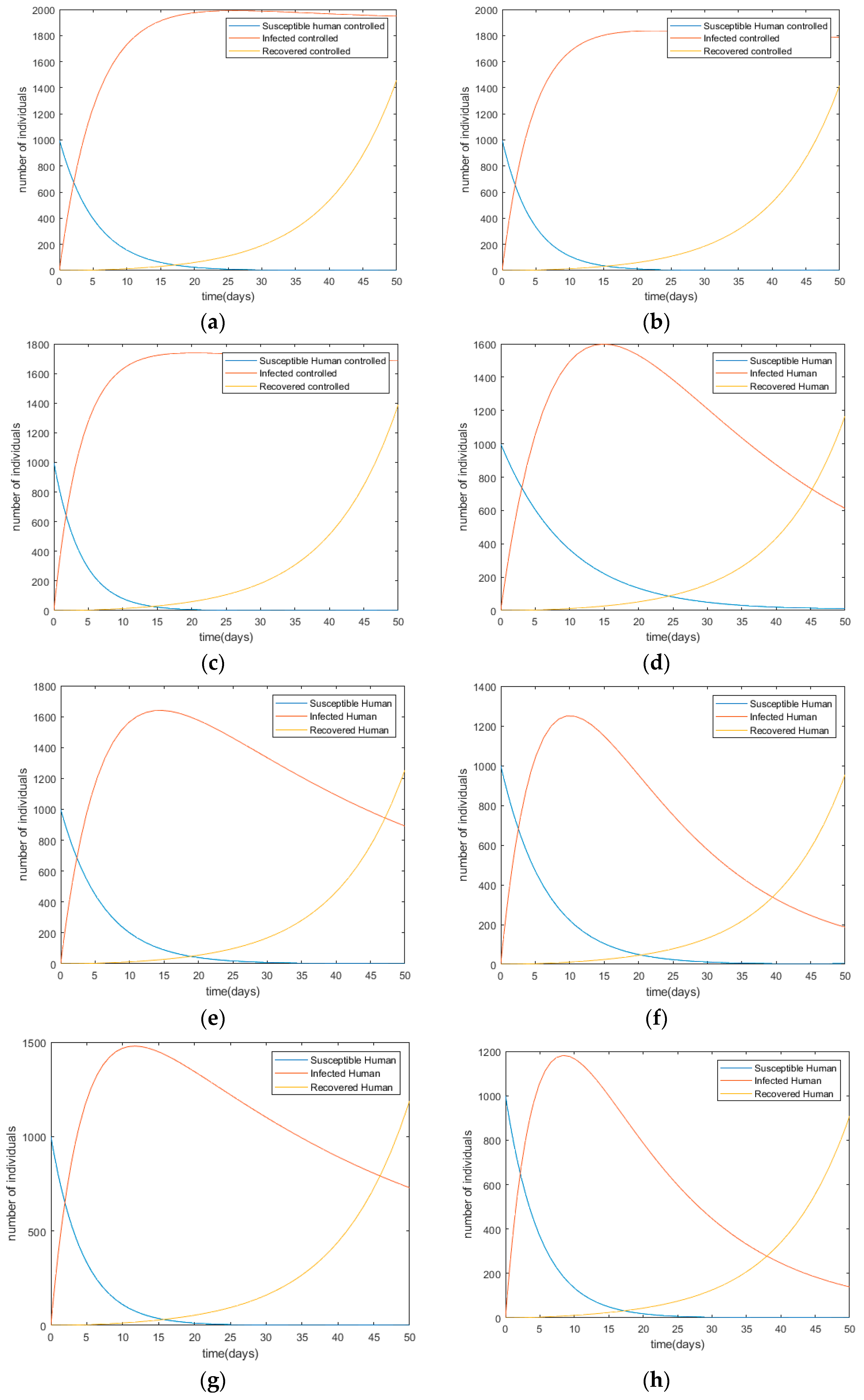
| Control Scenario | Relevant Figure | Cost ($) | Results |
|---|---|---|---|
| I | Figure 4a | 413,632 |
|
| II | Figure 4b | 381,605 |
|
| III | Figure 4c | 361,430 |
|
| IV | Figure 4d | 333,250 |
|
| V | Figure 4e | 340,836 |
|
| VI | Figure 4f | 261,131 |
|
| VII | Figure 4g | 307,556 |
|
| VIII | Figure 4h | 246,979 |
|
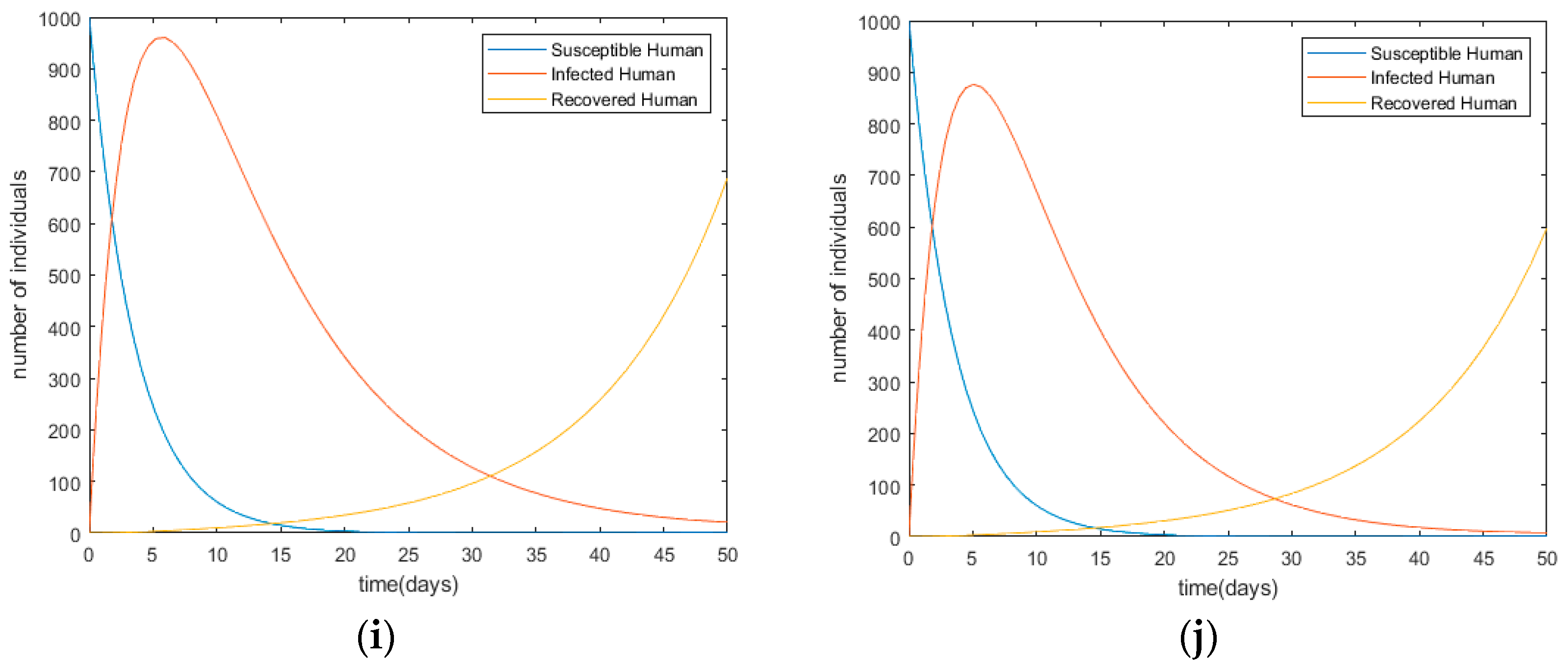
| IX | Figure 4i | 199,940 |
|
| X | Figure 4j | 183,691 |
|
© 2020 by the authors. Licensee MDPI, Basel, Switzerland. This article is an open access article distributed under the terms and conditions of the Creative Commons Attribution (CC BY) license (http://creativecommons.org/licenses/by/4.0/).
Share and Cite
Rahmadani, F.; Lee, H. Dynamic Model for the Epidemiology of Diarrhea and Simulation Considering Multiple Disease Carriers. Int. J. Environ. Res. Public Health 2020, 17, 5692. https://doi.org/10.3390/ijerph17165692
Rahmadani F, Lee H. Dynamic Model for the Epidemiology of Diarrhea and Simulation Considering Multiple Disease Carriers. International Journal of Environmental Research and Public Health. 2020; 17(16):5692. https://doi.org/10.3390/ijerph17165692
Chicago/Turabian StyleRahmadani, Firda, and Hyunsoo Lee. 2020. "Dynamic Model for the Epidemiology of Diarrhea and Simulation Considering Multiple Disease Carriers" International Journal of Environmental Research and Public Health 17, no. 16: 5692. https://doi.org/10.3390/ijerph17165692
APA StyleRahmadani, F., & Lee, H. (2020). Dynamic Model for the Epidemiology of Diarrhea and Simulation Considering Multiple Disease Carriers. International Journal of Environmental Research and Public Health, 17(16), 5692. https://doi.org/10.3390/ijerph17165692