Abstract
Currently, more and more remotely sensed data are being accumulated, and the spatial analysis methods for remotely sensed data, especially big data, are desiderating innovation. A deep convolutional network (CNN) model is proposed in this paper for exploiting the spatial influence feature in remotely sensed data. The method was applied in investigating the magnitude of the spatial influence of four factors—population, gross domestic product (GDP), terrain, land-use and land-cover (LULC)—on remotely sensed concentration over China. Satisfactory results were produced by the method. It demonstrates that the deep CNN model can be well applied in the field of spatial analysing remotely sensed big data. And the accuracy of the deep CNN is much higher than of geographically weighted regression (GWR) based on comparation. The results showed that population spatial density, GDP spatial density, terrain, and LULC could together determine the spatial distribution of annual concentrations with an overall spatial influencing magnitude of 97.85%. Population, GDP, terrain, and LULC have individual spatial influencing magnitudes of 47.12% and 36.13%, 50.07% and 40.91% on annual concentrations respectively. Terrain and LULC are the dominating spatial influencing factors, and only these two factors together may approximately determine the spatial pattern of annual concentration over China with a high spatial influencing magnitude of 96.65%.
1. Introduction
Remote sensing technology has developed rapidly since the 1960s [1], and an abundance of remote sensing data has been accumulated in this 50-year period. Although abundant remotely sensed data have been applied to many fields, such as ecology, environment, geography, etc., the spatial analysis method for remotely sensed lattice data desiderates innovation. A single spatial variable generally has autocorrelation [2] (i.e., spatial dependence [3,4]), and various spatial variables have correlation. Spatial autocorrelations can be analysed with local indicators of the spatial association (LISA) index [5] (e.g., local Moran I [6], local Geary c index [7]). The main objective of spatial analysis is to identify the natural relationships that exist between variables [8,9]. The mainstream classical spatial analysis models, e.g., spatial lag model [10,11], spatial error model [10,11], and Bayesian spatial regression model [12], can only evaluate the overall or average linear correlation feature over a whole study region, neglecting the details of local area. These methods ignore the consequences of spatial heterogeneity [13]. The majority of spatial analysing methods assume stationary space. However, assuming spatial convariance structure to be stationary is not so reasonable [14]. The spatial influencing relationship can better be explored when the analysis is local and more detailed results can be yielded [15]. The inclusion of a spatial heterogeneity resulting from differences in environmental conditions, socioeconomic dynamics, and other factors reinforces the need for more regionalized spatial analyses in exposure assessment and public health [16]. Although, the geographically weighted regression (GWR) [17] method considers local details; however, it can only describe a linear or simple non-linear spatial influencing relationship. In the era of big data, the need for developing advanced spatial analysis methods (e.g., machine learning methods) for remotely sensed data is urgent.
Previously, there are several studies that have applied machine learning methods to address the influencing factors on concentrations. Zheng et al. [18] used traditional artificial neural networks to model spatial correlation between Beijing’s air qualities and influencing factors, e.g., meteorology, traffic flow, human mobility. Yan et al. [19] predicted the daily average PM2.5 concentration in Nanjing, Beijing, and Sanya, combining meteorological and contaminant factors based on the Long Short-Term Memory (LSTM) model. Suleiman et al. [20] presented a machine learning model to predict the traffic-related and concentrations from various variables (e.g., traffic variables). Hsieh et al. [21] proposed a semi-supervised learning algorithm to optimize the monitoring locations of air quality in Beijing based on spatial correlation. Certainly, there are some studies which utilized typical methods to investigate the influence of satellite-based PM2.5. He et al. [22] used empirical orthogonal function (EOF) to analyse the relationship between remotely sensed and climate circulation transformation in East China. Hajiloo et al. [23] employed geographical weight regression (GWR) to investigate impact of meteorological and environmental parameters on PM2.5 concentrations in Tehran, Iran. Yang et al. [24] quantified the influence of natural and socioeconomic factors on pollution using the GeoDetector model [25,26].
This study proposed a spatial analysis method that exploits the spatial influencing feature of remotely sensed data based on the deep CNN. CNN is a mainstream deep learning method and can effectively extract the feature representations from a large number of images [27] and object detection [28]. Some researchers have applied deep CNN in remote sensing classification. Q. Zou et al. [29] and Zhao et al. [30] proposed a DBN method for high-solution satellite imagery classification. H. Liang and Q. Li, C. Tao et al., and F.P.S. Luus et al. [31], Nogueira et al. [32], Volpi et al. [33], Chen et al. [34], have employed deep CNN in hyperspectral imagery classification or feature extraction. Some researchers have also employed deep CNN in synthetic aperture radar (SAR) image classification, e.g., Du et al. [35] and Geng et al. [36]. To our knowledge, the research applying deep CNN into spatial influencing of remotely sensed lattice data is very rare. This study aimed to present a deep CNN model exploiting the magnitude of spatial influence of four factors—population, gross domestic product (GDP), terrain, and land-use and land-cover (LULC)—to remotely sense the annual mean concentration of over China. This model not only considers local spatial heterogeneity but also has super nonlinear fitting ability. Therefore, the presented model is rooted in a deep learning framework and may reduce uncertainty of the results obtained from a simplistic correlation analysis or simple regression model, therefore giving better information to decision makers of public health.
2. Materials and Methodology
2.1. Materials
The materials used in this research contain five types of data: remotely sensed concentration, population spatial distribution density, GDP spatial distribution density, terrain data, and LULC in China. The remotely sensed PM2.5 annual concentration dataset in 2010 was produced by the Atmospheric Physics Institute of Dalhousie University in Canada [37] with a resolution of . The population density data in this paper are cited in the Gridded Population of the World (GPW), data of the UN-Adjust Population Density-v4 [38], published by a data centre in NASA’s Earth Observing System Data and Information System (EOSDIS), with a resolution of 30′ × 30′. GDP spatial distribution density, terrain data, and LULC datasets were drawn from the Resources and Environmental Science Centre of the Chinese Academy of Sciences (http://www.resdc.cn). All above-mentioned data were projected by Albers Conic Equal Area with WGS-84 datum, and the resolution was unified to .
2.2. Methodology
The methodology in this paper consists of two modules: processing geospatial data and structuring the deep CNN model. The purpose of the former is to establish the dataset for the deep CNN model. The deep CNN model undertakes the mission of fitting the complex function of spatial correlation relationship.
2.2.1. Processing Geospatial Data
The deep CNN method is usually applied in image identification or classification, not directly transplanted into analysing geospatial data. In the geospatial issue, spatial correlation and geographical attribute need to be considered. Hence, geospatial data require technical processing to match the deep CNN model structure. The four influencing factors generate inputs. Each pixel location contains concentrations as output and four influencing factors. In view of spatial correlation, the pixel location and the surrounding locations should be considered. The deep CNN model has the ability of processing big data; therefore the order of spatial correlation can be amplified. In this paper, the order of spatial correlation adopts n-order shape, pixels (). Figure 1 shows an illustration of 5-order shape of the spatial correlation extent, including pixels. Subsequently, it can extract the corresponding four sets of influencing factor attribute data for a pixel location. Each dataset of influencing factors comprises the corresponding values of the surrounding pixels. In short, the annual concentration of a pixel location is affected by the four influencing factors of its own and the surrounding n-order spatial correlation extent, pixels. The mathematic form can be expressed as follows:
where is the annual concentration of the i-th pixel, , ,, represent the four influencing factor attribute values of the i-th pixel and its surrounding pixels, and represents the error. The spatial influencing function can be learned by the deep CNN model.
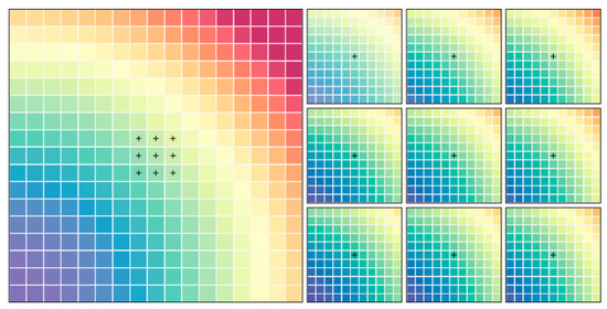
Figure 1.
Illustrating 5-order shape of the extent of spatial correlation.
2.2.2. A Developed Deep Convolutional Neural Network Model
CNN contains two categories of cells in the visual cortex, simple cells which exploit local features and complex cells which “pool” (e.g., maximizing, averaging) the outputs of simple cells within a neighbourhood. The structure of CNN model which has two special aspects of local connections and sharing weights is different from general deep learning models. A complete deep CNN stack three types of layers, convolutional layers, pooling layers, and full connected layers.
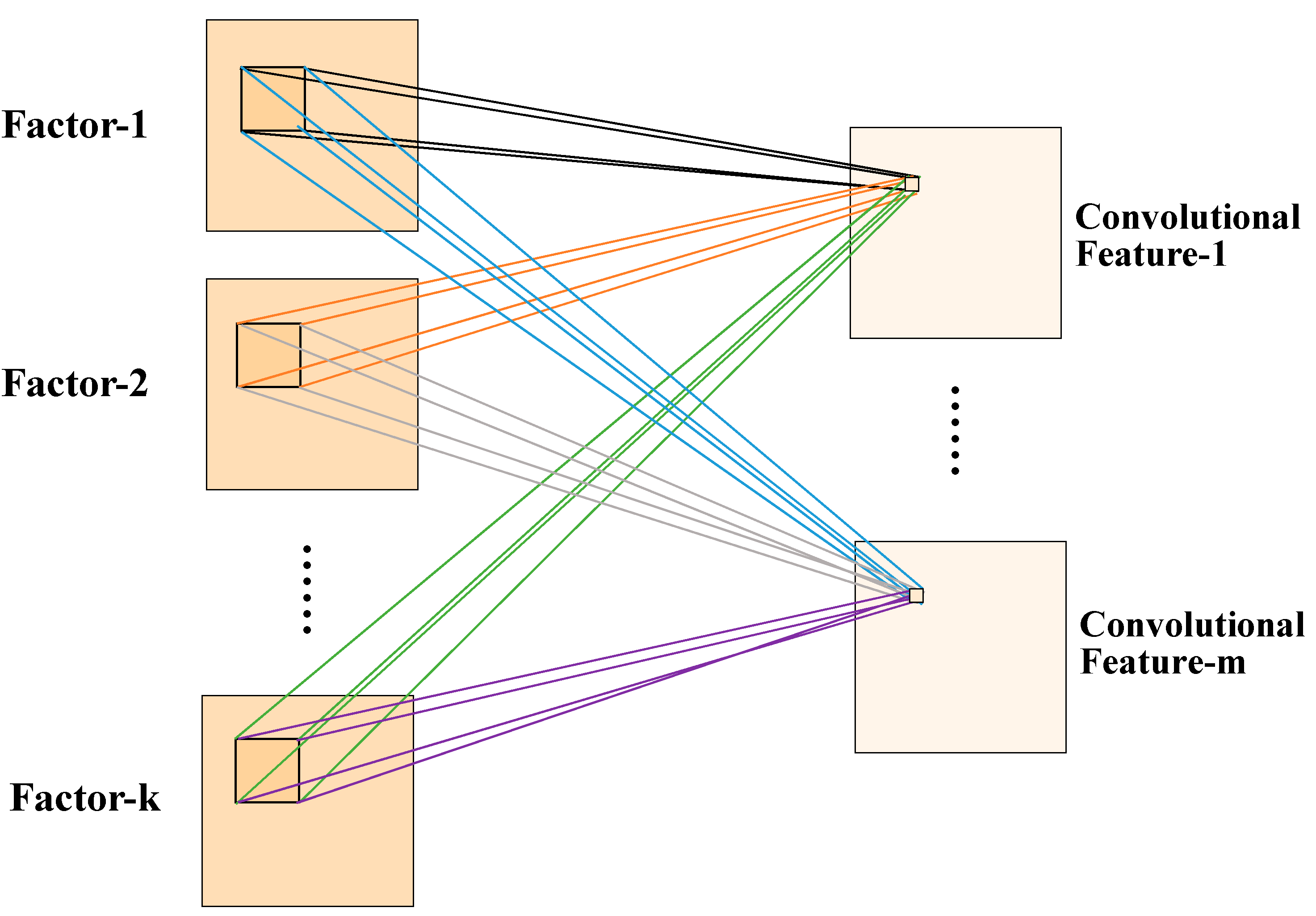
The commonly used CNNs are 2-Dimensional CNN and 3- Dimensional (3-D) CNN. Figure 2 shows a 3-D CNN illustration with m (m = 1, 2, …) filters and k (k = 1, 2, …) convolution kernels. The value of a neuron at position of the j-th convolutional feature in the i-th layer can be expressed as follows [34]:
where m indexes the convolutional feature in the th layer connected to the j-th convolutional feature, and and are the height and the width of the convolutional kernel. is the size of the spatial influencing factors, is the value of position connected to the m-th convolutional feature, and is the bias of the j-th convolutional feature in the i-th layer.
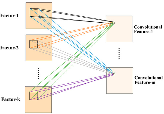
Figure 2.
The illustration of 3-D convolution with m (m = 1, 2, …) filters and k (k = 1, 2, …) convolution kernels, the weights are color-coded.
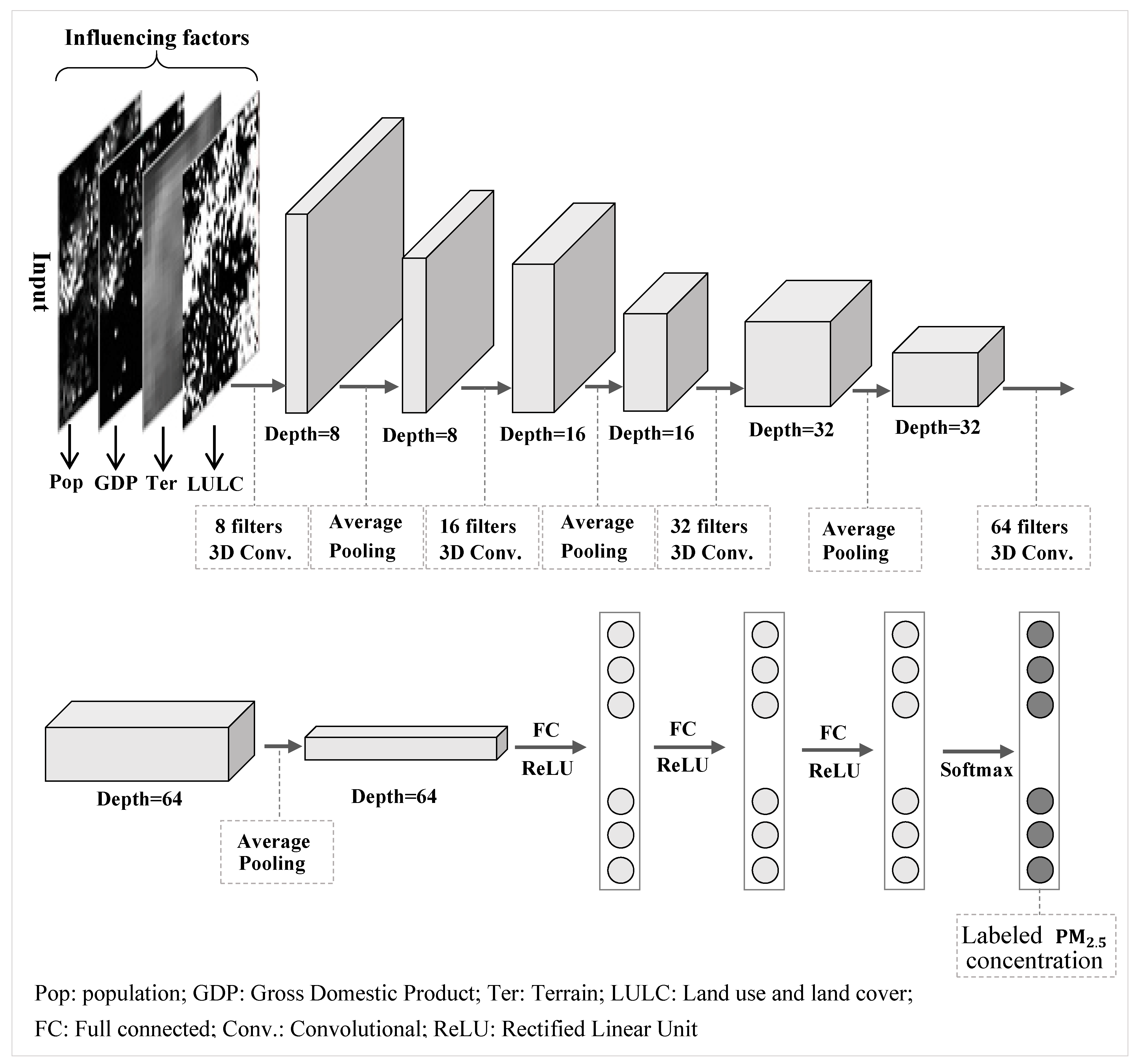
This paper designs a deep 3-D CNN model for exploiting spatial influencing feature of remotely sensed data. Figure 3 illustrates the presented deep CNN model architecture which contains including four convolutional layers, four polling layers, and three hidden layers. And the activation function for hidden layer adopted the Rectified Linear Unit (ReLU) function. The pooling mode employed average mode. The batch normalization was set in each layer except for the output layer. The dropout ratio and learning ratio were set as 25% and 1%, respectively. The dimension of the pre-processed input neural layer is , including four sets of influencing factors with the i-th pixel and its surrounding pixels. Table 1 lists the experimental results when the spatial correlation parameter n was assigned various values. It shows that the validation accuracy reaches the highest when the spatial correlation parameter, n, is taken 9, although the training accuracy is improved along with the increase of the parameter, n. Considering that the validation accuracy is better indicator representing the accuracy of a model. Hence, the spatial correlation parameter, n, is assigned with nine. Then the input layer contains 19 × 19 × 4 neurons with the four factors’ attribute value. The number of the output neuron is 11, labelled by annual concentration with 11 categories: <10 , , , , , , , , , , >100 .
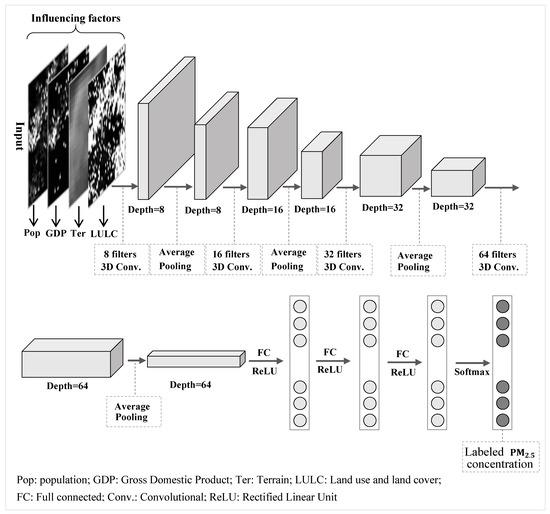
Figure 3.
Illustration of the presented deep CNN model architecture exploiting spatial influencing feature of remotely sensed concentration, including four convolutional layers, four polling layers, and three hidden layers, the first layer is input containing four influencing factors’ values on a pixel, the output layer with 11 neurons consisting of 11 categories of annual concentrations on the pixel location in the middle.

Table 1.
Experimental results of the training and validation accuracy of the deep 3-D CNN model when the spatial correlation parameter, n, is assigned various values
3. Results
The remotely sensed annual concentration and influencing factors possessed 96,337 pixels, among which, 86,903 pixels (accounting for the ratio of 90%) were used for deep learning, and the remaining 9434 pixels (accounting for 10%) were reserved for validation. Training accuracy is defined as the accuracy applied to the training data (i.e., 86,903 pixels), while validation accuracy is the accuracy for the remaining data (i.e., 9434 pixels), and estimated accuracy is the accuracy for the total data (i.e., 96,337 pixels). To investigate the integrated and respective spatial influence of the four various factors, we exploited the congregate magnitude of spatial influence from the four factors and the separate influencing magnitude from one or two factors.
3.1. Integrated Spatial Influencing Feature
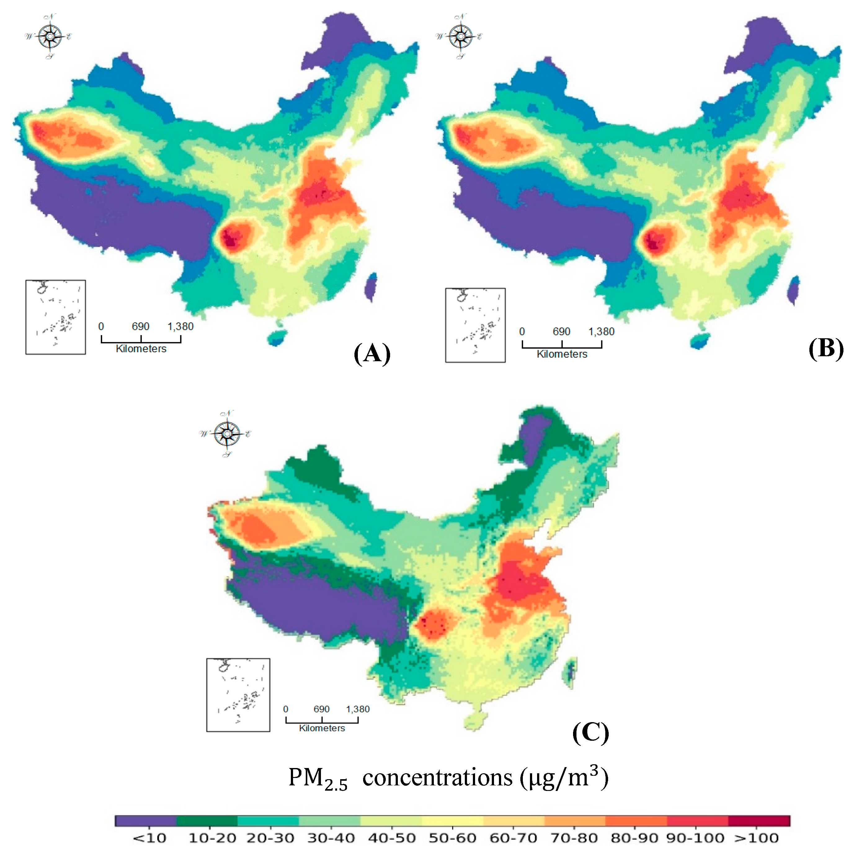
If the four impact factors were all fed into the input layer, after 1000 epochs of learning, the training accuracy of 86,903 pixels were 98.71%, and the validation accuracy of the remaining 9434 pixels reached 93.29%. Figure 4 illustrates the spatial distribution of the original and estimated annual concentration of the total 96,337 pixels using the trained deep learning model fed with the four influencing factors.

Figure 4.
Original (A), estimated spatial distribution of annual mean concentrations in 2010 (B) by the deep CNN model and (C) Geographic Weighted Regression (GWR) model, with the four influencing factors (population spatial density, GDP spatial density, terrain, and LULC) over China in 2010.
The estimated spatial distribution of annual concentration was nearly the same, except for very few pixel locations. It indicated that the four factors (population spatial density, GDP spatial density, terrain, and LULC) can almost determine the annual concentration. Furthermore, Table 2 listed the corresponding confusion matrix between the original and estimated annual concentration of the total 96,337 pixel locations by the four factors using the trained deep CNN model. The result showed that although there are some incorrect estimated pixel values which were close to the correct values, that is an obvious narrow diagonal band. The overall estimated accuracy is 97.85%. The estimated accuracy of the first category of annual concentration, <10 reaches a maximum of 99.38%. The minimum and the second minimum predicted accuracies are 90.81% and 95.48% respectively, occurring on the eighth and eleventh category of and . The estimated accuracy can be regarded as the spatial influencing magnitude of the influencing factors on annual concentration. A high estimated accuracy reflects directly a high spatial influencing feature. The results show that there is a strong correlation between annual concentration and the four factors. Especially while the trained deep CNN evaluated the total 96,337 pixels, the overall estimated accuracy has reached up to 97.85%, indicating the spatial influencing magnitude of the four factors on annual concentration.
Table 2.
The confusion matrix of the original vs. estimated annual concentrations by the deep CNN model fed by the four influencing factor data: population, GDP, terrain, and LULC.
3.2. Single Spatial Influencing Feature
The spatial influencing magnitude of the single factor can be measured by the deep CNN model proposed in this paper. We have implemented other deep CNNs whose input layer contains neurons with a single factor attribute value; the other parameters are the same as above. After 1000 epochs of learning, the training accuracy and validation accuracy of population spatial density and GDP spatial density were 47.12% and 36.13%, 50.07% and 40.91%. Furthermore, the results show that annual concentration has strong spatial correlation with terrain or LULC, as the validation accuracies of terrain and LULC were up to 83.17% and 72.37%. The result showed that although the overall estimated accuracies of population and GDP over China were relatively low, the two factors could have determined the severe polluted region. Furthermore, the result indicated that terrain and LULC are the main spatial influencing factors on annual concentration over China.
In addition, we also have implemented the deep CNN with an input layer containing neurons describing terrain and LULC. The learning result shows that the training accuracy and validation accuracy of the two factors, terrain and LULC, were up to 90.69% and 87.95%. Table 3 listed the corresponding confusion matrix between the original and estimated annual concentration produced by the trained deep CNN fed by terrain and LULC data on the total 96,337 pixel locations. Except for the eleventh category (>100 ) of annual concentration, the other ten categories’ estimated accuracies are more than 91%. Furthermore, the overall estimated precision can reach up to 96.65%.
Table 3.
The confusion matrix of the original vs. estimated annual concentrations by the deep CNN model fed by the two influencing factor data, terrain and LULC.
3.3. Comparation with the GWR Prediction
To verify the advantage of the deep CNN model presented in this paper, we conducted the GWR in the same dataset. Figure 4C is the estimated spatial distribution of annual concentrations over China in 2010 by the GWR model. It can be seen that the GWR estimated results have obvious bias comparing with the origin data (Figure 4). Furthermore, the lowest and highest concentrations were particularly misestimated by the GWR model. And the overall estimated accuracy was 72.81% which is more less than the estimated accuracy of the deep CNN model, 97.85%. Comparing the Figure 4B,C, it indicated that although the overall spatial structure estimated by the GWR is generally similar with the origin spatial structure of annual concentrations, there were some deviations in detail. The cause of the difference of the two models could be that, the deep CNN model has super strong non-linear fitting ability which can train very complicated non-linear function, however, the GWR is still a linear regression model which cannot catch complicated non-linear variation effects. Inaccurate correlativity between concentration and other influencing factors could lead to biased public policies. Scientific public policy-making need more fine and accurate analysing evidences.
4. Discussion
This study proposed a deep CNN model to exploit spatial influencing magnitude for the annual mean concentration of remotely sensed over China. In consideration of the influencing mechanism and the availability of the dataset, this study investigated the spatial influence of the four factors (population, GDP, terrain, and LULC) on the annual concentration of over China. The influencing factors of pollution are known to include natural and anthropogenic activities [39]. Among the four factors selected for this paper, terrain represented natural elements, population and GDP reflected anthropogenic activities, and LULC could be regarded as a mixture of natural and anthropogenic activities. The presented deep CNN method fully considered the local spatial heterogeneity, and a wider spatial correlated scope could be considered by more than one-order shape extent, which benefited from the strong ability of the deep CNN to process big data.
This paper bridged the gap between spatial analysis and deep CNN technology with the idea of reprocessing or reorganizing remotely sensed data for deep CNN input. The deep CNN method was commonly used to extract the feature representations from a mass of labelled images [27,28]. As aforesaid, few researchers applied the deep CNN model when analysing spatial influence of multiple variables. From a different view, combining a geospatial reprocess, this study designed a 3D deep CNN structure in which the input and output neurons were influencing factors and concentration, respectively. The strong non-linear function fitting ability of a deep CNN model could then detect complicated non-linear spatial influencing effect, and the deep CNN model might consider local spatial heterogeneity. From the results, the developed deep CNN model can fully consider spatial relationship and can calculate on each pixel location. Hence, the results can effectively describe the spatial influencing feature on every pixel location. Although the GWR method can also investigate the local correlation on each pixel location, only a linear or simple non-linear regression can be implemented, and the capability of processing big data is not very strong. From the above, the deep CNN model can not only process big data well but can also fit or learn very complicated correlativity.
This paper demonstrated that the deep CNN technology could be applied in exploiting the spatial influence feature of geospatial or remotely sensed data, and its advantages could be fully performed. The spatial influencing magnitude of the four factors on the annual concentration of was investigated employing the presented deep CNN model. This model was not only used in exploring spatial influence of remotely sensed concentration, but also in other fields, such as detecting risk factors of some kind of epidemic based on remotely sensed data. Through the model, the risk level of risk factors in public health could be quantificationally assessed. In other words, the developed deep CNN model has the potential to expand the field of spatial analysis of remotely sensed lattice data. Despite all this, this research has some limitations. Firstly, the spatial dependent variable, annual concentration, is classified into 11 categories, not as a continuous variable. Secondly, the deep CNN model can learn a very complicated function structure, but the mathematical mechanism is currently not clear, namely mysterious “black boxes” [40], and it is difficult to explain in a geographical process.
5. Conclusions
Population spatial density, GDP spatial density, terrain, and LULC can almost determine the spatial pattern of annual concentration with an overall estimated precision of 97.85% over China. Furthermore, terrain and LULC are the main spatial influencing factors on annual concentration among the four factors. And the overall spatial influencing magnitude of the two factors, terrain and LULC, reached up to 96.65%, nearly equal to all four factors’ spatial influencing magnitude on annual concentration.
Author Contributions
J.L. and M.J. conceived and designed the experiments; J.L. performed the experiments; M.J. and H.L. analyzed the data; J.L. wrote the paper.
Funding
National Natural Science Youth Foundation of China (61801279).
Acknowledgments
The authors are grateful to all the peer reviewers for this paper, as well as to Aron van Donkelaar’s team at Dalhousie University in Canada, who produced the annual mean PM2.5 concentration data used in this paper.
Conflicts of Interest
The authors declare no conflict of interest.
References
- Geng, J.; Wang, H.; Fan, J.; Ma, X. Deep supervised and contractive neural network for SAR image classification. IEEE Trans. Geosci. Remote Sens. 2017, 55, 2442–2459. [Google Scholar] [CrossRef]
- Van, D.A.; Martin, R.V.; Brauer, M.; Hsu, N.C.; Kahn, R.A.; Levy, R.C.; Lyapustin, A.; Sayer, A.M.; Winker, D.M. Global estimates of fine particulate matter using a combined geophysical-statistical method with information from satellites, models, and monitors. Environ. Sci. Technol. 2016, 50, 3762–3772. [Google Scholar]
- Center for International Earth Science Information Network—CIESIN—Columbia University. Gridded Population of the World, Version 4 (gpwv4): Population Density Adjusted to Match 2015 Revision UN WPP Country Totals; NASA Socioeconomic Data and Applications Center (SEDAC): Palisades, NY, USA, 2016. [Google Scholar]
- Lin, G.; Fu, J.; Jiang, D.; Hu, W.; Dong, D.; Huang, Y.; Zhao, M. Spatio-temporal variation of PM2.5 concentrations and their relationship with geographic and socioeconomic factors in China. Int. J. Environ. Res. Public Health 2013, 11, 173–186. [Google Scholar] [CrossRef] [PubMed]
- Alain, G.; Bengio, Y. Understanding intermediate layers using linear classifier probes. arXiv, 2016; arXiv:1610.01644. [Google Scholar]
- Ward, S.; Bond, P. The Earth Observation Handbook; European Space Agency: Paris, France, 2008; Volume 1315. [Google Scholar]
- Tobler, W.R. A computer movie simulating urban growth in the Detroit Region. Econ. Geogr. 1970, 46, 234–240. [Google Scholar] [CrossRef]
- Cressie, N. Statistics for Spatial Data; Wiley: Hoboken, NJ, USA, 1993; pp. 321–323. [Google Scholar]
- Haining, R. Spatial Data Analysis; Cambridge University Press: Cambridge, UK, 2003. [Google Scholar]
- Anselin, L. Local indicators of spatial association—Lisa. Geogr. Anal. 1995, 27, 93–115. [Google Scholar] [CrossRef]
- Boots, B. Local measures of spatial association. Écoscience 2002, 9, 168–176. [Google Scholar] [CrossRef]
- Getis, A.; Ord, J.K. The analysis of spatial association by use of distance statistics. Geogr. Anal. 1992, 24, 189–206. [Google Scholar] [CrossRef]
- Brunsdon, C.; Fotheringham, A.S.; Charlton, M.E. Geographically weighted regression: A method for exploring spatial nonstationarity. Geogr. Anal. 1996, 28, 281–298. [Google Scholar] [CrossRef]
- Fotheringham, A.S.; Charlton, M.E.; Brunsdon, C. Geographically weighted regression: A natural evolution of the expansion method for spatial data analysis. Environ. Plan. A 1998, 30, 1905–1927. [Google Scholar] [CrossRef]
- Anselin, L. Spatial econometric: Methods and models. J. Am. Stat. Assoc. 1990, 85, 160. [Google Scholar]
- Anselin, L.; Bera, A.K.; Florax, R.; Yoon, M.J. Simple diagnostic tests for spatial dependence. Reg. Sci. Urban Econ. 1996, 26, 77–104. [Google Scholar] [CrossRef]
- Gschlößl, S. Hierarchical Bayesian Spatial Regression Models with Applications to Non-Life Insurance. Ph.D. Thesis, Technische Universität München, München, Germany, 2006. [Google Scholar]
- Feuillet, T.; Commenges, H.; Menai, M.; Salze, P.; Perchoux, C.; Reuillon, R.; Kesse-Guyot, E.; Enaux, C.; Nazare, J.-A.; Hercberg, S. A massive geographically weighted regression model of walking-environment relationships. J. Transp. Geogr. 2018, 68, 118–129. [Google Scholar] [CrossRef]
- Sampson, P.D.; Guttorp, P. Nonparametric estimation of nonstationary spatial covariance structure. J. Am. Stat. Assoc. 1992, 87, 108–119. [Google Scholar] [CrossRef]
- Duarte-Cunha, M.; Almeida, A.S.d.; Cunha, G.M.d.; Souza-Santos, R. Geographic weighted regression: Applicability to epidemiological studies of leprosy. Rev. Soc. Bras. Med. Trop. 2016, 49, 74–82. [Google Scholar] [CrossRef] [PubMed]
- Fischer, E.; Pahan, D.; Chowdhury, S.; Richardus, J. The spatial distribution of leprosy cases during 15 years of a leprosy control program in Bangladesh: An observational study. BMC Infect. Dis. 2008, 8, 126. [Google Scholar] [CrossRef]
- Lesage, J.P. A Family of Geographically Weighted Regression Models; Springer: Berlin/Heidelberg, Germany, 2004; pp. 241–264. [Google Scholar]
- Zheng, Y.; Liu, F.; Hsieh, H.P. U-air: When urban air quality inference meets big data. In Proceedings of the ACM SIGKDD International Conference on Knowledge Discovery and Data Mining, Chicago, IL, USA, 11–14 August 2013; pp. 1436–1444. [Google Scholar]
- Yan, L.; Zhou, M.; Wu, Y.; Yan, L. Long short term memory model for analysis and forecast of PM2.5. In Proceedings of the International Conference on Cloud Computing and Security, Haikou, China, 8–10 June 2018; Springer: Berlin/Heidelberg, Germany, 2004; pp. 623–634. [Google Scholar]
- Suleiman, A.; Tight, M.; Quinn, A. Applying machine learning methods in managing urban concentrations of traffic-related particulate matter (PM10 and PM2.5). Atmos. Pollut. Res. 2019, 10, 134–144. [Google Scholar] [CrossRef]
- Hsieh, H.P.; Lin, S.D.; Zheng, Y. Inferring air quality for station location recommendation based on urban big data. In Proceedings of the 21th ACM SIGKDD International Conference on Knowledge Discovery and Data Mining, Sydney, Australia, 10–13 August 2015; pp. 437–446. [Google Scholar]
- He, Q.; Geng, F.; Li, C. Long-term variation of satellite-based PM2.5 and influence factors over east China. Sci. Rep. 2018, 8. [Google Scholar] [CrossRef]
- Hajiloo, F.; Hamzeh, S.; Gheysari, M. Impact assessment of meteorological and environmental parameters on PM2.5 concentrations using remote sensing data and GWR analysis (case study of Tehran). Environ. Sci. Pollut. Res. 2018, 1–15. [Google Scholar]
- Yang, D.; Wang, X.; Xu, J.; Xu, C.; Lu, D.; Ye, C.; Wang, Z.; Bai, L. Quantifying the influence of natural and socioeconomic factors and their interactive impact on PM2.5 pollution in China. Environ. Pollut. 2018, 241, 475–483. [Google Scholar] [CrossRef]
- Wang, J.F.; Li, X.H.; Christakos, G.; Liao, Y.L.; Zhang, T.; Gu, X.; Zheng, X.Y. Geographical detectors-based health risk assessment and its application in the neural tube defects study of the Heshun Region, China. Int. J. Geogr. Inf. Sci. 2010, 24, 107–127. [Google Scholar] [CrossRef]
- Wang, J.F.; Zhang, T.L.; Fu, B.J. A measure of spatial stratified heterogeneity. Ecol. Indic. 2016, 67, 250–256. [Google Scholar] [CrossRef]
- Krizhevsky, A.; Sutskever, I.; Hinton, G.E. Imagenet classification with deep convolutional neural networks. In Proceedings of the International Conference on Neural Information Processing Systems, Doha, Qatar, 12–15 November 2012; pp. 1097–1105. [Google Scholar]
- Girshick, R.; Donahue, J.; Darrell, T.; Malik, J. Region-based convolutional networks for accurate object detection and segmentation. IEEE Trans. Pattern Anal. Mach. Intell. 2016, 38, 142–158. [Google Scholar] [CrossRef] [PubMed]
- Zou, Q.; Ni, L.; Zhang, T.; Wang, Q. Deep learning based feature selection for remote sensing scene classification. IEEE Geosci. Remote Sens. Lett. 2015, 12, 2321–2325. [Google Scholar] [CrossRef]
- Zhao, Z.; Jiao, L.; Zhao, J.; Gu, J.; Zhao, J. Discriminant deep belief network for high-resolution SAR image classification. Pattern Recognit. 2017, 61, 686–701. [Google Scholar] [CrossRef]
- Liang, H.; Li, Q. Hyperspectral imagery classification using sparse representations of convolutional neural network features. Remote Sens. 2016, 8, 99. [Google Scholar] [CrossRef]
- Nogueira, K.; Penatti, O.A.B.; Santos, J.A.D. Towards better exploiting convolutional neural networks for remote sensing scene classification. Pattern Recognit. 2017, 61, 539–556. [Google Scholar] [CrossRef]
- Volpi, M.; Tuia, D. Dense semantic labeling of subdecimeter resolution images with convolutional neural networks. IEEE Trans. Geosci. Remote Sens. 2016, PP, 1–13. [Google Scholar] [CrossRef]
- Chen, Y.; Jiang, H.; Li, C.; Jia, X.; Ghamisi, P. Deep feature extraction and classification of hyperspectral images based on convolutional neural networks. IEEE Trans. Geosci. Remote Sens. 2016, 54, 6232–6251. [Google Scholar] [CrossRef]
- Du, K.; Deng, Y.; Wang, R.; Zhao, T.; Li, N. Sar atr based on displacement- and rotation-insensitive CNN. Remote Sens. Lett. 2016, 7, 895–904. [Google Scholar] [CrossRef]

© 2019 by the author. Licensee MDPI, Basel, Switzerland. This article is an open access article distributed under the terms and conditions of the Creative Commons Attribution (CC BY) license (http://creativecommons.org/licenses/by/4.0/).