Article

Utilization of the Maryland Environmental Justice Screening Tool: A Bladensburg, Maryland Case Study

1
Public Health Science Program, University of Maryland, 255 Campus Drive, College Park, MD 20740, USA
2
Environmental Science and Technology Department, University of Maryland, 1451 Animal Science Bldg, College Park, MD 20742-2315, USA
3
Department of Psychology, Swarthmore College, 500 College Ave, Swarthmore, PA 19081, USA
4
Maryland Institute for Applied Environmental Health, University of Maryland, 255 Valley Drive, College Park, MD 20742, USA
*
Author to whom correspondence should be addressed.
Int. J. Environ. Res. Public Health 2019, 16(3), 348; https://doi.org/10.3390/ijerph16030348
Submission received: 21 November 2018 / Revised: 21 January 2019 / Accepted: 22 January 2019 / Published: 26 January 2019

Abstract

:
Maryland residents’ knowledge of environmental hazards and their health effects is limited, partly due to the absence of tools to map and visualize distribution of risk factors across sociodemographic groups. This study discusses the development of the Maryland EJSCREEN (MD EJSCREEN) tool by the National Center for Smart Growth in partnership with faculty at the University of Maryland School of Public Health. The tool assesses environmental justice risks similarly to the U.S. Environmental Protection Agency’s (USEPA) EJSCREEN tool and California’s tool, CalEnviroScreen 3.0. We discuss the architecture and functionality of the tool, indicators of importance, and how it compares to USEPA’s EJSCREEN and CalEnviroScreen. We demonstrate the use of MD EJSCREEN through a case study on Bladensburg, Maryland, a town in Prince George’s County (PG) with several environmental justice concerns including air pollution from traffic and a concrete plant. Comparison reveals that environmental and demographic indicators in MD EJSCREEN most closely resemble those in EPA EJSCREEN, while the scoring is most similar to CalEnviroScreen. Case study results show that Bladensburg has a Prince George’s environmental justice score of 0.99, and that National Air Toxics Assessment (NATA) air toxics cancer risk is concentrated in communities of color.

1. Introduction

Environmental justice research since the 1970s has illustrated siting disparities of environmental hazards and locally unwanted land uses (LULUs) in communities of color [1,2,3,4,5]. Specifically, these neighborhoods are disproportionately burdened by noxious facilities that threaten the social, environmental, and physical health of local residents [5,6,7,8,9]. There are a number of environmental stressors that affect the physical and social well-being of a population such as: (1) proximity to hazardous waste sites, (2) exposure to air and water pollution, (3) residential crowding, (4) high levels of ambient noise, (5) the work environment, and (6) quality of local schools [8,9,10,11]. These harmful exposures have been examined using Geographic Information System (GIS) and Public Participatory Geographic Information System (PPGIS) mapping tools. The use of GIS and PPGIS in public health research has produced a wealth of information that can be used to improve the quality of life in overburdened neighborhoods.
GIS is a mapping tool which can be used to visualize the spatial distribution of pathogenic and salutogenic elements in the environment [12]. GIS is central to studying environmental justice because it illustrates how social, economic, and racial stratification have reinforced the disproportionate burden of environmental health hazards on marginalized communities. Studies using this technology have found that low income and communities of color are more likely to be located near pollution sources [13,14,15,16]. GIS has also been utilized in studies of traffic-related air pollution (TRAP) and water pollution in overburdened communities [17,18,19,20]. The presence of such environmental hazards, as well as walkable streets and parks, food quality around schools, and supermarket accessibility have all served as indicators of community wellness [21,22,23].
These findings have been mirrored by PPGIS studies on environmental hazards in vulnerable communities [13,24]. Studies utilizing this visualization approach have stressed the importance of incorporating the lived experiences of community members in environmental health research [25,26,27]. PPGIS integrates local and government knowledge on pollution sources to build community capacity and empower citizens to take active roles in environmental justice discussions [27,28,29]. PPGIS has been used to investigate the presence of urban blue spaces and aquatic environments, urban green spaces, community revitalization efforts, national forests, and land use [26,30,31,32,33,34].
GIS and PPGIS serve as crucial components of the California Communities Environmental Health Screening tool (i.e., CalEnviroScreen), which was created by the Office of Environmental Health Hazard Assessment (OEHHA) and California Environmental Protection Agency (CalEPA) in 2013. CalEnviroScreen uses mapping and screening techniques at the census-tract level to identify vulnerable communities that are disproportionately burdened by environmental hazards in the state of California [10]. The tool assigns cumulative impact scores, also referred to as CalEnviroScreen Scores, to each census tract as a measure of environmental inequality [8,35].
Another tool which applies a similar methodology on a national level is known as EJSCREEN (hereby referred to as EPA EJSCREEN for clarity), released in 2015 by the United States Environmental Protection Agency (US EPA). The tool’s purpose is to consolidate demographic and environmental health data from a multitude of publicly available sources into maps and reports [36,37]. This enables researchers and the general public to compare the state of environmental justice in marginalized communities to state, regional, and national averages [36,37].
CalEnviroScreen and EPA EJSCREEN exist to examine the environmental burdens within an area of interest. A team from the National Center for Smart Growth and School of Public Health helped to develop a preliminary version of a screening tool for the state of Maryland known as MD EJSCREEN. MD EJSCREEN was built upon the framework of the aforementioned tools using feedback gathered from stakeholders and community members in Prince George’s County. In attempts to further develop another mapping tool, MD EJSCREEN was created to focus on identifying disadvantaged communities. Although EPA EJSCREEN is able to map the entire US, it is unable to address all issues relevant at the local level due to the broad scope of the tool. MD EJSCREEN incorporates additional indicators that are more specific to Maryland such as: asthma emergency discharges and watershed failure. In addition, EPA EJSCREEN differs in its scale of analysis, and its ability to compute a score of environmental justice like MD EJSCREEN and CalEnviroScreen, making the development of a tool specific to Maryland all the more necessary.
This paper will discuss the development of MD EJSCREEN, community feedback received during a series of demonstration workshops, the architecture of the tool, how it compares to other environmental justice visualization tools, scoring methodology, and its application for Bladensburg, Maryland, a town in Prince George’s County.

2. Materials and Methods

Through a series of demonstration workshops, feedback was gathered from groups of stakeholders including Prince George’s County residents in order to develop, improve, and determine any and all environmental, population, and health indicators that would be included in MD EJSCREEN. The majority of the stakeholders included Prince George’s County Environmental Action Council (EAC) members, Port Towns residents, the environmental justice legislative team (EJLT), and the statewide Commission on Environmental Justice and Sustainable Communities. In order to obtain feedback on the indicators that were deemed necessary and acceptable for MD EJSCREEN, posters containing lists of different indicators were displayed at the stakeholder meetings. Surveys were also distributed to all stakeholders to gather feedback regarding the decidedly necessary and acceptable indicators that were to be highlighted in MD EJSCREEN.
The first stakeholder meeting occurred with the Prince George’s County EAC, an organization that presents feedback on environmental concerns to the Prince George’s County Department of the Environment. The feedback concerning each indicator was documented on flashcards and shared with the EJSCREEN development team. This information was used to build MD EJSCREEN.
Posters highlighting the relevance of each specified indicator were displayed at other stakeholder meetings. For instance, posters were displayed on site at Bladensburg Waterfront Park, and attendees were instructed to rank the importance of each indicator in the community. Four stickers were used to capture feedback from the stakeholders on listed indicators: (1) green, (2) blue, (3) yellow, and (4) red symbolizing very important, important, somewhat important, and not important, respectively. Unfortunately, the significance of each colored sticker became inconsistent for each individual stakeholder. To account for this issue, we removed the important/not important value from each sticker, and instead counted the physical number of stickers placed on each indicator to properly reflect the significance of each indicator. In the development of MD EJSCREEN, community members advocated for the inclusion of seven indicators to highlight the aspects of economic, environmental, and exposure factors that can significantly alter community health. The seven indicators were: (1) asthma emergency room discharges; (2) percent non-White; (3) proximity to treatment, storage, and disposal facilities (TSDFs); (4) myocardial infarction discharges; (5) low birth weight infants; (6) particulate matter (PM2.5); and (7) pathogenic infrastructure. Of these indicators, only pathogenic infrastructure was not mapped due to lack of sufficient data.
Additional feedback was obtained through surveys that asked community members to prioritize indicators taken from EPA EJSCREEN, CalEnviroScreen, and new indicators suggested by community members. A Likert scale was used to rank indicators by importance, in which a score of 1 indicated that said indicator was of low priority and a score of 5 indicated that it was of high priority. These surveys were distributed to several stakeholder groups including, the Association of Baltimore Area Grantmakers (ABAG), the Commission on Environmental Justice and Sustainable Communities, the Prince George’s County EAC, and the EJLT.

3. Results

MD EJSCREEN allows users to create interactive maps of demographic and environmental health within four primary categories: (1) Pollution Burden: Exposure; (2) Pollution Burden: Effect; (3) Population Characteristics: Sensitive Populations; and (4) Population Characteristics: Socioeconomic Factors. Each of these categories (Figure 1) contain a number of environmental justice indicators which are defined in Table 1.

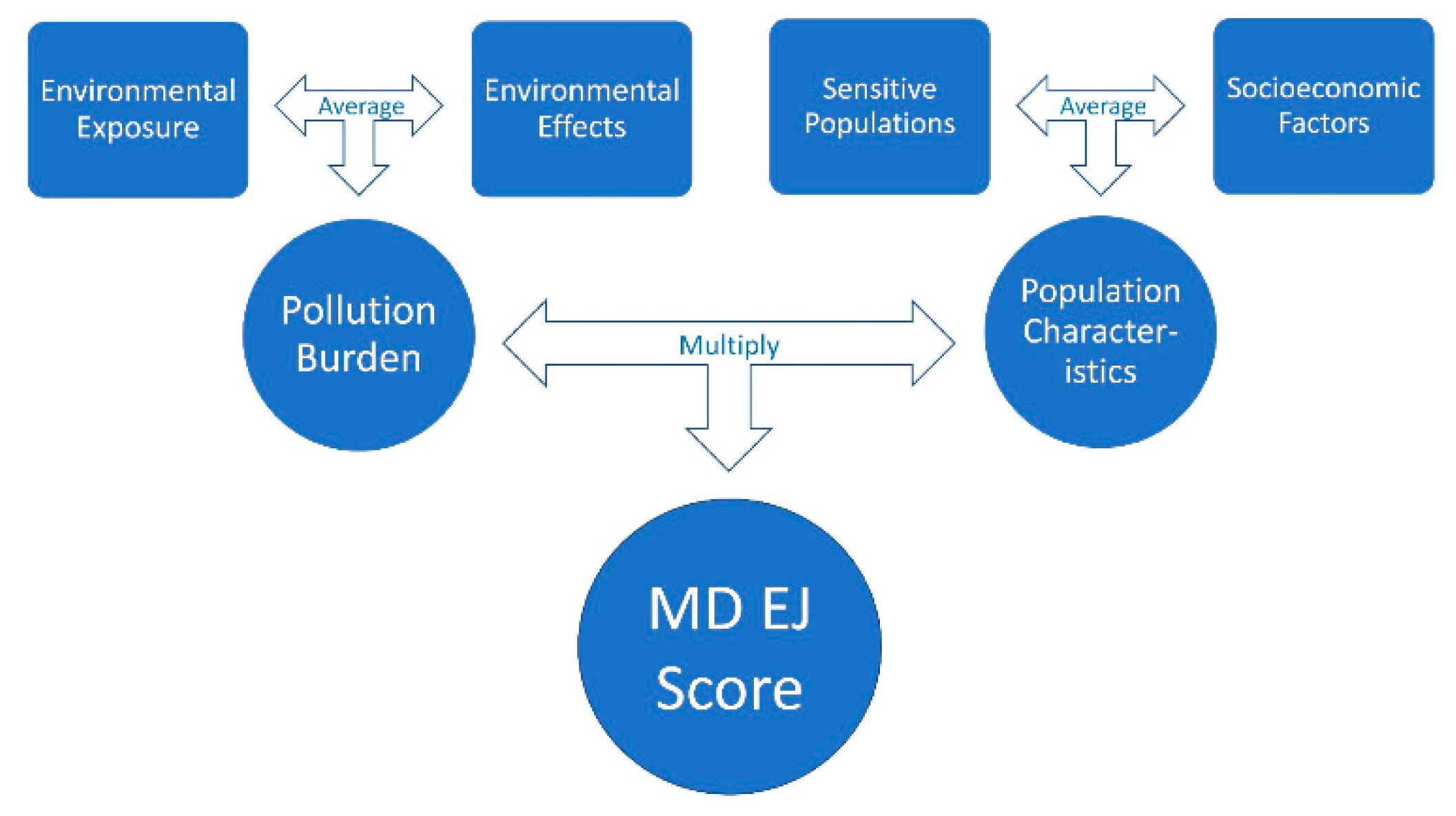
3.1. Scoring Process

MD EJSCREEN illustrates the extent of environmental injustice in an area by assigning an EJ Score to each census tract. To calculate the MD EJ score, the tool applies the methodology used by CalEnviroScreen [8]. A MD EJ score is calculated by first converting the raw indicator scores within each of the four categories: (1) Pollution Burden: Exposure; (2) Pollution Burden: Effect; (3) Population Characteristics: Sensitive Populations; and (4) Population Characteristics: Socioeconomic Factors into percentiles. The raw indicator scores are ranked from lowest to highest at the census-tract level, and then assigned percentile values from 0 to 1 based on how the indicator scores compare to other census tracts in the state. MD EJSCREEN also produces a PG EJ score, which applies the same methodology, but assigns percentile values from 0 to 1 based on how the indicator scores compare to other census tracts in Prince George’s County.
These values are averaged to create two scores per census tract: (1) the Population Characteristics score, and (2) the Pollution Burden score. The Population Characteristics score is the average of all indicators in the Sensitive Populations and Socioeconomic Factors categories. The Pollution Burden score is the average of all indicators in the Environmental Effects and Exposures categories. In this calculation; however, the Environmental Effects component is half-weighted. This means that the Environmental Effects category has a weight equal to 1/3, while the Environmental Exposure category has a weight equal to 2/3. This is done because Environmental Effects make a smaller contribution to Pollution Burden than Environmental Exposures.
To calculate the EJ scores, the Population Characteristics score is multiplied by the Pollution Burden score [38]. This score is reported as a percentile value 0 to 1 based on how it compares to other census tracts. An EJ score illustrates the magnitude of environmental justice concern in an area; thus, areas with high concentrations of low-income and/or non-White populations and high exposures to environmental hazards will have scores closer to 1.

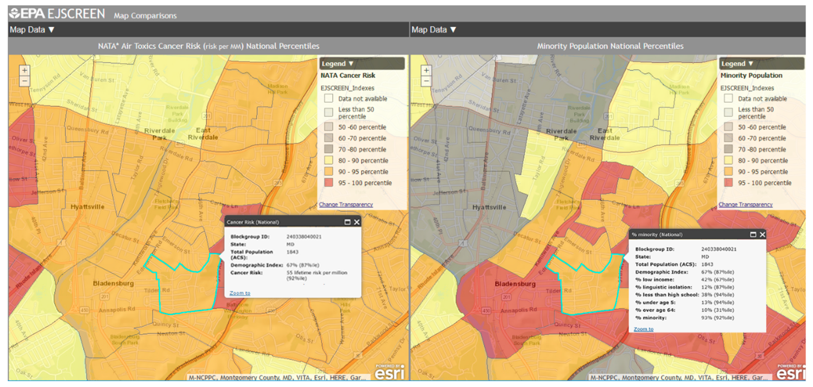
3.2. Comparison of MD EJSCREEN to CalEnviroScreen and EPA EJSCREEN

While MD EJCREEN, CalEnviroScreen, and EPA EJSCREEN all aid users in increasing environmental awareness, there are a number of differences in the usability, functionality, and type of information used in each tool. For instance, EPA EJSCREEN contributes useful demographic and environmental indicator data; however, the broad national scope of the tool limits the specificity and relevance of a given block group or census tract. CalEnviroScreen on the other hand, provides specific population characteristics and pollution burden data for the state for California and more importantly, has proved to be an apt model for MD EJSCREEN. However, CalEnviroScreen is missing pertinent information on Maryland specific indicators such as lead paint prevalence.
NATA respiratory hazard index, and Proximity to risk management plan (RMP) sites. A comparison of the usability and functionality of each tool is provided in Table 3.
In terms of specific indicators, the tools have a number of similarities and differences. Table 1 displays a comparison of indicators included in CalEnviroScreen, EPA EJSCREEN, and MD EJSCREEN. All three tools include: (1) NATA DPM, (2) PM2.5, (3) ozone, (4) traffic proximity and volume, (5) proximity to national priority list (NPL) sites, (6) percent non-White, (7) percent low-income, (8) less than high school education, and (9) linguistic isolation as indicators. MD EJSCREEN and EPA EJSCREEN share seven indicators: (1) NATA air toxics cancer risk, (2) NATA respiratory hazard index, (3) lead paint indicator, (4) proximity to RMP sites, (5) proximity to TSDFs, (6) individuals under age 5, and (7) individuals over age 64. CalEnviroScreen and MD EJSCREEN share three indicators: (1) myocardial infarction discharged, (2) low birth weight infants, and (3) unemployment. CalEnviroScreen includes eight unique indicators, by far the highest amount, while MD EJSCREEN has two, and EPA EJSCREEN has none.
In the development of MD EJSCREEN, feedback was gathered on what specific indicators stakeholders felt should be included in the tool, including indicators that highlight the aspects of economic, environmental, and exposure factors that can significantly alter community health. Table 2 includes additional indicators that were advocated for by community members, some of which are already in the ‘Additional Context Layers’ category in MD EJSCREEN. Once sufficient data is obtained for the indicators not already included in the tool, they will be added to this category.
In addition to the differences in indicators mapped by the three tools, shown in Table 1 above, CalEnviroScreen, EPA EJSCREEN and MD EJSCREEN also differ in their usability and functionality as shown in Table 3. In our analysis of usability and functionality of the three tools, we identified the main features of GIS tools including searching locations, navigation (zoom in/out), printing maps, sharing maps, and creating maps [64]. We also compared additional features that we identified by searching through the tools. We then classified these features as assets of usability or functionality. We defined usability as, “the extent to which a product can be used by specified users to achieve specific goals with effectiveness, efficiency and satisfaction in a specified context of use” [65]. We expand on this definition by referring to aspects of the tool that can be controlled by the user as ‘usability’.
All three tools have user-defined search, user-defined location markers, and zoom in/out features. Only EPA EJSCREEN has user-defined base map options, and the ability to bookmark maps in the tool for future reference. Both EPA EJSCREEN and CalEnviroScreen have additional resources such as help manuals or explanatory videos that users may reference. Currently, MD EJSCREEN does not possess these features. A training guide and videos will be released once MD EJSCREEN is in its final stages of development.
Functionality is defined as the range of operations that can be performed by the tool. Currently, the features all three tools have in common are their ability to generate coordinates for a user-defined location and to create maps. EPA EJSCREEN can map a number of environmental and demographic indicators, and can generate side-by-side maps in place of overlaying different indicators on the same map. The tool can also map demographic data from the 2012 to 2016 ACS, and the 2000 and 2010 censuses. Additionally, EPA EJSCREEN gives users the option to search for already made maps using GeoPlatform. It also possesses a broad range of other functions such as the option to print custom maps, create custom reports and graphs, measure distances, and download raw data. Moreover, it has a mobile version of the tool that users can access on smartphones and tablets.
CalEnviroScreen allows users to map each individual indicator or CalEnviroScore in an individual window, with no option to overlay maps or make side by side maps. It also provides users with the options to print maps and download raw data, but also includes a ‘share’ feature that allows users to share information over social media, statistics, and create scores. While CalEPA does produce a general report for the state of California with the 2018 update of CalEnviroScreen, the maps and data presented in the report cannot be customized by the user [35]. As expected for a provisional tool, MD EJSCREEN has a relatively limited range of capabilities, and has no print or share feature. However, it is able to overlay indicators with one another, allowing for easy visual comparison. It also displays legislative districts and county lines, allowing users to easily identify state and local governments to which they can address concerns.

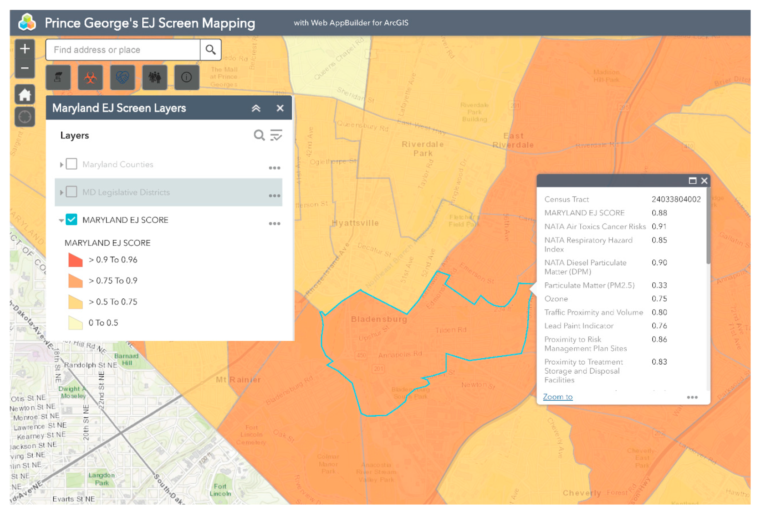
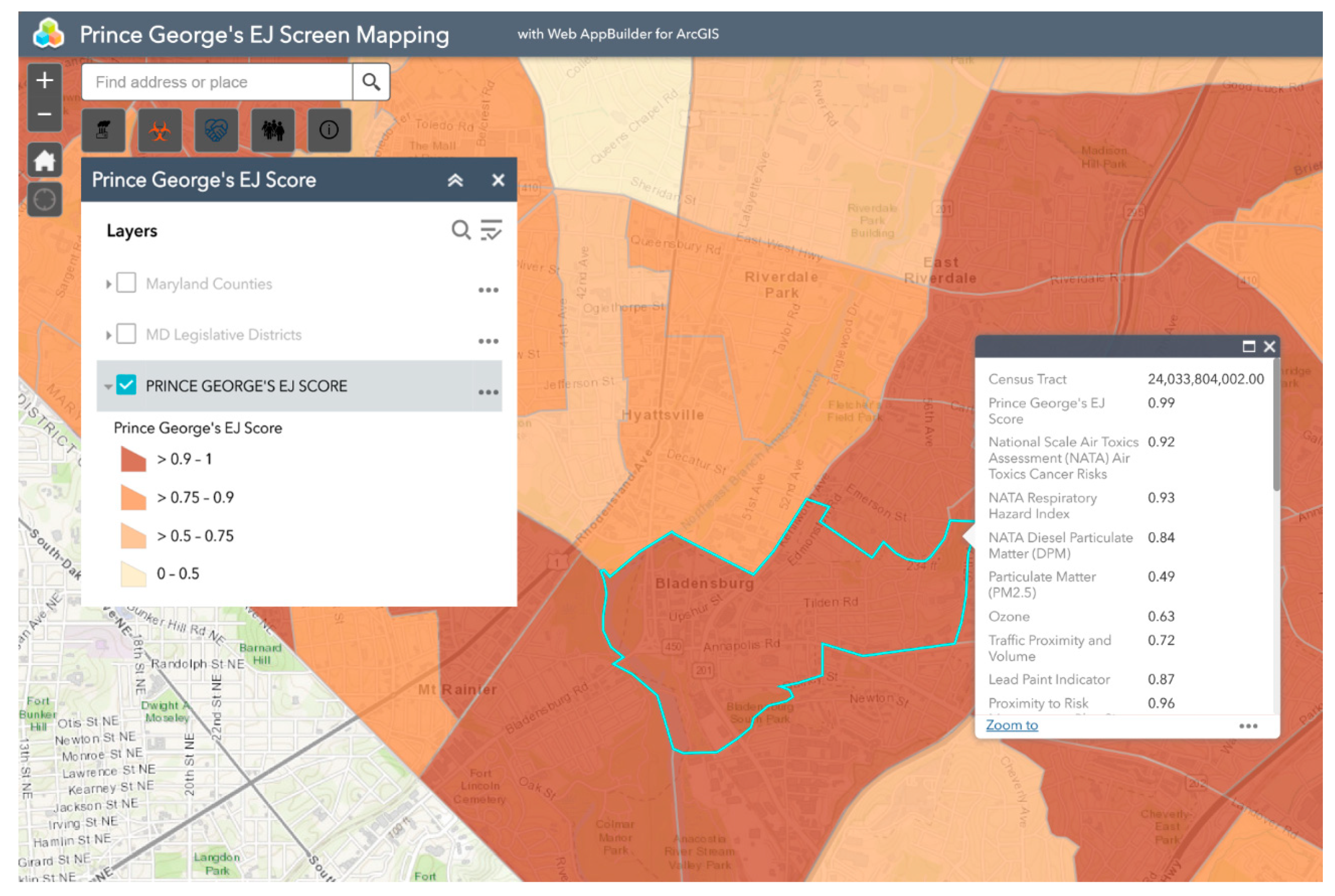
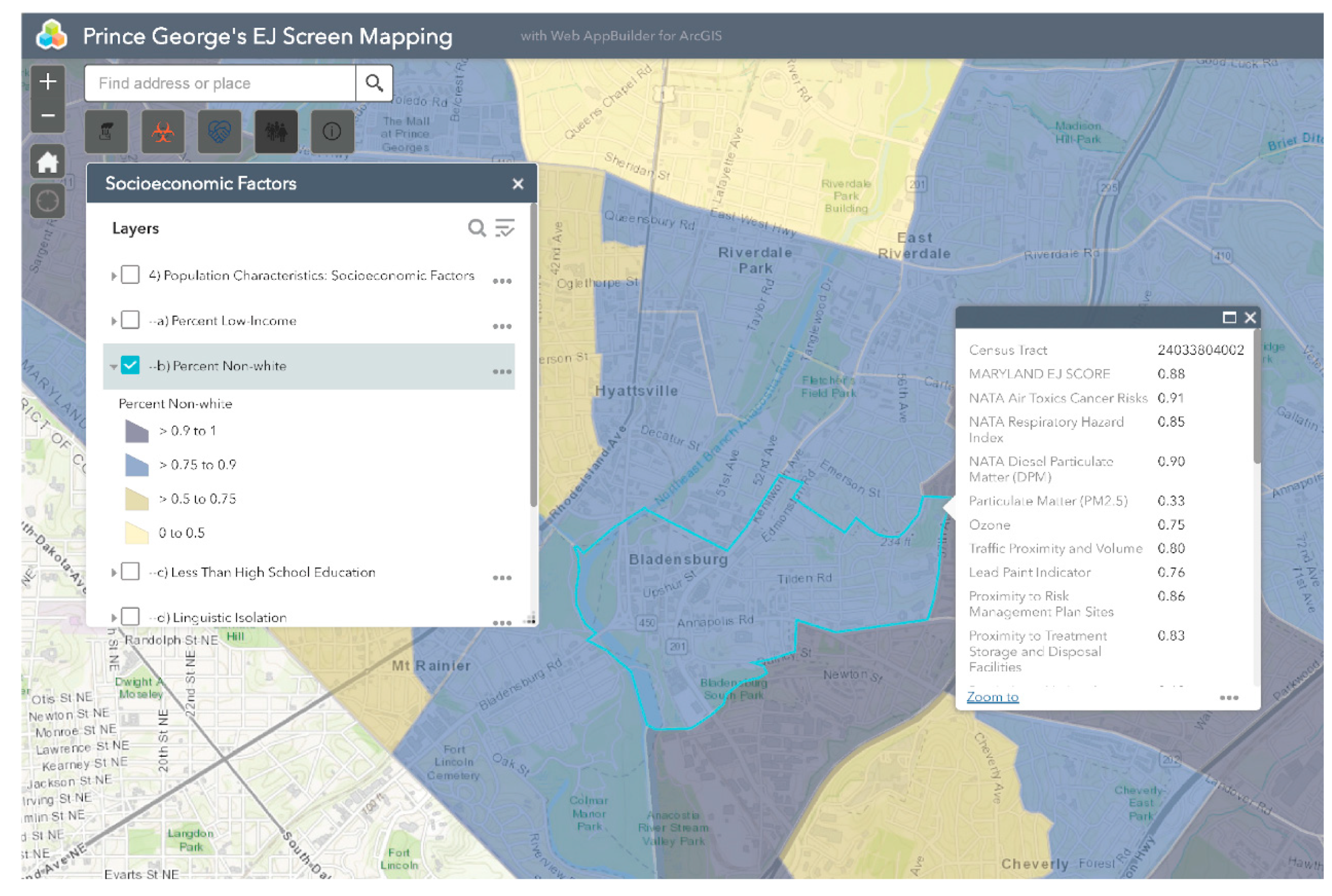
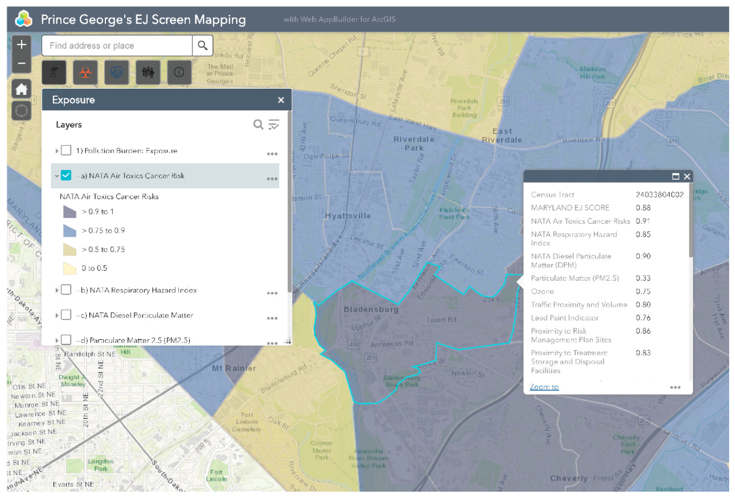
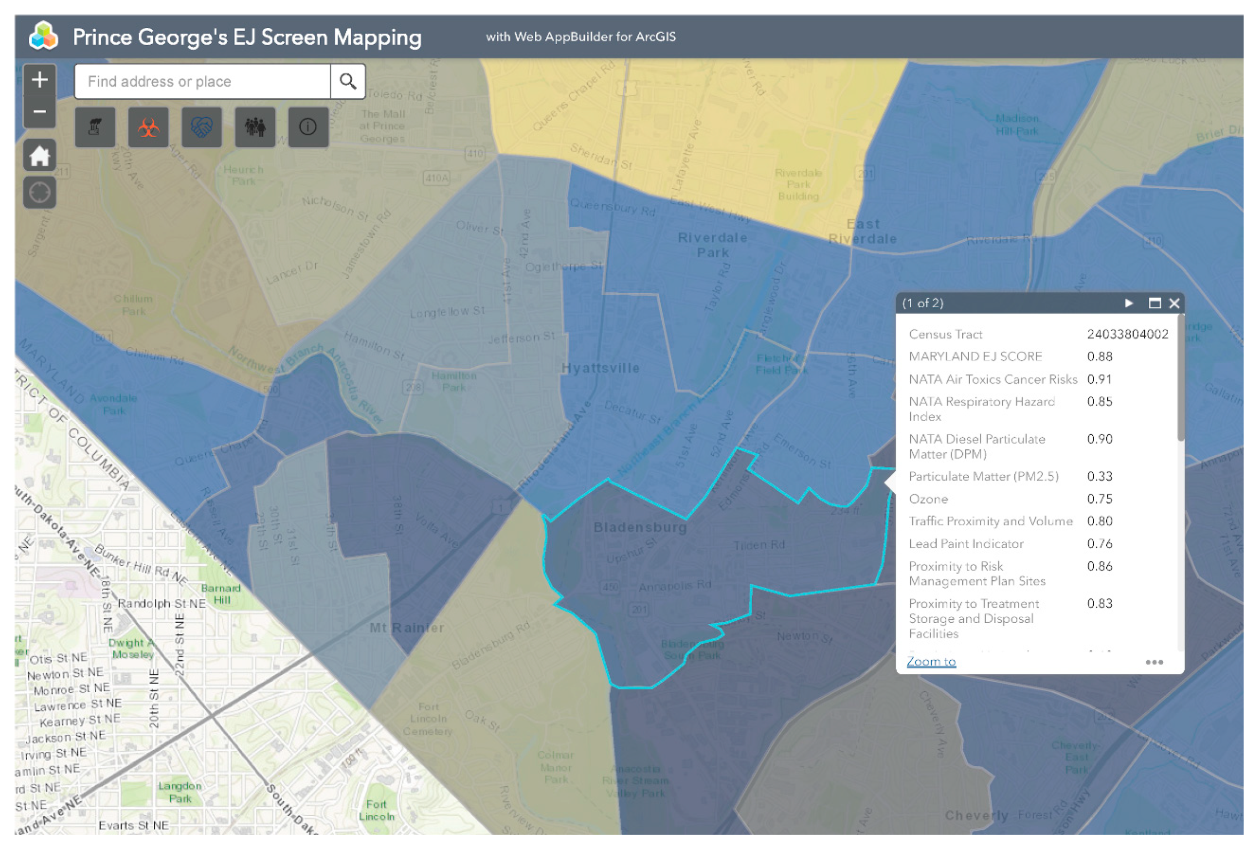
3.3. Bladensburg: A Case Study

Bladensburg is a town in Prince George’s County that has experienced environmental injustice due to racial and economic stratification. The Bladensburg population is primarily Black (62.7%) and Latinx (33.0%), with small concentrations of White (13.9%) and Asian (1.6%) residents [66]. Studies have shown that proximity to hazards is directly related to race/ethnicity, with one study specific to Maryland, Louisiana, and West Virginia finding that African-Americans are more likely to be located in close proximity to Toxic Release Inventory (TRI) facilities [67,68,69,70,71]. In comparison to the national average of 14%, 20.1% of Bladensburg residents live below the federal poverty line [66]. Due to underlying social and economic vulnerabilities, residents in Bladensburg are more likely to experience low property values and the disproportionate siting of environmental hazards in their communities than their more affluent counterparts [72,73]. Bladensburg residents also endure a large pollution burden, with heavy commuter and industrial traffic and a concrete block plant acting as sources of particulate matter (PM), volatile organic compounds (VOCs), and polycyclic aromatic hydrocarbons (PAHs) [74]. Due to their exposure to air pollutants, Bladensburg residents are at increased risk for respiratory problems and cancer [72,75,76,77]. An example analysis of environmental injustice in Bladensburg using MD EJSCREEN is presented below (Figure 2, Figure 3, Figure 4, Figure 5 and Figure 6). For the purpose of the Bladensburg case study, the PG EJ score, a separate score created by the tool, is used, in addition to the MD EJ score (Figure 2). The PG EJ score compares the Bladensburg census tract to the rest the census tracts in Prince George’s County, while the MD EJ score compares the Bladensburg census tract to all census tracts in Maryland. A comparison with EPA EJSCREEN is provided for Bladensburg in Figure 7.
For example, this map illustrates the PG EJ score for Bladensburg. The PG EJ score is represented as a percentile, meaning that Bladensburg has an EJ score higher than 99% of the census tracts in Prince George’s County. Furthermore, the score is an overall indication of the prevalence of environmental hazards in the Bladensburg area.
This map visualizes the percent non-White population in Bladensburg. Bladensburg appears within the 0.75–0.90 percentile range, meaning that its percent non-White population is higher than 75–90% of the census tracts in the state or county.
This map visualizes NATA air toxics cancer risk in Bladensburg. Bladensburg appears within the 0.9–1 percentile range, meaning that its NATA air toxics cancer risk is higher than 90–100% of the census tracts in the state or county.
This map visualizes the percent non-White population in Bladensburg in relation to NATA air toxics cancer risk. Bladensburg appears within the 0.9–1.0 percentile range, meaning that the calculated risk of developing cancer due to air pollution is higher than the risk in 90–100% of the census tracts in the state or county. Coupled with the high percentage non-White population, these findings illustrate the disproportionate exposure to human and environmental health hazards experienced by populations of color.
While MD EJSCREEN conducts analyses at a larger scale by organizing data by census tract, EPA EJSCREEN analyzes data on a smaller scale, by block group. According to Figure 7, this block group is 97% non-White and it is in the 95th percentile. This means that the percent non-White in this block group is greater than or equal to the percent non-White where 95% of the US population lives. The lifetime NATA cancer risk for this block group is 55 people per 1 million. This area is also in the 92nd percentile, meaning that the lifetime NATA cancer risk in this block group is greater than or equal to the risk where 92% of the US population lives.

4. Discussion

Despite the presence of tools such as EPA EJSCREEN and CalEnviroScreen, stakeholders expressed the need for a mapping tool which caters to specific environmental health concerns in Maryland. Other EJ mapping tools lack pertinent information on indicators specific to Maryland communities such as lead paint prevalence, NATA respiratory hazard index, and proximity to RMP sites. EPA EJSCREEN can map useful demographic and environmental indicators, but is hindered by its broad scope, and the use of block groups as the geographic unit of analysis.
EPA EJSCREEN was not developed with the intention of determining the presence or absence of environmental injustice in communities. All conclusions drawn from the tool must be substantiated with additional information at the local level in order to perform a true assessment of environmental justice. Due to the broad scope of the tool, it is unable to address all issues relevant at the local level. Therefore, many environmental concerns central to communities are not shown.
EPA EJSCREEN also identifies marginal uncertainty in EJ Index values when mapping block groups. Mapping an individual block group can identify pollution ‘hot spots’, but produces uncertainty because the tool must estimate the location of residences. Due to such uncertainties, the tool cannot confidently compare or rank indicators when only minor differences exist between percentile scores. In order to avoid such uncertainties, the US EPA recommends that users create a buffer by applying the tool to a larger geographic area that covers multiple block groups, but which may overlook ‘hot spots’ [36]. We seek to address this weakness in MD EJSCREEN by conducting analysis at a larger scale (using a census tract), rather than by block group.
As mentioned previously, only CalEnviroScreen and MD EJSCREEN are able to produce EJ scores for a user-specified census tract. The computation of an EJ score allows for clear and succinct analysis of the level of environmental injustice in an area of concern. EPA EJSCREEN cannot produce cumulative EJ scores but does produce EJ indices. An EJ index combines demographic indicators with a single environmental indicator, resulting in 11 EJ indexes that reflect the 11 environmental indicators in the tool. EJ indexes apply the idea of ‘excess risk’ by examining the disparities between block group averages and nation averages for environmental indicators across different demographic indicators. EJ indices can therefore be used to identify geographic locations which may burdened by environmental hazards. Despite this, EJ indices are limited in their applications to environmental justice because they do not consider the cumulative impacts of multiple environmental stressors on the health and well-being of a population.
Research has repeatedly shown that the concentration of environmental hazards elevates stress and other adverse health outcomes, while simultaneously decreasing quality of life and community sustainability [8,78,79,80]. Environmental stressors include water contamination, hazardous waste, land used for incinerators and landfills, and lack of green space [78]. MD EJSCREEN provides a more accessible and interactive way for residents to grasp how their health is affected by the built environment, visualize trends in who is directly affected and to what degree, and create long-lasting change in their community.
The US EPA has set environmental health standards, yet, these programs have not specifically confronted the issue of cumulative impacts on non-White populations [81]. This makes mapping tools such as EJSCREEN, CalEnviroScreen, and MD EJSCREEN significant in determining how populations of color suffer an unjust burden of environmental risks. The scores available in MD EJSCREEN allow residents and other stakeholders to compare the rates of pollution, the effects of pollution, and the most vulnerable subpopulations to other areas of the state. For instance, users can easily visualize that areas with a higher percentage of low-income residents also tend to be located near areas with high traffic volume and PM2.5, as well as the potential health risks associated with those locations [81]. These scores can be used by residents to better advocate for their health, and government officials to determine specific changes that need be made to reduce environmental injustice.
The ability of MD EJSCREEN to identify areas of environmental justice concern has been mirrored by other tools such as CalEnviroScreen. Researchers utilizing this technology found that non-White individuals are more likely to live near pollution sources than non-Hispanic Whites, and that they also experience higher concentrations of poverty, ozone, DPM, pesticide use, solid waste sites, and gas-fired power plants [8,82]. Additional studies isolating the Latinx population found that they are especially vulnerable to environmental injustice due factors such as linguistic isolation, racial segregation, systematic housing market discrimination, real estate steering practices, and blocked channels of residential and economic mobility [83,84]. Additionally, socioeconomic indicators such as education and income were found to be strongly associated with levels of disease burden [10,85].
CalEnviroScreen has also been used to link vulnerable populations to visionary policies capable of transforming overburdened areas into healthy, thriving communities. For example, California Environmental Justice Alliance (CEJA)’s Green Zones project applies the CalEnviroScreen tool to identify concentrations of industrial pollution sources thereby streamlining resources, regulatory attention, and sustainable economic development to vulnerable communities [86]. The term ‘Green Zone’, refers to mostly low-income communities of color that have organized against discriminatory land use patterns and for neighborhood restoration that addresses economic, social, and environmental health concerns [86].
The EPA’s Clean Power Plan employed EPA EJSCREEN to inform policy that addresses the disproportionate siting of environmental hazards in communities of color, low income, and indigenous communities by performing proximity-based analyses of power plants, taking into account demographics and cumulative impacts [87]. The analyses revealed that in comparison to nation averages, low income and people of color are more likely to live near power plants [83]. The proximity analysis outlined by the Clean Power Plan allows states to improve access to energy efficiency (EE), renewable energy (RE), and financial assistance programs [87].
Similarly, the North Carolina Department of Environmental Quality (NC DEQ) conducted an environmental justice assessment using EPA EJSCREEN for a proposed fly ash project at the Duke Energy Lee plant in Goldsboro, North Carolina. The EPA EJSCREEN analysis revealed that the per capita income of individuals living within two miles of the Lee plant is $17,847 per year, less than the Goldsboro average of $19,243, and the state average of $26,779. This information demonstrates that if the plant is to expand, the pollution burden would fall primarily on low-income communities [88].
EPA EJSCREEN has also been used to address the environmental health concerns of incarcerated populations. Currently, the tool is at the forefront of the ‘prison ecology movement’, which utilizes GIS mapping to examine the proximity of correctional facilities to known hazardous waste sites [89]. Studies performed by the Prison Ecology Project (PEP) found that among a range of federal and state prisons from Colorado to Indiana, 589 were located within three miles of a Superfund or hazardous waste site [90].
In conducting this study, we encountered multiple barriers to obtaining reliable feedback on the indicators. The amount of information we received for each indicator was not as complete as it could have been due to low response rates from stakeholders. Other limitations include the accuracy of the feedback received during the stakeholder meeting held in Bladensburg, Maryland. Due to these limitations, the utility of the additional indicators included within the ‘Additional Context’ category to the Prince George’s community, may be lower than anticipated. Nevertheless, the findings of this study can be further implemented in various future EJ investigations.
Presently, we are working to increase the functionality and usability of MD EJSCREEN so it has similar capabilities to EPA EJSCREEN and CalEnviroScreen particularly geostatistical analysis. In the future, we will add the ability of users to upload their own qualitative or quantitative data collected via citizen science or another scientific approach. Additionally, MD EJSCREEN will be expanded to the entire state of Maryland, enabling more communities to engage with and take control of environmental justice in their neighborhoods. As the tool expands, more pertinent indicators specific to Maryland could be incorporated based on feedback from stakeholders across the state, strengthening the tool and its ability to combat environmental injustice. Although no stakeholder evaluations have been conducted yet, once the tool is in its final stage of development, we will perform an evaluation of stakeholder satisfaction with the tool. These evaluations will focus on the major metrics used to assess the functionality and usability of GIS mapping tools. This will allow us to understand if the tool has achieved its primary objective: to represent the environmental justice concerns specific to Maryland residents.

5. Conclusions

MD EJSCREEN can be used to make public health improvements for all communities, allowing residents to advocate for new policies and better enforcement of policies. In addition, government officials can use the information provided by this tool to identify pressing concerns of their constituents and implement more equitable policies. A comprehensive training guide and video showing how to navigate and use the tool will be developed and released for community members and stakeholders. A series of training sessions will serve to provide technical assistance on an as-needed basis, making it easier to apply MD EJSCREEN in policy decisions and community advocacy.

Author Contributions

A.D., conceptualization, methodology, investigation, formal analysis, validation, original draft preparation, writing—review and editing; C.M., investigation, validation, formal analysis, visualization, writing—review and editing; S.B.-G., conceptualization, methodology, formal analysis, writing--original draft preparation; C.B., formal analysis, methodology, supervision, visualization, writing—review and editing; J.L., formal analysis, investigation, visualization, writing—review and editing; S.W., conceptualization, methodology, project administration, funding acquisition, writing—review and editing.

Funding

This research was funded by the National Center for Smart Growth’s Partnership for Action Learning in Sustainability (PALS).

Acknowledgments

We would like to acknowledge Daniel Engelberg, from the National Center for Smart Growth, the Partnerships in Action Learning in Sustainability (PALS), and the Prince George’s County Department of the Environment (DOE) for their support of this project. We would also like to acknowledge the contribution of Haley Mullen, Vivek Ravichandran, Wengiel Gugssa, Maddie Hagerty, Vanessa Tellez, Skylar Petrik, Root Woldu, and Asher Moldwin to the project.

Conflicts of Interest

The authors declare no conflict of interest. The funders had no role in the design of the study; in the collection, analyses, or interpretation of data; in the writing of the manuscript, or in the decision to publish the results.

References

  1. Adamkiewicz, G.; Spengler, J.D.; Harley, A.E.; Stoddard, A.; Yang, M.; Alvarez-Reeves, M.; Sorensen, G. Environmental conditions in low-income urban housing: Clustering and associations with self-reported health. Am. J. Public Health 2014, 104, 1650–1656. [Google Scholar] [CrossRef]
  2. Koester, S.; Davis, S. Siting of Wood Pellet Production Facilities in Environmental Justice Communities in the Southeastern United States. Environ. Justice 2018, 11, 64–70. [Google Scholar] [CrossRef]
  3. Johnston, J.E.; Werder, E.; Sebastian, D. Wastewater Disposal Wells, Fracking, and Environmental Injustice in Southern Texas. Am. J. Public Health 2016, 106, 550–556. [Google Scholar] [CrossRef] [Green Version]
  4. Stretesky, P.B.; McKie, R. A perspective on the historical analysis of race and treatment storage and disposal facilities in the United States. Environ. Res. Lett. 2016, 11, 031001. [Google Scholar] [CrossRef] [Green Version]
  5. Schulz, A.J.; Mentz, G.B.; Sampson, N.; Ward, M.; Anderson, R.; de Majo, R.; Israel, B.A.; Lewis, T.C.; Wilkins, D. Race and the distribution of social and physical environmental risk: A Case Example from the Detroit Metropolitan Area. Du Bois Rev. Soc. Sci. Res. Race 2016, 13, 285–304. [Google Scholar] [CrossRef]
  6. Mohai, P.; Saha, R. Which came first, people or pollution? Assessing the disparate siting and post-siting demographic change hypotheses of environmental injustice. Environ. Res. Lett. 2015, 10, 115008. [Google Scholar] [CrossRef] [Green Version]
  7. Ard, K. Trends in exposure to industrial air toxins for different racial and socioeconomic groups: A spatial and temporal examination of environmental inequality in the U.S. from 1995 to 2004. Soc. Sci. Res. 2015, 53, 375–390. [Google Scholar] [CrossRef]
  8. Cushing, L.; Faust, J.; August, L.M.; Cendak, R.; Wieland, W.; Alexeeff, G. Racial/Ethnic Disparities in Cumulative Environmental Health Impacts in California: Evidence from a Statewide Environmental Justice Screening Tool (CalEnviroScreen 1.1). Am. J. Public Health 2015, 105, 2341–2348. [Google Scholar] [CrossRef]
  9. Brender, J.D.; Maantay, J.A.; Chakraborty, J. Residential Proximity to Environmental Hazards and Adverse Health Outcomes. Am. J. Public Health 2011, 101, S37–S52. [Google Scholar] [CrossRef] [Green Version]
  10. Greenfield, B.K.; Rajan, J.; McKone, T.E. A multivariate analysis of CalEnviroScreen: Comparing environmental and socioeconomic stressors versus chronic disease. Environ. Health 2017, 16, 131. [Google Scholar] [CrossRef]
  11. Jerrett, M.; Burnett, R.; Brook, J.; Kanaroglou, P.; Giovis, C.; Finkelstein, N.; Hutchison, B. Do socioeconomic characteristics modify the short term association between air pollution and mortality? Evidence from a zonal time series in Hamilton, Canada. J. Epidemiol. Community Health 2004, 58, 31–40. [Google Scholar] [CrossRef] [Green Version]
  12. Wilson, S.M. An Ecologic Framework to Study and Address Environmental Justice and Community Health Issues. Environ. Justice 2009, 2, 15–24. [Google Scholar] [CrossRef]
  13. Maantay, J. Asthma and air pollution in the Bronx: Methodological and data considerations in using GIS for environmental justice and health research. Health Place 2007, 13, 32–56. [Google Scholar] [CrossRef]
  14. Sadd, J.L.; Pastor, M.; Morello-Frosch, R.; Scoggins, J.; Jesdale, B. Playing It Safe: Assessing Cumulative Impact and Social Vulnerability through an Environmental Justice Screening Method in the South Coast Air Basin, California. Int. J. Environ. Res. Public Health 2011, 8, 1441–1459. [Google Scholar] [CrossRef] [Green Version]
  15. Jerrett, M.; Burnett, R.T.; Kanaroglou, P.; Eyles, J.; Finkelstein, N.; Giovis, C.; Brook, J.R. A GIS–Environmental Justice Analysis of Particulate Air Pollution in Hamilton, Canada. Environ. Plan. A 2001, 33, 955–973. [Google Scholar] [CrossRef]
  16. Morello-Frosch, R.; Pastor, M.; Sadd, J. Environmental Justice and Southern California’s “Riskscape”: The Distribution of Air Toxics Exposures and Health Risks among Diverse Communities. Urban Aff. Rev. 2001, 36, 551–578. [Google Scholar] [CrossRef]
  17. Bellander, T.; Berglind, N.; Gustavsson, P.; Jonson, T.; Nyberg, F.; Pershagen, G.; Järup, L. Using geographic information systems to assess individual historical exposure to air pollution from traffic and house heating in Stockholm. Environ. Health Perspect. 2001, 109, 633–639. [Google Scholar] [CrossRef]
  18. Nuvolone, D.; della Maggiore, R.; Maio, S.; Fresco, R.; Baldacci, S.; Carrozzi, L.; Pistelli, F.; Viegi, G. Geographical information system and environmental epidemiology: A cross-sectional spatial analysis of the effects of traffic-related air pollution on population respiratory health. Environ. Health 2011, 10, 12. [Google Scholar] [CrossRef]
  19. Nyberg, F.; Gustavsson, P.; Järup, L.; Bellander, T.; Berglind, N.; Jakobsson, R.; Pershagen, G. Urban Air Pollution and Lung Cancer in Stockholm. Epidemiology 2000, 11, 487–495. [Google Scholar] [CrossRef] [Green Version]
  20. Jelks, N.; Hawthorne, T.; Dai, D.; Fuller, C.; Stauber, C.; Jelks, N.O.; Hawthorne, T.L.; Dai, D.; Fuller, C.H.; Stauber, C. Mapping the Hidden Hazards: Community-Led Spatial Data Collection of Street-Level Environmental Stressors in a Degraded, Urban Watershed. Int. J. Environ. Res. Public Health 2018, 15, 825. [Google Scholar] [CrossRef]
  21. Cutts, B.B.; Darby, K.J.; Boone, C.G.; Brewis, A. City structure, obesity, and environmental justice: An integrated analysis of physical and social barriers to walkable streets and park access. Soc. Sci. Med. 2009, 69, 1314–1322. [Google Scholar] [CrossRef]
  22. Frank, L.; Glanz, K.; McCarron, M.; Sallis, J.; Sealens, B.; Chapman, J. The Spatial Distribution of Food Outlet Type and Quality around Schools in Differing Built Environment and Demographic Contexts. Berkeley Plan. J. 2006, 19, 79–95. [Google Scholar]
  23. Larsen, K.; Gilliland, J. Mapping the evolution of “food deserts” in a Canadian city: Supermarket accessibility in London, Ontario, 1961–2005. Int. J. Health Geogr. 2008, 7, 16. [Google Scholar] [CrossRef]
  24. Jiao, Y.; Bower, J.; Im, W.; Basta, N.; Obrycki, J.; Al-Hamdan, M.; Wilder, A.; Bollinger, C.; Zhang, T.; Hatten, L.; et al. Application of Citizen Science Risk Communication Tools in a Vulnerable Urban Community. Int. J. Environ. Res. Public Health 2015, 13, 11. [Google Scholar] [CrossRef]
  25. London, J.K.; Zagofsky, T.M.; Huang, G.; Saklar, J. Collaboration, Participation and Technology: The San Joaquin Valley Cumulative Health Impacts Project. Gateways 2011, 4, 12–30. [Google Scholar] [CrossRef] [Green Version]
  26. Ghose, R.; Elwood, S. Public Participation GIS and Local Political Context: Propositions and Research Directions. Urisa J. 2003, 15, 17–22. [Google Scholar]
  27. Sun, M.T.-W.; Tsai, Y.-T.; Shih, M.-C.; Lin, J.Y.-W. Public participation and the concept of space in environmental governance: An application of PPGIS. Public Adm. Dev. 2009, 29, 250–261. [Google Scholar] [CrossRef]
  28. Sieber, R. Public Participation Geographic Information Systems: A Literature Review and Framework. Ann. Assoc. Am. Geogr. 2006, 96, 491–507. [Google Scholar] [CrossRef] [Green Version]
  29. Huang, G.; London, J.K. Mapping in and out of “messes”: An adaptive, participatory, and transdisciplinary approach to assessing cumulative environmental justice impacts. Landsc. Urban Plan. 2016, 154, 57–67. [Google Scholar] [CrossRef]
  30. Raymond, C.M.; Gottwald, S.; Kuoppa, J.; Kyttä, M. Integrating multiple elements of environmental justice into urban blue space planning using public participation geographic information systems. Landsc. Urban Plan. 2016, 153, 198–208. [Google Scholar] [CrossRef]
  31. Laatikainen, T.; Tenkanen, H.; Kyttä, M.; Toivonen, T. Comparing conventional and PPGIS approaches in measuring equality of access to urban aquatic environments. Landsc. Urban Plan. 2015, 144, 22–33. [Google Scholar] [CrossRef]
  32. Brown, G.; Schebella, M.F.; Weber, D. Using participatory GIS to measure physical activity and urban park benefits. Landsc. Urban Plan. 2014, 121, 34–44. [Google Scholar] [CrossRef]
  33. Brown, G.G.; Reed, P. Public Participation GIS: A New Method for Use in National Forest Planning. For. Sci. 2009, 55, 166–182. [Google Scholar]
  34. Brown, G.; Weber, D.; de Bie, K. Is PPGIS good enough? An empirical evaluation of the quality of PPGIS crowd-sourced spatial data for conservation planning. Land Use Policy 2015, 43, 228–238. [Google Scholar] [CrossRef]
  35. Faust, J.; Laura, A.; Komal, B.; Vanessa, G.; Julian, L.; Shankar, P.; Rose, S.; Andrew, S.; Robbie, W.; Walker, W.; et al. Update to the California Communities Environmental Health Screening Tool CalEnviroScreen 3.0; CalEPA: Sacramento, CA, USA, 2017. [Google Scholar]
  36. Office of Policy, U.S. Environmental Protection Agency. EJSCREEN Technical Document. Available online: https://www.epa.gov/sites/production/files/2017-09/documents/2017_ejscreen_technical_document.pdf (accessed on 13 November 2018).
  37. Kuruppuarachchi, L.N.; Kumar, A.; Franchetti, M. A Comparison of Major Environmental Justice Screening and Mapping Tools. Environ. Manag. Sustain. Dev. 2017, 6, 59–71. [Google Scholar] [CrossRef]
  38. Office of Environmental Health Hazard Assessment, California Environmental Protection Agency Scoring & Model. Available online: https://oehha.ca.gov/calenviroscreen/scoring-model (accessed on 2 November 2018).
  39. Knaap, G. Technical Memorandum #2: Measures of Opportunity in the Baltimore Metropolitan Region 2013. Available online: http://smartgrowth.umd.edu/assets/documents/sci_tech_memo_2.pdf (accessed on 24 January 2019).
  40. Office of Environmental Health Hazard Assessment Population Indicators. Available online: https://oehha.ca.gov/calenviroscreen/population-indicators (accessed on 20 November 2018).
  41. Wilson, S.; Hutson, M.; Mujahid, M. How Planning and Zoning Contribute to Inequitable Development, Neighborhood Health, and Environmental Injustice. Environ. Justice 2008, 1, 211–216. [Google Scholar] [CrossRef]
  42. Galvin, M.F.; Grove, J.M.; O’Neil-Dunne, J.P.M.; Todd, A.; Clagett, S. Urban Tree Canopy Goal Setting; United States Department of Agriculture: Washington, DC, USA, 2015.
  43. Solid Waste and Emergency Response, U.S. Environmental Protection Agency. EPA Targeted Brownfields Assessments the Basics; U.S. Environmental Protection Agency: Washington, DC, USA, 2015.
  44. Office of Water, U.S. Environmental Protection Agency. Wetlands Overview; U.S. Environmental Protection Agency: Washington, DC, USA, 2004.
  45. Nonpoint Source Program, Maryland Department of the Environment. Maryland’s 2015–2019 Nonpoint Source Management Plan; Nonpoint Source Program, Maryland Department of the Environment: Baltimore, MD, USA, 2016.
  46. Uphoff, E.P.; Pickett, K.E.; Cabieses, B.; Small, N.; Wright, J. A systematic review of the relationships between social capital and socioeconomic inequalities in health: A contribution to understanding the psychosocial pathway of health inequalities. Int. J. Equity Health 2013, 12, 54. [Google Scholar] [CrossRef]
  47. BorisRachel, E.T.; Mosher-Williams, R. Nonprofit Advocacy Organizations: Assessing the Definitions, Classifications, and Data. Nonprofit & Voluntary Sector Q. 1998, 27, 488–506. [Google Scholar]
  48. U.S. Census Bureau. Industry Statistics Portal: NAICS Grocery Stores. Available online: https://www.census.gov/econ/isp/sampler.php?naicscode=445110&naicslevel=6# (accessed on 17 November 2018).
  49. U.S. Census Bureau. Industry Statistics Portal: NAICS Convenience Stores. Available online: https://www.census.gov/econ/isp/sampler.php?naicscode=44512&naicslevel=5# (accessed on 17 November 2018).
  50. U.S. Census Bureau. Industry Statistics Portal: NAICS Liquor Stores. Available online: https://www.census.gov/econ/isp/sampler.php?naicscode=4453&naicslevel=4# (accessed on 17 November 2018).
  51. Prince George’s County Planning Department. Industrial Zones. Available online: http://www.pgparks.com/833/Industrial-Zones (accessed on 17 November 2018).
  52. GreenInfo Network; Great Basin Cooperative Ecosystem Studies Unit, Boise State University. Completing America’s Inventory of Public Parks and Protected Areas. Available online: http://www.protectedlands.net/wp-content/uploads/2014/09/ParksOpenSpace_PolicyPaperNov2016Final.pdf (accessed on 17 November 2018).
  53. Prince George’s County Planning Department. Comprehensive Design. Available online: http://www.pgparks.com/813/Comprehensive-Design (accessed on 17 November 2018).
  54. Office of Water, U.S. Environmental Protection Agency. Clean Water Act, Section 502 General Definitions. Available online: https://www.epa.gov/cwa-404/clean-water-act-section-502-general-definitions (accessed on 2 November 2018).
  55. Office of Air and Radiation, U.S. Environmental Protection Agency. Pollutants and Sources|Technology Transfer Network Air Toxics Web Site|US EPA. Available online: https://www3.epa.gov/airtoxics/pollsour.html (accessed on 2 November 2018).
  56. Office of Air and Radiation, U.S. Environmental Protection Agency. True Minor Source and Synthetic Minor Source Permits. Available online: https://www.epa.gov/tribal-air/true-minor-source-and-synthetic-minor-source-permits (accessed on 2 November 2018).
  57. Office of Resource Conservation and Recovery, U.S. Environmental Protection Agency. Defining Hazardous Waste: Listed, Characteristic and Mixed Radiological Wastes. Available online: https://www.epa.gov/hw/defining-hazardous-waste-listed-characteristic-and-mixed-radiological-wastes (accessed on 17 November 2018).
  58. Health Resources and Services Administration. Health Professional Shortage Areas (HPSAs). Available online: https://bhw.hrsa.gov/shortage-designation/hpsas (accessed on 2 November 2018).
  59. Statistics Canada. NAICS 2012-44511-Supermarkets and Other Grocery (Except Convenience) Stores. Available online: http://www23.statcan.gc.ca/imdb/p3VD.pl?Function=getVD&TVD=118464&CVD=118468&CPV=44511&CST=01012012&CLV=4&MLV=5 (accessed on 2 November 2018).
  60. The Reinvestment Fund. 2014 Analysis of Limited Supermarket Access Summary Brief; The Reinvestment Fund: Philadelphia, PA, USA, 2015. [Google Scholar]
  61. U.S. National Library of Medicine, Department of Health and Human Services. What Are the Superfund site “NPL” Statuses? Available online: https://toxmap.nlm.nih.gov/toxmap/faq/2009/08/what-are-the-superfund-site-npl-statuses.html (accessed on 2 November 2018).
  62. Prince George’s County Public Schools List of All Schools. Available online: https://www.pgcps.org/list-of-schools-by-type/ (accessed on 21 January 2019).
  63. Technology Transformation Service, U.S.G.S.A. 2015 Nation US Rails National Shapefile. Available online: https://catalog.data.gov/dataset/tiger-line-shapefile-2015-nation-u-s-rails-national-shapefile (accessed on 21 January 2019).
  64. Khan, Z.A.; Adnan, M. Usability Evaluation of Web-based GIS Applications; Blekinge Institute of Technology: Karlskrona, Sweden, 2010. [Google Scholar]
  65. Jokela, T.; Iivari, N.; Matero, J.; Karukka, M. The Standard of User-centered Design and the Standard Definition of Usability: Analyzing ISO 13407 Against ISO 9241-11. In Proceedings of the Latin American Conference on Human-Computer Interaction, Rio de Janeiro, Brazil, 17–20 August 2003; ACM: New York, NY, USA, 2003; pp. 53–60. [Google Scholar]
  66. U.S. Census Bureau American FactFinder. Available online: https://factfinder.census.gov/faces/nav/jsf/pages/index.xhtml (accessed on 8 August 2018).
  67. Zwickl, K.; Ash, M.; Boyce, J.K. Regional variation in environmental inequality: Industrial air toxics exposure in U.S. cities. Ecol. Econ. 2014, 107, 494–509. [Google Scholar] [CrossRef] [Green Version]
  68. Downey, L. US Metropolitan-area Variation in Environmental Inequality Outcomes. Urban Stud. 2007, 44, 953–977. [Google Scholar] [CrossRef] [Green Version]
  69. Sicotte, D. Diversity and Intersectionality among Environmentally Burdened Communities in the Philadelphia Metropolitan Area, USA. Urban Stud. 2014, 51, 1850–1870. [Google Scholar] [CrossRef]
  70. Pastor, M.; Sadd, J.L.; Morello-Frosch, R. Reading, Writing, and Toxics: Children’s Health, Academic Performance, and Environmental Justice in Los Angeles. Environ. Plan. C Gov. Policy 2004, 22, 271–290. [Google Scholar] [CrossRef]
  71. Perlin, S.A.; Wong, D.; Sexton, K. Residential proximity to industrial sources of air pollution: Interrelationships among race, poverty, and age. J. Air Waste Manag. Assoc. 2001, 51, 406–421. [Google Scholar] [CrossRef]
  72. Bell, M.L.; Zanobetti, A.; Dominici, F. Evidence on vulnerability and susceptibility to health risks associated with short-term exposure to particulate matter: A systematic review and meta-analysis. Am. J. Epidemiol. 2013, 178, 865–876. [Google Scholar] [CrossRef]
  73. Stuart, A.L.; Mudhasakul, S.; Sriwatanapongse, W. The social distribution of neighborhood-scale air pollution and monitoring protection. J. Air Waste Manag. Assoc. 2009, 59, 591–602. [Google Scholar] [CrossRef]
  74. Bharti, S.K.; Trivedi, A.; Kumar, N. Air pollution tolerance index of plants growing near an industrial site. Urban Clim. 2018, 24, 820–829. [Google Scholar] [CrossRef]
  75. Ye, D.; Klein, M.; Chang, H.H.; Sarnat, J.A.; Mulholland, J.A.; Edgerton, E.S.; Winquist, A.; Tolbert, P.E.; Sarnat, S.E. Estimating Acute Cardiorespiratory Effects of Ambient Volatile Organic Compounds. Epidemiology 2017, 28, 197–206. [Google Scholar] [CrossRef]
  76. Raaschou-Nielsen, O.; Andersen, Z.; Hvidberg, M.; Jensen, S.; Ketzel, M.; Sørensen, M.; Loft, S.; Overvad, K.; Tjønneland, A. Lung Cancer Incidence and Long-Term Exposure to Air Pollution from Traffic. Environ. Health Perspect. 2011, 119, 860–865. [Google Scholar] [CrossRef] [Green Version]
  77. Ramírez, N.; Cuadras, A.; Rovira, E.; Borrull, F.; Marcé, R.M. Chronic risk assessment of exposure to volatile organic compounds in the atmosphere near the largest Mediterranean industrial site. Environ. Int. 2012, 39, 200–209. [Google Scholar] [CrossRef]
  78. Roelofs, C.; Baron, S.L.; Sacoby, W.; Aaron, A. Occupational and Environmental Health Equity and Social Justice. In Occupational and Environmental Health; Oxford University Press: Oxford, UK, 2017; pp. 23–40. ISBN 978-0-19-066268-4. [Google Scholar]
  79. Kelly, F.J.; Fussell, J.C. Linking ambient particulate matter pollution effects with oxidative biology and immune responses. Ann. N. Y. Acad. Sci. 2015, 1340, 84–94. [Google Scholar] [CrossRef]
  80. Ou, J.Y.; Peters, J.L.; Levy, J.I.; Bongiovanni, R.; Rossini, A.; Scammell, M.K. Self-rated health and its association with perceived environmental hazards, the social environment, and cultural stressors in an environmental justice population. BMC Public Health 2018, 18, 970. [Google Scholar] [CrossRef]
  81. Gladd, K.H. Air Toxics: EPA Action on Cumulative Impacts. Nat. Resour. Environ. Chic. 2017, 31, 51–53. [Google Scholar]
  82. Krieger, E.M.; Casey, J.A.; Shonkoff, S.B.C. A framework for siting and dispatch of emerging energy resources to realize environmental and health benefits: Case study on peaker power plant displacement. Energy Policy 2016, 96, 302–313. [Google Scholar] [CrossRef]
  83. Stewart, I.T.; Bacon, C.M.; Burke, W.D. The uneven distribution of environmental burdens and benefits in Silicon Valley’s backyard. Appl. Geogr. 2014, 55, 266–277. [Google Scholar] [CrossRef]
  84. Liévanos, R.S. Retooling CalEnviroScreen: Cumulative Pollution Burden and Race-Based Environmental Health Vulnerabilities in California. Int. J. Environ. Res. Public Health 2018, 15, 762. [Google Scholar] [CrossRef]
  85. Vieira, V.M.; Villanueva, C.; Chang, J.; Ziogas, A.; Bristow, R.E. Impact of community disadvantage and air pollution burden on geographic disparities of ovarian cancer survival in California. Environ. Res. 2017, 156, 388–393. [Google Scholar] [CrossRef]
  86. Eng, T.; Vanderwarker, A. Green Zones Across California; California Environmental Justice Alliance: Oakland, CA, USA, 2018; p. 36. [Google Scholar]
  87. Office of Air and Radiation, U.S. Environmental Protection Agency. EJ Screening Report for the Clean Power Plan; U.S. Environmental Protection Agency: Washington, DC, USA, 2015.
  88. Sorg, L. Dust-Up between DEQ, Advocates Over Environmental Justice Analysis at HF Lee Plant; Comment Period Ends Today; The Progressive Pulse: Raleigh, NC, USA, 2018. [Google Scholar]
  89. Bradshaw, E.A. Tombstone Towns and Toxic Prisons: Prison Ecology and the Necessity of an Anti-prison Environmental Movement. Crit. Crim. 2018, 26, 407–422. [Google Scholar] [CrossRef]
  90. Bernd, C.; Nandini, M.; Loftus-Farren, Z. America’s Toxic Prisons: The Environmental Injustices of Mass Incarceration. Available online: https://truthout.org/articles/america-s-toxic-prisons-the-environmental-injustices-of-mass-incarceration/ (accessed on 19 November 2018).
Figure 1. Overview of MD EJ (Maryland Environmental Justice) Scoring Process. The Environmental Exposure and the Environmental Effects Scores are averaged to calculate the Pollution Burden, and the Sensitive Populations and Socioeconomic Factors are averaged to create the Population Characteristics Score. The Pollution Burden and Population Characteristics are then multiplied to calculate the final MD EJ Score.
Ijerph 16 00348 g001
Figure 2. MD EJ Score for Bladensburg. This screenshot from the MD EJSCREEN mapping tool shows the MD EJ Score layer for Bladensburg, MD.
Ijerph 16 00348 g002
Figure 3. PG EJ score for Bladensburg. This screenshot from the MD EJSCREEN mapping tool shows the PG EJ score of Bladensburg, MD.
Ijerph 16 00348 g003
Figure 4. Percent non-White in Bladensburg. This map highlights the rate of percent non-White individuals in Bladensburg, MD.
Ijerph 16 00348 g004
Figure 5. NATA air toxics cancer risk in Bladensburg. This screenshot from the MD EJSCREEN mapping tool shows the percentile for the NATA air toxics cancer risk in Bladensburg, MD.
Ijerph 16 00348 g005
Figure 6. NATA air toxics layer overlaid with percent non-White in Bladensburg.
Ijerph 16 00348 g006
Figure 7. EPA EJSCREEN side-by-side maps displaying national percentiles for NATA air toxics cancer risk (left) and non-White population (right).
Ijerph 16 00348 g007
Table 1. Comparison of EJ (Environmental Justice) screening tool indicators.
IndicatorsDescriptionEPA EJSCREENCalEnviroScreenMD EJSCREEN
Pollution Burden: Exposure
National Scale Air Toxics Air (NATA) Toxics Cancer RiskLifetime risk of developing cancer from inhalation of air toxins. Reported as risk per lifetime per million people [36].X X
NATA Respiratory Hazard IndexAir toxics respiratory hazard index. This is the sum of hazard indices for those air toxics with reference concentrations based on respiratory endpoints, where each hazard index is the ratio of exposure concentration in the air to the health-based reference [36].X X
NATA Diesel Particulate Matter (DPM)Levels of diesel particulate matter in air. Reported as micrograms per cubic meter (µg/m3) [35,36].XXX
Particulate Matter (PM2.5)Levels of particulate matter with a diameter of 2.5 micrometers or smaller in air. Reported as micrograms per cubic meter (µg/m3) [35,36].XXX
OzoneSummer seasonal average of the maximum daily 8-hour concentration of ozone in air in parts per billion [35,36].XXX
Traffic Proximity and VolumeCount of vehicles (average annual daily traffic) at major roads within 500 meters or close to 500 meters, divided by distance in meters [35,36].XXX
Pesticide UseTotal pounds of selected active pesticide ingredients (filtered for hazard and volatility) used in production-agriculture per square mile, averaged over three years (2012 to 2014) [36]. X
Drinking Water ContaminantsWater tested to contain one or more contaminants listed in ‘Update to California Communities Environmental Health Screening Tool’. Reported as yearly averages of chemical contaminant concentrations for each census tract [36]. X
Toxic Releases from FacilitiesToxicity-weighted concentrations of modeled chemical releases to air from facility emissions and off-site incineration (averaged over 2011 to 2013) [36]. X
Pollution Burden: Environmental Effects
Lead Paint IndicatorPercent of houses built before 1960, which likely contain lead paint [36].X X
Proximity to Risk Management Plan (RMP) SitesCount of RMP (potential chemical accident management plans) facilities within 5 kilometers or close to 5 kilometers, divided by distance in kilometers [36].X X
Proximity to Treatment Storage and Disposal Facilities (TSDF)Count of TSDF (hazardous waste management facilities) within 5 kilometers or closest to 5 kilometers, divided by distance in kilometers [36].X X
Proximity to National Priorities List (NPL) SitesCount of NPL/Superfund sites (polluted sites that pose a risk to human health and/or the environment) within 5 kilometers or close to 5 kilometers, divided by distance in kilometers [35,36].XXX
Proximity to Major Direct Water DischargesToxic concentrations in stream segments within 500 meters, divided by distance in kilometers (km). Standards modeled after Risk-Screening Environmental Indicators (RSEI) [36].X X
Watershed FailurePercent of each census tract’s watershed that exceeds levels of phosphorus and/or nitrogen [39]. X
Groundwater ThreatNature and the magnitude of the threat and burden to groundwater safety posed by sites maintained in GeoTracker [35]. X
Impaired Water BodiesContamination of streams, rivers, and lakes by pollutants which compromise the ability to use a body of water for drinking, swimming, fishing, aquatic life protection, etc. [35]. X
Solid Waste Sites and FacilitiesSolid waste landfills, composting, and recycling facilities [35]. X
Population Characteristics: Sensitive Populations
Asthma Emergency DischargesCount of patients released from the hospital after being admitted for asthma or asthma-related distress [40]. X
Myocardial Infarction DischargesPatients released from the hospital after being admitted for a heart attack or heart attack symptoms [35]. XX
Low Birth Weight InfantsBabies born weighing less than 5.5 pounds [35]. XX
Asthma Emergency VisitsPatients admitted to the emergency room for asthma or asthma-related distress [35]. X
Population Characteristics: Socioeconomic Factors
Percent Non-WhitePercentage of individuals who define themselves as any race/ethnicity besides non-Hispanic White [35,36].XXX
Percent Low-IncomePercentage of individuals whose household income in the past 12 months is less than two times below the federal poverty level [35,36].XXX
Less than high school educationPercentage of individuals 25 and older who lack a high school diploma [35,36].XXX
Linguistic IsolationPercentage of households in which no one 14 years old and older speaks English "very well", or households which speak only English [35,36].XXX
Individuals under age 5Percentage of people under the age of 5 [36].X X
Individuals over age 64Percentage of people over the age of 64 [36].X X
UnemploymentPercentage of the population over the age of 16 that is unemployed and eligible for the labor force. Excludes retirees, students, homemakers, institutionalized persons except prisoners, those not looking for work, and military personnel on active duty [35]. XX
Housing Burdened Low Income HouseholdsPercentage of households in a census tract that make less than 80% of the HUD Area Median Family Income and paying greater than 50% of their income to finance housing [35]. X
Table 2. Additional indicators in MD EJSCREEN tool promoted by stakeholders.
IndicatorDescriptionData Source and Year
Pathogenic InfrastructureFeatures of the built environment that increase a population’s vulnerability to chemical and non-chemical stressors leading to adverse health outcomes. For example, liquor stores, fast food restaurants, convenience stores, pawn shops, and payday lenders [41].American Society of Civil Engineers (ASCE), 2017
Salutogenic InfrastructurePhysical, economic, natural, social, and spiritual features of the environment that foster health and nourish wellness. For example, hospitals, primary care providers, grocery stores, parks, recreational facilities, and churches [41].ASCE, 2017
Tree Canopy CoverageLayer of leaves, branches, and stems of trees that cover the ground when viewed from above. Refers to the quantity and quality of trees in a specific geographic area [42].Maryland Department of Natural Resources (DNR), 2017
BrownfieldsRefer to any area that is saturated by water, either permanently or seasonally (e.g., swamps, marshes, estuaries, lakes, rivers, etc.) Can include data from monitoring sites, the location and scope of restoration efforts from Maryland’s Non-Tidal Wetland Mitigation Program and the distribution of funding provided through the Federal Clean Water Act Section 319 (h) [43].USEPA, 2017
Wetlands and WaterwaysRefer to any area that is saturated by water, either permanently or seasonally (e.g., swamps, marshes, estuaries, lakes, rivers, etc.) [44]. Can include data from monitoring sites, the location and scope of restoration efforts from Maryland’s Non-Tidal Wetland Mitigation Program and the distribution of funding provided through the Federal Clean Water Act Section 319(h) [45].USEPA, 2017
Health & Environmental Advocacy GroupsStudies have reported a strong, inverse correlation between social capital and health inequalities [46]. Local health and environmental advocacy groups promote access to social capital and give voice to marginalized members of the community [47].Maryland Environmental Health Network, 2017
Grocery StoresNumber and location of grocery stores including Giant, Costco, Whole Foods, Safeway, etc. [48]. North American Industry Classification System (NAICS), 2018
Convenience StoresNumber and location of convenience stores including CVS, 7-Eleven, and gas stations [49].NAICS, 2018
Liquor StoresNumber and location of stores selling alcohol [50].NAICS, 2018
Zoned Industrial Area—I1Light intensity industrial zone. Manufacturing, assembling, or processing of refined goods [51].Prince George’s (PG) County.gov
Zoned Industrial Area—I2Heavy intensity industrial zones [51].PG County.gov
ParksNumber and location of federal, state, and municipal parks. Includes national parks, local parks, playgrounds, biking and walking trails, etc. [52].Protected Areas Database (PAD)-US, 2016
Recreational AreasGreen spaces used for recreation. Includes soccer fields, baseball fields, tennis courts, basketball courts, golf courses, etc. [53].PG County Department of Parks and Recreation
Point Source DischargeAny identifiable source from which pollutants are discharged. For example, a pipe, ditch, channel, tunnel, conduit, well, discrete fissure, container, rolling stock, concentrated animal feeding operation, or vessel or other floating craft. Agricultural stormwater discharges and return flows from irrigated agriculture are not included in this definition [54].EPA Clean Water Act (CWA), 1972
Major Air Pollution SourcesAny source that emits 10 tons of any of the 187 toxic air pollutants listed in the Clean Air Act, or 25 tons of a mixture of air toxins, per year. There are multiple sources of pollution such as mobile (cars, trucks, and busses), stationary, (factories, refineries, and power plants), indoor (select building materials and cleaning solvents), and naturally-occurring sources (volcanic eruptions and forest fires) [55].EPA Clean Air Act (CAA), 1992
Bladensburg Air Pollution MinorAny source which emits, or has the potential to emit, regulated New Source Review (NSR) pollutants in amounts less than the major source thresholds [56].CAA, 1992
Hazardous Waste SiteAny area which is contaminated by pollutants deemed dangerous or capable of having harmful effects on human health or the environment. More specifically, any area contaminated by chemicals on the F, K, P, and U lists, found in title 40, section 261, of the Code of Federal Regulations (CFR) [57].Resource Conservation and Recovery Act (RCRA), 1976
Health Provider Shortage AreaA shortage of primary care and dental providers for the entire population or specific population groups within a defined geographic area [58].Health Resources and Services Administration (HRSA), 2016
SupermarketsAny establishment which retails a general line of food, such as canned, dry and frozen foods, fresh fruits and vegetables, fresh and prepared meats, fish, poultry, dairy products, baked products and snack foods. These establishments may also retail non-food products such as household paper products, toiletries, and non-prescription drugs [59].NAICS, 2012
Limited Supermarket Access AreasOne or more contiguous census block groups where residents must travel significantly further to reach a supermarket than the, “comparative acceptable” distance that residents in well-served areas must travel [60].The Reinvestment Fund (TRF), 2013
EPA Superfund SitesAny land that has been identified by the USEPA as a candidate for cleanup because of hazardous waste contamination. These sites are placed on the National Priorities List (NPL) [61].The Comprehensive Environmental Response, Compensation, and Liability Act (CERCLA), 1980
Public SchoolsPublic schools including elementary, middle, and high schools; charter schools; special centers [62].Prince George’s County Public Schools (PGCPS), 2018
RailroadsMain lines such as spur lines, and rail yards, mass transit rail lines such as carlines, streetcar track, monorail or other mass transit rail and special purpose rail lines such as cog rail lines, incline rail lines, and trams [63].US Census Bureau, Department of Commerce, 2015
Table 3. Comparison of usability and functionality across the screening tools.
FeaturesEPA EJSCREENCalEnviroScreenMD EJSCREEN
Usability
User-Defined Search XXX
User-Defined Base Map OptionsX
User-Defined Location MarkersXXX
Zoom In/OutXXX
BookmarkX
Help ManualXX
Functionality
Print MapsXX
Share Maps X
Create MapsXXX
Create Score XX
Create ReportsX
Display Statistics XX
Download Raw DataXX
Create GraphsX
Create Tables XX
Measure FunctionX
Locate FunctionXXX
Display Legislative Districts X
Display County Lines X
Mobile VersionX
Side-by-Side MapsX
Overlay Maps X

