Abstract
Gobeil’s model is one of the most widely used models to identify lead (Pb) pollution sources in the environment. It is based on a set of equations involving Pb isotope fractions. Although a well-established numerical method, Gobeil’s model is often unable to provide an accurate estimation of each pollution sources’ contribution. This paper comprehensively examines the drawbacks of Gobeil’s model based on a numerical analysis and proposes a revised numerical method that provides a more accurate estimation of Pb pollution sources. Briefly, the mathematical inaccuracy of Gobeil’s model mainly lies in the misinterpretation of “lead fingerprint ratio balance.” To address this problem, the new analytic model relies on the mass balance of total lead in the contaminated sites, and uses a set of linear equations to obtain the contribution of each pollution source based on the lead fingerprint. A subsequent case study from an industrial park in Guanzhong area of Shaanxi Province in China shows that we can calculate the lead contribution rates accurately with the new model.
1. Introduction
The environmental pollution triggered by the enrichment effect of heavy metals has posed severe threats to human health, living environments, and agricultural production. A lot of serious health concerns have been expressed by the public and have been widely reported in the media. Lead and its compounds are common heavy metal pollutants of high toxicity. If they enter into the human body, they will destroy multiple systems including neurological, blood, digestive, kidney, cardiovascular, and endocrine [1]. Meanwhile, lead contamination in the soil can also lead to a significant reduction in the bacterial diversity, soil fertility, and soil self-purification capacity, which eventually affect the yield and quality of crops dramatically [2]. The primary sources of lead pollution are lead smelters, power plants, mining and beneficiation, burning of lead-containing fossil fuels, etc. Because lead emission sources tend to be concentrated in terms of geographical distribution, the lead pollution usually exhibits a regional pattern by these lead emission sources. In fact, field lead contamination often has multiple pollution sources, and realizing facile calculation of each pollution source’s contribution is greatly helpful for the development of practical downstream remedial strategies.
Many strategies have been established to determine the contribution of each lead pollution source to the contaminated site, including a statistical method, computer mapping method (ISOGRAM), and isotope tracing method [3,4]. Among these methods, Gobeil’s model is among the most widely used during these two decades, primarily because this model comprises a group of three linear equations that are simple to solve. This analytical model was established by Gobeil [5] in 1995 and was applied to analyze the lead pollution sources’ contribution in the sediments of St. Lawrence River estuary. Gobeil’s model relies on the fact that four stable isotopes 204Pb, 206Pb, 207Pb, 208Pb constitute the total lead in nature [6], and each lead pollution source has its own “fingerprint”—a group of combined lead isotopes with unique fractions [7]. Hence, taking advantage of these natural differences, Gobeil’s model utilizes numerical equations to resolve lead pollution sources’ contribution. A thorough scientific review could be referred to literatures by Komárek [8] and Cheng [9]. It is worth mentioning that Yu [10], Tera [11], and Tornos [12] have investigated lead isotopes’ distribution in natural media and also conducted pivotal exploratory studies, which significantly paved the way for the development of Gobeil’s model afterwards.
Since its establishment, Gobeil’s model has been applied in varying fields. For instance, Marcantonio [13], Rio-Salas [14], and Zhao [15] successfully identified the atmospheric lead pollution sources by using the Gobeil’s model. Eades [16], Bird [17,18,19], Ferrand [20], and Miller [21] studied lead pollution sources in the aquatic environment. Chiaradia [22,23], Camarero [24], Álvarez-Iglesias [25], and Luo [26] presented detailed analyses about the lead sources in soil and sediments with the Gobeil’s model. Kylander [27], Lima [28], and Anderson [29] carried out some similar research using the Gobeil’s model in the field of geology and mineral resources. In addition, Cao [30,31] and Zhao [32] have also applied the Gobeil’s model in the areas of health and food security to solve lead pollution source issues.
While the application of the Gobeil’s model is relatively widespread, the principle of its establishment has been rarely questioned. In fact, we identified a severe issue involving the misinterpretation of the lead fingerprint that might lead to huge calculation deviations of lead pollution source contribution. In this study, we thoroughly examine the Gobeil’s model and attempt to develop and validate a new analytic model for lead pollution source identification.
2. Materials and Methods
2.1. Materials
The listed materials were used to measure the lead isotope fractions with Multicollector Inductively Coupled Plasma-Mass Spectrometry (MC-ICP-MS, Neptune plus model), and they were used for digesting soil samples and purifying lead samples. The following materials in Table 1 of specific purity and manufacture brand were used.

Table 1.
Summary of materials used in this study.
2.2. Sample Digestion and Lead Measurement
The sample was digested with the following procedures:
- Around 300 mg (with the accuracy of 0.1 mg) of sample was weighed and transferred into a Teflon beaker;
- 20 mL 4% HNO3 was added into the sample, and it was sonicated for 40 min for digestion;
- The sample was held still for 10 min, and the clear supernatant solution then transferred into a centrifuge tube;
- 15 mL 4% HNO3 was added into the undissolved sample, and it was sonicated for 20 min for digestion. The sample was held still for 10 min, and the clear supernatant solution then transferred into a centrifuge tube;
- The above step was repeated;
- The collected sample was centrifuged at 4000 r/min for 15 min;
- The clear solution was loaded into the column for lead (Pb) purification.
The lead purification follows the procedures listed in Table 2.
Table 2.
Procedures of lead purification with run-through column.
The collected lead solution was then dried on an electrically heated plate at 160 °C, and then 200 µL of chlorazotic acid (3 drops of HCl, and 1 drop of HNO3) was added to the dried lead solution to dissolve any resin that came from the column. When this solution was dried, 1 more drop of HNO3 was added to vaporize the rest chlorazotic acid under 160 °C. The sample was then collected and loaded for further analysis.
MC-ICP-MS was used to measure the relative abundance ratio of lead isotopes in the collected samples. The following parameters were used, i.e., 1200 W power, 0.1 mL/min nebulizer gas, 0.8 L/min auxiliary gas, and 13 L/min plasma gas.
The equipment was calibrated with internal standard method. Briefly, NBS 997 Tl with 205Tl/203Tl = 2.3871 was used as an internal standard. NBS 981 (208Pb/206Pb = 2.167710, 207Pb/206Pb = 0.914750, 206Pb/204Pb = 16.9405, 207Pb/204Pb = 15.4963, 208Pb/204Pb = 36.7219) was used as standard for Pb measurement. The background Pb amount was less than 50 pg. The deviations for repeated lead isotopes measurements are 207Pb/206Pb < 0.02%, 208Pb/206Pb < 0.02%, 206Pb/204Pb < 0.04%.
3. Results and Discussion
3.1. Analysis of Gobeil’s Model
The Gobeil’s model is expressed as below in a numerical format [7]:
In Equation (1), and are defined as the abundance ratio of 206Pb/207Pb and 208Pb/206Pb, respectively. , , are defined as the abundance ratios of 206Pb/207Pb in the three major pollution sources, respectively. , , are defined as the abundance ratios of 208Pb/206Pb in the three major pollution sources, respectively. , , , , , , , can be measured through analytical experiments, and they are regarded as known indexes in Equation (1). , , are defined as the weight of the three major pollution sources contributing to the contaminated site, respectively, and they are the unknown parameters to be solved. Therefore, the primary principle of the Gobeil’s model is to calculate the contribution rate of each lead pollution source by solving linear equations.
However, there is a debatable issue in the Gobeil’s model—is it appropriate to directly multiply the lead isotope abundance ratio and make a balance to that ratio of lead pollution site when modeling? In other words, in the equation of , can , and be multiplied directly? What is the meaning of the result multiplied by these two parameters? In fact, based on our experiences, great deviations always occur when we use Gobeil’s model to calculate the contribution of lead pollution sources. Based on the abovementioned facts, we attempt to examine whether the equation is always established. We at first assume that the lead isotope structures of pollution sources and contaminated samples are homogeneous and hard to change. We further demonstrated that, under the abovementioned condition, the method of taking the difference of lead isotopic abundance ratios to identify the source of lead is invalid. The relevant proof is shown in detail by Figure S1 and texts in supplementary material. The reasons of the deviation in calculating lead pollution contribution rates when using the Gobeil’s model can be explained as follows: While mass balance of lead isotopes exists between pollution sources and contaminated sites, there is no direct link between lead pollution contribution rate and the lead isotope abundance ratio. Therefore, the lead pollution contribution rates cannot be regarded as the weight of lead isotope abundance ratios of each source.
This article concerns about the mathematical inaccuracies of Gobeil’s model, and a new analytical model of lead pollution sources identification will be established based on the lead isotopes mass balance. Finally, we will conduct an empirical study from an industrial park in the Guanzhong area to verify our new model. Cheng [9] summarized the historical development of lead fingerprint and its application, and this study systematically introduced the concept of lead fingerprints, determination, lead source determination, and other typical applications of isotopes. However, it did not show any specific lead content and fingerprint concept in mathematical expressions. We attempted to describe the lead fingerprint of each lead pollution site in a mathematical way in this study. As described above, there is a natural difference among the content structures of four stable lead isotopes in lead substance. This difference is taken as the basic indicator and fingerprint that distinguishes the various sources.
We set as the fingerprint of lead substance, where is the abundance of , i.e., the percentage of isotopic mass in the total mass of lead in each lead pollution source. Similarly, , and are the abundance of , , and , respectively. Moreover, Equation (2) is established.
According to Liu [16], lead fingerprints from a specific source should be stable and unique. The lead fingerprint F defined above conforms to the relevant fingerprint stability, due to the natural differences of lead isotopes content structures in the lead substance. In practice, the determination of the lead isotope is accomplished by MC-ICP-MS, and the lead isotope ratios instead of absolute weight are usually determined. Therefore, we use the following fingerprint equation to describe the lead pollution source.
in which , , . It is worth of noting that there are more than one reduction paths. Equation (3) lists only one of the possibilities. As long as the three elements contain all of the information of set F, regardless of dimension reduction path, every F obtained are all equivalent. Therefore, in practical applications, F will be used as the lead fingerprint to resolve the lead contamination sources.
F = {y1, y2, y3}
3.2. New Analytical Model
As the mass number of lead isotope molecules is large, and the relative differences of mass number between different lead isotope molecules are quite small, there is almost no isotopic fractionation phenomenon for lead isotope molecules. Therefore, even if the physical and chemical conditions of the environmental system significantly varied (such as metallurgy, coal, coke, etc.), the lead isotopic composition of lead substance will not change generally. According to this characteristic of lead isotopes, we develop the primary assumptions for the new model: Structural change of lead substance does not occur during the migration process, that is to say, the relative proportions of each of the stable isotopes of lead remains unchanged.
We then turned to lead pollution sources identification in the presence of multiple sources of pollution. We at first considered the simplest case in which there were only two lead pollution sources. The two lead pollution sources are labeled as A and B, respectively, and the contaminated point was denoted as P. In order to resolve the source of the lead contamination accurately, the actual target is to calculate the contribution rate of A and B for the point P, respectively. The lead composition fingerprint of contamination point P is shown in Figure 1. Let be the total quality of lead in point P, where is the lead quality of point P which comes from source A, and is the lead quality of point P which comes from source B. As such, we get the following relationship:
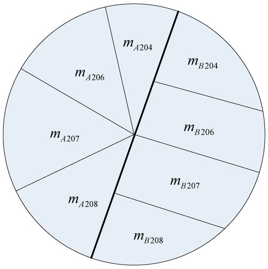
Figure 1.
Schematic diagram of lead quality composition structure of contamination point P.
On this basis, the contribution rates of contamination point P (, ) are defined as following three relationships, in detail:
Then the lead quality composition structures of the two pollution sources A and B are discussed. They are shown in Figure 2a,b.
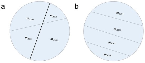
Figure 2.
Schematic diagram of lead fingerprint in lead pollution source A (a) and B (b).
According to the definition of lead fingerprint previously mentioned, the lead fingerprints of sources A, B, and contaminated point P can be measured by using MC-ICP-MS. Among them, the lead fingerprint of source A is , source B is , and contaminated point P is . The details are as follows:
In order to obtain the contribution rates of lead source A and B, according to equations 7–10, linear equations can be established for contaminated point P as follows:
There are a total of 12 equations in Equation (11), in which , , , , , , , , and are 10 unknown parameters. and are known parameters which can be obtained by experiments. Because Equation (11) is a set of linear equations, the number of unknown parameters is less than the number of equations (10 < 12), the equations can be solved. The calculated two lead pollution contribution rates are as follows:
So far, if there are two lead pollution sources, the contribution rates can be calculated based on the newly defined fingerprint by solving Equation (11). Therefore, we have successfully realized lead pollution sources’ identification. When the number of pollution sources increases, the following conclusions can be obtained by further discussion for Equation (11): With the increase in the number of lead pollution sources, the number of linear equations in Equation (11) also increases, but the increasing speed of the number of equations is less than the increasing speed of unknown parameters. When the number of lead pollution sources is 4, the number of linear equations is exactly equal to the number of unknown parameters. This is a critical point where we can resolve the lead pollution sources. When the number of lead sources is larger than 4, the number of linear equations is less than the number of unknown parameters. Therefore, as the number of lead sources is larger than 4, the system has infinite solutions according to the basic knowledge of linear algebra. The corresponding growth of the number of equations and the number of unknown parameters is shown in Table 3. Therefore, our proposed new analytic model could successfully address up to four lead pollution sources.
Table 3.
The possibilities of resolving the sources under condition of a plurality of lead pollution sources.
3.3. Validation of the Proposed New Analytic Model
To verify if our model could address the practical problems, we chose an industrial zone in the western region of the Guanzhong area, Shaanxi province, China, as the study area. The geographical environment of the study area is described below. In general, it is a narrow and long shape, and the terrain is high in the middle and low on both sides. The altitude difference is about 200 m, and the total area is about 20 km2. There are two reservoirs interconnected by a river in the northwest and southeast direction, respectively. The dominant wind direction is southeast wind and the secondary prevailing wind direction is north. The study area typically has a continental monsoon climate zone. The meteorological records show that the annual mean temperature is 11.2 °C, the average annual precipitation is 616.3 mm, and the average annual evaporation capacity is 1202.1 mm. The meteorological data collected in the past three years show that the mean wind speed is 2.19 m/s and the maximum wind speed is 19.0 m/s. A lead and zinc smelter and a thermal power plant are located in the region. In our study, we chose 32 sampling points in the soil. These 32 sampling points are distributed outside of the lead and zinc smelter in eight different directions (east, south, west, north, southeast, southwest, northeast, and northwest). Hence, there are four points in each direction. The distance between the point which is nearest to lead and zinc smelter and the wall is 500 m. The distribution regulation of the left three points in one direction is 1000 m, 1500 m, and 2000 m to the wall of the lead and zinc smelter, respectively. The study area and the 32 sampling points are shown in Figure 3 in detail. In addition, we have conducted several batches of sampling events for the raw ore of lead and zinc smelter, the raw coal of a coking plant and power plant, and the background value of this area. Average values of several replicates in each lead pollution sources are used. Additionally, the background value of the area is considered as a lead pollution source.
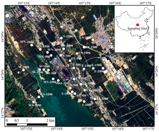
Figure 3.
The study area and distribution of the sampling points.
In our study, the content of heavy metal is analyzed by using Axios PW2200 (PANalytical B.V., Almelo, the Netherlands), and the Chinese first grade standard USS1-8 is used for experiment procedure controlling. The results show that the relative standard errors are all less than 10%. The lead isotope experiments are conducted in the State Key Laboratory of Loess and Quaternary Geology, Institute of Earth Environment, Chinese Academy of Sciences. Materials and methods for this assay were described in Section 2, and lead isotope ratios are measured by MC-ICP-MS. The experimental data error range is from 0.02% to 0.09%. The experimental results are shown in Table 4.
Table 4.
Lead isotope measurement results of the samples.
We chose raw coal of a coking plant, ore of lead and zinc smelter, raw coal of a power plant, and regional background value as four lead pollution resources. We then calculated the contribution rates of these four pollution sources based on the new analytical model. The calculation results are shown in Table 5.
Table 5.
Lead source analysis result basing on the new model.
It can be learned from Table 5 that the results of data points No. 14, No. 15, and No. 16 include negative values (−13.86%, −9.20%, −2.59%), which are possibly due to the interference from other lead pollution sources beyond our control. Specifically, after further study about these three points we realized that they are close to roads and villages. They are easily influenced by lead substances from automobile exhaust and burnt coal of households, the sources of which usually vary significantly. The other sites were not heavily influenced by such uncertain pollution sources. In addition, the new model is valid to the remaining 29 points. The analysis result shows the contribution rate of background value is stable and the average is 16.33%. The remaining three pollution sources have formed a complex effect on the study area, and their average contribution rates from large to small are as follows: Ore of smelting plant (35.28%), raw coal of coking plant (27.58%), and raw coal of power plant (20.81%). The contribution degree of each lead pollution source in the whole study area can be reflected based on the above sequence. Alongside this, the distribution characteristics of the contribution degree of each lead pollution source are slightly different when the direction and distance of the points are different. For example, in the south direction, the contribution rates of the lead and zinc smelter (23.75%, 28.33%, 27.81%, and 27.79%) are significantly less than the coking plant (i.e., 49.92%, 40.60%, 41.59%, and 39.00%).
4. Conclusions
This study reviews the previous studies on Pb pollution source identification, and then clarifies the concept of the lead fingerprints and builds a mathematical expression of lead fingerprints using the relative relationships of the four stable isotopes of lead. Based on lead fingerprints analysis, this study establishes a new pollution source analysis model and further discusses its application boundaries. Finally, a case study was conducted to verify this new model. We conclude that:
- (1)
- Gobeil’s model is incomplete and our new established pollution source identification model with lead fingerprints can overcome the limitations of Gobeil’s model to some extent.
- (2)
- When the number of the pollution sources is less than five, the lead contribution rates can be calculated accurately using our new model. It is not feasible to calculate lead contribution rates when the pollution sources are more than five. For example, in this study we found that the contribution rate from certain pollution sources is negative, because there is a significant interference from the other unknown pollution sources. Future research may include taking advantage of the other metal elements fingerprints to achieve more accurate calculations.
- (3)
- Moreover, our model can be applied to identify lead pollution sources in contaminated sites where lead compound pollutant enrichment occurs, and lead substances are transported under varying meteorological, terrain, and other conditions.
Supplementary Materials
The following are available online at https://www.mdpi.com/1660-4601/16/24/5059/s1, Figure S1: Schematic diagram of lead isotopic quality composition structure of sample.
Author Contributions
Data curation, T.F., C.-j.W., Y.L. and Z.L.; Formal analysis, T.F., C.-j.W., Y.L. and Z.L.; Funding acquisition, T.F.; Methodology, M.-m.F.; Writing—original draft, T.F.; Writing—review & editing, M.C., M.-m.F. and Z.L.
Funding
We greatly thank the Social Science Fund Project of Shaanxi Province (2017S001), the Natural Science Foundation Research Fund of Shaanxi Province (2018JM7003), and the Natural Science Foundation of China (Grant Nos. 71872141), and the talent fund of science and technology of Xi’an University of Architecture and Technology (RC1724) for their financial support.
Conflicts of Interest
The authors declare no conflict of interest.
References
- Needleman, H. Lead poisoning. Annu. Rev. Med. 2004, 55, 209–222. [Google Scholar] [CrossRef] [PubMed]
- Klaine, S.J.; Alvarez, P.J.J.; Batley, G.E. Nanomaterials in the environment: Behavior, fate, bioavailability, and effects. Environ. Toxicol. Chem. 2008, 27, 1825–1851. [Google Scholar] [CrossRef] [PubMed]
- Landmeyer, J.E.; Bradley, P.M.; Bullen, T.D. Stable lead isotopes reveal a natural source of high lead concentrations to gasoline-contaminated groundwater. Environ. Geol. 2003, 45, 12–22. [Google Scholar] [CrossRef]
- Lantzy, R.J.; Mackenzie, F.T. Atmospheric trace metals: Global cycles and assessment of man’s impact. Geochim. Cosmochim. Acta 1979, 43, 511–525. [Google Scholar] [CrossRef]
- Gobeil, C.; Johnson, W.K.; Macdonald, R.W. Sources and burden of lead in St. Lawrence estuary sediments: Isotopic evidence. Environ. Sci. Technol. 1995, 29, 193–201. [Google Scholar] [PubMed]
- Woodhead, J.D.; Hergt, J.M. Application of the ‘double spike’ technique to Pb-isotope geochronology. Chem. Geol. 1997, 138, 311–321. [Google Scholar] [CrossRef]
- Weaver, V.M.; Davoli, C.T.; Heller, P.J. Benzene exposure, assessed by urinary trans, trans-muconic acid, in urban children with elevated blood lead levels. Environ. Health Perspect. 1996, 104, 318–323. [Google Scholar] [CrossRef]
- Shiel, A.E.; Weis, D.; Orians, K.J. Evaluation of zinc, cadmium and lead isotope fractionation during smelting and refining. Sci. Total Environ. 2010, 408, 2357–2368. [Google Scholar] [CrossRef]
- Cheng, H.; Hu, Y. Lead (Pb) isotopic fingerprinting and its applications in lead pollution studies in China: A review. Environ. Pollut. 2010, 158, 1134–1146. [Google Scholar] [CrossRef]
- Choi, M.S.; Yi, H.I.; Ye, S. Identification of Pb sources in Yellow Sea sediments using stable Pb isotope ratios. Mar. Chem. 2007, 107, 255–274. [Google Scholar] [CrossRef]
- Finkelstein, M.E.; Kuspa, Z.E.; Welch, A. Linking cases of illegal shootings of the endangered California condor using stable lead isotope analysis. Environ. Res. 2014, 134, 270–279. [Google Scholar] [CrossRef] [PubMed]
- Tornos, F.; Arias, D. Sulfur and lead isotope geochemistry of the Rubiales Zn–Pb ore deposit (NW Spain). Eur. J. Mineral. 1993, 5, 763–773. [Google Scholar] [CrossRef]
- Marcantonio, F.; Zimmerman, A.; Xu, Y. A Pb isotope record of mid-Atlantic US atmospheric Pb emissions in Chesapeake Bay sediments. Mar. Chem. 2002, 77, 123–132. [Google Scholar] [CrossRef]
- Rio-Salas, R.D.; Ruiz, J.; O-Villanueva, M.D.L. Tracing geogenic and anthropogenic sources in urban dusts: Insights from lead isotopes. Atmos. Environ. 2012, 60, 202–210. [Google Scholar] [CrossRef]
- Tsuji, L.J.S.; Wainman, B.C.; Martin, I.D. The identification of lead ammunition as a source of lead exposure in First Nations: The use of lead isotope ratios. Sci. Total Environ. 2008, 393, 291–298. [Google Scholar] [CrossRef] [PubMed]
- Eades, L.J.; Farmer, J.G.; Mackenzie, A.B. Stable lead isotopic characterisation of the historical record of environmental lead contamination in dated freshwater lake sediment cores from northern and central Scotland. Sci. Total Environ. 2002, 292, 55–67. [Google Scholar] [CrossRef]
- Bird, G.; Brewer, P.A.; Macklin, M.G. Quantifying sediment-associated metal dispersal using Pb isotopes: Application of binary and multivariate mixing models at the catchment-scale. Environ. Pollut. 2010, 158, 2158–2169. [Google Scholar] [CrossRef] [PubMed]
- Bird, G.; Brewer, P.A.; Macklin, M.G. Pb isotope evidence for contaminant-metal dispersal in an international river system: The lower Danube catchment, Eastern Europe. Appl. Geochem. 2010, 25, 1070–1084. [Google Scholar] [CrossRef]
- Bird, G. Provenancing anthropogenic Pb within the fluvial environment: Developments and challenges in the use of Pb isotopes. Environ. Int. 2011, 37, 802–819. [Google Scholar] [CrossRef]
- Dumas, C.; Aubert, D.; Durrieu, D.M.X. Storm-induced transfer of particulate trace metals to the deep-sea in the Gulf of Lion (NW Mediterranean Sea). Environ. Geochem. Health 2014, 36, 995–1014. [Google Scholar] [CrossRef]
- Miller, J.R.; Lechler, P.J.; Mackin, G. Evaluation of particle dispersal from mining and milling operations using lead isotopic fingerprinting techniques, Rio Pilcomayo Basin, Bolivia. Sci. Total Environ. 2007, 384, 355–373. [Google Scholar] [CrossRef] [PubMed]
- Chiaradia, M.; Chenhall, B.E.; Depers, A.M. Identification of historical lead sources in roof dusts and recent lake sediments from an industrialized area: Indications from lead isotopes. Sci. Total Environ. 1997, 205, 107–128. [Google Scholar] [CrossRef]
- Chiaradia, M.; Cupelin, F. Behaviour of airborne lead and temporal variations of its source effects in Geneva (Switzerland): Comparison of anthropogenic versus natural processes-a descriptive analysis of organic and elemental carbon concentrations. Atmos. Environ. 2000, 34, 959–971. [Google Scholar] [CrossRef]
- Camarero, L.; Masqué, P.; Devos, W.; Ani-Ragolta, I. Historical Variations in Lead Fluxes in the Pyrenees (Northeast Spain) from a Dated Lake Sediment Core. Water Air Soil Pollut. 1988, 105, 439–449. [Google Scholar] [CrossRef]
- Álvarez-Iglesias, P. Isotopic identification of natural vs. anthropogenic lead sources in marine sediments from the inner Ría de Vigo. Sci. Total Environ. 2012, 437, 22–35. [Google Scholar] [CrossRef]
- Luo, X.S.; Yan, X.; Wang, Y.L. Source identification and apportionment of heavy metals in urban soil profiles. Chemosphere 2015, 127, 152–157. [Google Scholar] [CrossRef]
- Kylander, M.E.; Spiro, B.; Weiss, D.J. Refining the pre-industrial atmospheric Pb isotope evolution curve in Europe using an 8000 year old peat core from NW Spain. Earth. Planet. Sci. Lett. 2005, 240, 467–485. [Google Scholar] [CrossRef]
- Lima, A.L.; Bergquist, B.A.; Boyle, E.A. High-resolution historical records from Pettaquamscutt River basin sediments: 2. Pb isotopes reveal a potential new stratigraphic marker. Geochim. Cosmochim. Acta 2005, 69, 1813–1824. [Google Scholar] [CrossRef]
- Anderson, B.; Gemmell, J.; Nelson, D. Lead isotope evolution of mineral deposits in the Proterozoic Throssell group, Western Australia. Econ. Geol. 2002, 97, 897–911. [Google Scholar] [CrossRef]
- Cao, S.; Duan, X.; Zhao, X. Isotopic ratio based source apportionment of children’s blood lead around coking plant area. Environ. Int. 2014, 73, 158–166. [Google Scholar] [CrossRef]
- Cao, S.; Duan, X.; Zhao, X. Levels and source apportionment of children’s lead exposure: Could urinary lead be used to identify the levels and sources of children’s lead pollution? Environ. Pollut. 2015, 199, 18–25. [Google Scholar] [CrossRef] [PubMed]
- Zhao, D.Y.; Wei, Y.M. Applications of lead isotope ratios for identification and apportionment on pollution sources in food. J. Nucl. Agric. Sci. 2011, 25, 534–539. [Google Scholar]
© 2019 by the authors. Licensee MDPI, Basel, Switzerland. This article is an open access article distributed under the terms and conditions of the Creative Commons Attribution (CC BY) license (http://creativecommons.org/licenses/by/4.0/).