Abstract
Hypertension (HT) is an extreme increment in blood pressure that can prompt a stroke, kidney disease, and heart attack. HT does not show any symptoms at the early stage, but can lead to various cardiovascular diseases. Hence, it is essential to identify it at the beginning stages. It is tedious to analyze electrocardiogram (ECG) signals visually due to their low amplitude and small bandwidth. Hence, to avoid possible human errors in the diagnosis of HT patients, an automated ECG-based system is developed. This paper proposes the computerized segregation of low-risk hypertension (LRHT) and high-risk hypertension (HRHT) using ECG signals with an optimal orthogonal wavelet filter bank (OWFB) system. The HRHT class is comprised of patients with myocardial infarction, stroke, and syncope ECG signals. The ECG-data are acquired from physionet’s smart health for accessing risk via ECG event (SHAREE) database, which contains recordings of a total 139 subjects. First, ECG signals are segmented into epochs of 5 min. The segmented epochs are then decomposed into six wavelet sub-bands (WSBs) using OWFB. We extract the signal fractional dimension (SFD) and log-energy (LOGE) features from all six WSBs. Using Student’s t-test ranking, we choose the high ranked WSBs of LOGE and SFD features. We develop a novel hypertension diagnosis index (HDI) using two features (SFD and LOGE) to discriminate LRHT and HRHT classes using a single numeric value. The performance of our developed system is found to be encouraging, and we believe that it can be employed in intensive care units to monitor the abrupt rise in blood pressure while screening the ECG signals, provided this is tested with an extensive independent database.
1. Introduction
High blood pressure or hypertension (HT) is a severe disease, and patients have no symptoms in the early stages. Due to low awareness and without proper treatment, this may result in it being more harmful for hypertensive patients and increases the possibility of having cardiovascular diseases. In today’s world, due to hypertension, the number of deaths has increased [1]. As per the 2005 global data, in India, 20.6% of males and 20.9% of females were suffering from hypertension. This trend is expected to rise to 22.9% (male) and 23.6 (female)%. The current survey shows the pervasiveness of hypertension in rural and urban India to be 25% and 10%, respectively. Only 25% of hypertension patients have their blood pressure (BP) under control after the treatment [2]. The BP is the pressure exerted by the blood against the walls of the arteries. The pressure relies on the work being done by the heart and the obstruction of the blood vessels [2]. The possible reasons for hypertension are less physical activity, lifestyle, smoking, stress, family history, and kidney disease [1]. Hence, it is a crucial issue to develop awareness, medical care, and treatment for hypertension. Clinically, we can classify hypertension into mild, moderate, and severe states [3]. It is more important to identify the severity of hypertension. The ranges of normal and hypertension blood pressure are given in Table 1.

Table 1.
Typical blood pressure ranges [3].
The electrocardiogram (ECG) is a valuable tool used to measure the electrical activity of the heart [4,5,6,7,8,9]. Currently, there are various wearable and non-intrusive devices used to monitor hypertension using ECG [10,11,12]. To diagnose hypertension in a clinical environment, blood pressure measurement, which is the gold standard, is used. Depending on the range of blood pressure values (Table 1), the patients are classified as low-risk hypertension (LRHT) and high-risk hypertension (HRHT) patients.
Various techniques, algorithms, applications, and devices have been developed to detect and monitor hypertensive patients. Voss et al. [13] used high-resolution ECG, heart rate variability (HRV), blood pressure variability (BPV), and baroreflex sensitivity (BRS) signals. They found a difference in HRV signals of a normal pregnant female and a hypertensive pregnant female.
Poddar et al. [14] used the automated classification of hypertension and coronary artery disease patients using the probabilistic neural network (PNN), k-nearest neighbor (KNN), and support vector machine (SVM) classifiers with HRV analysis. They obtained the highest classification accuracy of 96.67%. Natrajan et al. [15] observed a significant reduction in high-frequency and an increase in low-frequency HRV signals of hypertensive patients.
Melillo and Izzo [16] used HRV signals along with various machine learning algorithm (SVM, decision tree (DT), and convolution neural network (CNN)) to identify HRHT patients, and obtained the highest accuracy of 87.8%.
Recently, Ni and Wang used fine-grained HRV-based methods and obtained an accuracy of 95% [3]. Song et al. [17] classified normal, hypertensive, and coronary heart disease (CHD) patients using HRV signals and the naive Bayes classifier. They obtained 92.3% classification accuracy.
Yue et al. [18] used machine learning algorithms to implement an automatic risk indication for mask-hypertension using HRV analysis [18]. They found that HRV, parameters in essential hypertension (EH), and mask hypertension (MH) in patients have significantly decreased.
Ni et al. [10] studied hypertension patients and normal subjects using a three-dimensional feature method with continuous HRV monitoring. They obtained the highest classification accuracy of 93.33% [10]. Mussalo et al. [19] analyzed different HRV features for various stages of hypertension patients. They observed significant changes in the HRV parameters of hypertension patients.
Thus, all the above-mentioned studies used HRV signals derived from ECG. The novelty of the proposed work is that we use optimal wavelet-based features extracted from ECG signals instead of using HRV. The optimal orthogonal wavelets that are designed by optimizing spectral localization (SL) were used in the proposed study [20]. Wavelets are regarded as the best tools for the analysis of non-stationary signals, including ECG [21,22,23,24]. Hence, we employed wavelet-based ECG features to develop an automated system for the identification of LRHT and HRHT. We applied the SL-optimized wavelet filter due to the following reasons [25]: (i) In conventional methods, most of the studies were performed by optimizing stop-band and pass-band energies by accurately defining the edge frequencies [26]. That may not be understood a priori in each application. Here, we used the orthogonal wavelet filter [27,28,29] designed by minimizing its frequency spread. (ii) Minimizing the spectral localization of a filter, it is possible to take care of both ripples and the transition band of the filter. (iii) The SL optimized filter gives precisely fewer ripples and sharp roll-off [30].
In our study, we used the SL optimal OWFB. Using a semi-definite program (SDP) technique [31,32], we optimized the filter coefficients, and the interior point algorithm provided the optimized solutions [33,34,35]. Hence, we tested the optimized OWFBs for analyzing ECG signals in order to separate LRHT from HRHT patients. The OWFB provided various sub-bands (SBs) of the ECG signal, and from these SBS, we extracted log energy (LOGE) and spectral fractal dimension (SFD) features [36]. Student’s t-test ranking was applied to all extracted features and the most significant SBs of SFD and LOGE features.
The main contribution of this study is the development of the hypertension diagnosis index (HDI) using OWFB-based SFD and LOGE features. HDI provides the discrimination of LRHT and HRHT by a single numeric value. In a clinical environment, HDI is simpler and easier to use for the diagnosis of disease.
The remainder of the paper is arranged in the following manner. We discuss the details of the ECG dataset in Section 2. The methodology and an optimally-designed OWFB are described in Section 3. Section 4 illustrates the results obtained. In Section 5, we discuss the results obtained. At last, the concluding remarks of the paper are outlined in Section 6.
2. Dataset
The dataset for this study was taken from physionet’s smart health for assessing the risk of events of ECG signals (SHAREE project) https://archive.physionet.org/pn6/shareedb/. A total of 139 subjects’ ECG recordings were used with a length of 2 h:10 min:12 s, approximately, for each ECG signal. Each ECG recording contained three rows (channels/ signals) III, V3, and V5, and each signal had 1 million samples, approximately. In our study, leads III, V3, and V5 were named CH1 (Channel 1), CH2, and CH3, respectively. The ECG sampling frequency was 128 Hz with an 8-bit resolution, and the sampling interval was 0.0078125 s. The average age of patients was 71.4 for LRHT and 74.5 years for HRHT, which included 49 female and 90 male patients. To detect major cardiovascular and cerebrovascular events, patients were observed for a year. Seventeen patients (three syncopal, three strokes, eleven myocardial infarctions) were identified as HRHT subjects, while 122 patients as LRHT subjects. The dataset was authorized by the Federico II University Hospital Trust’s Ethics Committee. All subjects involved in data collection provided consent and signed for the experimental use of data. Table 2 gives the details and statistics of the patients included in gathering the SHAREE database. We segmented our ECG signal into 5-min signals. After the segmentation of ECG signals, we obtained 3172 ECG epochs corresponding to LRHT and 442 epochs for HRHT subjects for each channel. Figure 1, Figure 2, Figure 3 and Figure 4 show the LRHT and HRHT ECG signals of 5 min.
Table 2.
Statistics of the patients employed in acquiring the database. LRHT, low-risk hypertension; HRHT, high-risk hypertension.
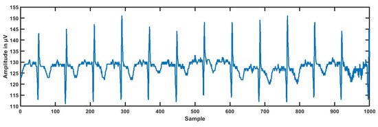
Figure 1.
Typical low-risk hypertension (LRHT) ECG signal.
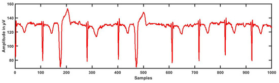
Figure 2.
Typical high-risk hypertension (HRHT) myocardial infraction ECG signal.
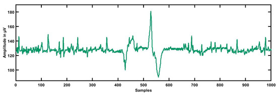
Figure 3.
Typical high-risk hypertension (HRHT) syncope ECG signal.
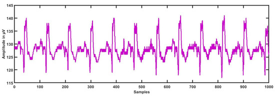
Figure 4.
Typical high-risk hypertension (HRHT) stroke ECG signal.
3. Methodology
To separate LRHT and HRHT automatically, the optimally-designed OWFB was used. A total of six sub-bands (SBs) were produced using wavelet decomposition [26]. Five SBs were used for detail, and one SB for approximation was used for ECG signals. After the wavelet decomposition into six SBs’ log energy (LOGE) and signal fractional dimensions (SFD), features were extracted from all SBs. Thus, a total of 12 features were obtained from each ECG epoch, six LOGE and six SFD. The novelty of this work is the development of the HDI, which can be used to discriminate LRHT and HRHT ECG signals. The detailed outline of the proposed automated high-risk hypertension detection system is shown in Figure 5.
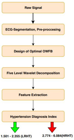
Figure 5.
Workflow of the proposed work. OWFB, optimal orthogonal wavelet filter bank.
3.1. ECG Segmentation
For fast computing, we pre-processed the ECG signals. Long duration (2 h:10 min:12 s) ECG data were segmented for the 5-min duration, then each ECG segment was normalized using the Z-score before applying to the wavelet filter bank.
3.2. Design of Filter Bank
The OWFB contained two sets of filter banks (FLBs) (Figure 6); one was called synthesis FLB, and another one was analysis FLB [25]. Both FLBs contained low-pass (LP) and high-pass (HP) filters. For analysis FLB, the outputs of LP and HP were downsampled by 2, and in synthesis FLB, the inputs to HP and LP were up-sampled by a factor of 2 prior to applying them. Let and be the LP and HP filters, respectively, for analysis FLB. Let and be the LP and HP filters of synthesis FLB, as shown in Figure 6. The analysis and synthesis LP filters were time-reversed copies of each other, which is an important characteristic of OWFB [20]. Using the quadrature conjugation technique [37], the HP filters and can be derived from LP filters and . Hence, we can get the remaining three filters directly from the LP analysis filter . The perfect reconstruction (PR) and zero-moment (ZM) constraints [28] must be obeyed by optimal OWFB for output to be a delayed replica of the input [29].
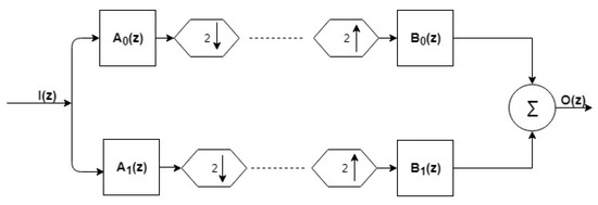
Figure 6.
Two-channel OWFB.
For perfect reconstruction, the filter must fulfill the orthogonality condition as mentioned below [25]:
Let , be called the product filter [34]. We can rewrite (1) in terms of the product filter as below:
Let be the frequency response of the product filter, which is represented by [34]:
Now, we can represent the perfect reconstruction condition (2) in the frequency domain as,
For the real , [38]. Here, to design a real-coefficient orthogonal wavelet filter bank, a positive value of the for is needed. The total number of roots at can be defined as zero moments (ZM) of the filter [29,39]. To design the LP filter with -order, ZMs there should be zeros at in the product filter.
If the product filter satisfies Equation (2) and the , condition, we can convert the designed OWFB into the designed product filter [40,41,42]. After designing , we can obtain the required analysis LP filter using spectral factorization [35,43].
Constraint in the Time-Domain and Objective Function
To design the optimal OWFB, consider a(n) to be the unit impulse response of finite impulse response analysis LP filter of and b(n) be the unit impulse response of synthesis LP filter of order . The optimality criterion to design the orthogonal filter design is to minimize the mean squared spectral localization (MSSL). MSSL happens to be the same for both analysis and synthesis filters as the former is the time-reversed replica of the latter [24,32,44].
Now, we can define the MSSL, of the filter as [45]:
where E represents the squared-norm or energy of the filter. Imposing M zero-moments (regularity) and orthogonality constraints, we design an optimal OWFB with the objective of having minimum MSSL. The optimization problem for the filter design can be mentioned as below.
Hence, to minimize MSSL (6a) for the given regularity (6c) and orthogonality (6b) constraints, a constrained optimization problem was formulated. To develop a convex formulation, we need to express the constraints and objective function in terms of . As specified above, the sequence (impulse response of the ) is an auto-correlation sequence whose spectrum satisfies the non-negativity condition . We can write the objective function (5) in the form of the product filter as:
Thus, the optimization problem (6) can be represented in the form of the product filter as mentioned below:
The above-mentioned optimization problem (8) is a non-convex optimization problem in variable , whereas the optimization problem in (6) is a convex optimization problem in variable . Now, we intend to convert the non-convex problem into a convex problem to get an optimal solution. Using (8b), the half-band condition is linear in variable . Equations (8c) and (8d) represent the regularity conditions, which are also linear constraints. Only the non-positivity condition (8e) is a non-linear semi-infinite constraint (one constraint each for every ), which needs to be converted into a finite constraint to formulate the convex optimization problem. Sharma and Moulin et al. [46,47] used the discretization method to transform the semi-infinite constraint into finite constraints. However, due to the inaccurate solution obtained by the discretization method, it is not advisable to use it.
Hence, we used the Kalman–Yakubovich–Popov lemma (KYPL) [48] for the formulation of a semidefinite program (SDP). By the KYP lemma, (8e) exists only if there exists a symmetric positive such that:
Hence, the objective function (8a) in terms of sequence p(n) can be given below:
Here, is and is . Using (10), we obtained the objective function as a linear function of . Furthermore, all constraints can be expressed as a linear function of . Hence, the optimization problem (8) can be written as the following convex optimization problem [25].
Now, our optimization problem is convex as the objective function, and all the constraints are convex. To find the global solution of the problem, we can use interior point algorithms such as SedDumiand SPDT3 [49].The tools SPDT3 and SedDumi can solve the optimization problem accurately and efficiently. After finding the optimal , the next step is to obtain the desired low-pass filter using spectral localization of .
3.3. Wavelet Decomposition
We designed optimal WFBs for sub-band decomposition of ECG signals [50,51]. We employed five levels of decomposition. The five-level wavelet decomposition gave us precise information about the 6 SBs of each ECG epoch. By this technique, we have extracted the desired frequencies present in the ECG signal. Hence, the five-level wavelet decomposition of the ECG signal was done by this method. The six SBs had five detailed (SB1–SB5) and one approximate (SB6) SBs.
3.4. Features Used
The selection of essential features was an important part of this work. Using this method, we were able to classify LRHT and HRHT ECG signals. The log energy (LOGE) and signal fractal dimension (SFD) features were computed from all six SBs.
Log energy (LOGE): To calculate the LOGE of each SB of the ECG signal, the logarithm of energy needs to be computed. The general formula of the log energy is [25]:
where is the log energy of the sub-band and is the amplitude of the sample of the sub-band.
Signal fractal dimension (SFD): Fractals are figures of geometry or curves that are a subset of a Euclidean space. These curves have the Hausdorff dimension strictly exceeding the topological dimension. The fractal dimension provides a statistical magnitude to the complexity detailing the pattern or fractal pattern with respect to the scale with which it is measured [25].
We can write the SFD equation as below:
where is the number of self-similar patterns used to fill the original pattern and m is the ratio used to decompose the original pattern into self-similar patterns.
3.5. Hypertension Diagnosis Index
The extracted highly-significant features in Table 3 were used to develop the mathematical model (14) to discriminate the two classes [52,53,54].
Table 3.
Mean and standard deviation for CH3.
We propose a hypertension diagnosis index (HDI) to discriminate against the LRHT and HRHT by a single numeric value. We used two sets of features (SFD and LOGE) with the highest t-value (lowest p-value) to compute the HDI [55]. We formed the mathematical simulation given by:
where and represent LOGE features extracted from SB2 and SB3, while , , , and represent the SFD feature extracted from SB6, SB2, SB3, and SB4.
4. Results
Using the 5-min ECG dataset, it is segmented in 3172 epochs of low-risk hypertension and 442 epochs of high-risk hypertension. Our whole experimental work was performed using MATLAB Version 9.1 with an Intel Xeon 3.5 gigahertz (GHz) and 16 gigabytes (GB) of random access memory (RAM). Table 3, Table 4 and Table 5 represent the statistical differences of LRHT and HRHT for the CH3, CH1, and CH2 ECG signals.
Table 4.
Mean and standard deviation for CH1. SB, sub-band.
Table 5.
Mean and standard deviation for CH2.
The result of Student’s t-test for each SB is shown in Table 6 with t-values and p-values for both features (SFD and LOGE). Table 7 shows the result of the calculated HDI. Table 7 presents the range of HDI and shows a significant difference in the LRHT and HRHT. Figure 7 shows the discrimination between LRHT and HRHT by the significant numeric value. The segregation of both classes by HDI is more simple and easy to use in a clinical environment.
Table 6.
Student’s t-test results, t-value and p-value. SFD, signal fractional dimension; LOGE, log-energy.
Table 7.
Hypertension diagnosis index (HDI) range for the LRHT and HRHT classes.
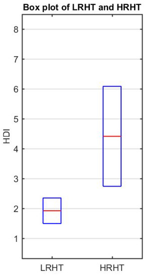
Figure 7.
Box plot of LRHT and HRHT.
5. Discussion
The aim of this study was to calculate the performance of features (LOGE and SFD) extracted from novel optimal OWFB. In this research work, using spectrum-localized OWFB-based non-linear features, we could identify HRHT patients using a single numeric value. The employed optimal OWFB-based features yielded 100% discrimination of LRHT and HRHT patients using HDI. The salient features of our developed automated system are given below:
- From Table 3, LOGE values of SB2–SB6 showed significant changes corresponding to LRHT and HRHT patients.
- SFD of SB2 for LRHT and HRHT obtained the highest mean value, while SB1 showed the lowest mean value. LOGE of SB1 yielded the highest mean value for LRHT, and SB2 for HRHT patients yielded the lowest mean value.
- The novelty of the proposed work was the development of HDI to discriminate between the two classes using a single value.
- Table 7 presents the range of HDI and shows a significant difference in the LRHT and HRHT by a numeric value.
- We did not need classifiers, which involve training and testing. It was fast and involved only the extraction of two feature sets.
- The spectral localization technique was used to analyze non-stationary characteristics of the ECG signal. As we used spectral localized OWFB, our proposed work was unique as compared to other research works [3,16].
- For better and fast computation, we used fewer features. The length of the ECG signal was 5 min. Hence, it was not computationally intensive and quicker in diagnosis.
- Using the same database, Melillo and Izzo used various machine learning algorithms (SVM, decision tree (DT), and convolution neural network (CNN)) and obtained the highest accuracy of 87.8% with HRV signals [16]. Recently, Ni and Wang [3] obtained an accuracy of 95% using heart rate variability (HRV) signals.
- Many studies have used HRV-based techniques to detect hypertension; we used wavelet-based features directly extracted from ECG. Our method was different from HRV-based methods and easy to use in the clinical environment [3].
- The performance of the system was found to be promising, and we expect that it can be employed in intensive care units to monitor the abrupt rise in blood pressure while screening the ECG signals, provided it is tested with an extensive independent database.
- The present research work was conducted using 139 ECG recordings segmented into 3614 (3172 as LRHT, 442 as HRHT (78 stroke, 78 syncope, and 286 myocardial infarction)) epochs of 5 min each comprised of CH1, CH2, and CH3. The ECG dataset was obtained from https://archive.physionet.org/pn6/shareedb/. Our whole experimental work was performed using MATLAB. Table 7 shows the results of the automated detection of LRHT and HRHT classes. In Table 8, we compare our proposed work with other methods. Using HDI, we can discriminate between the two classes by just the single numeric value with 100% accuracy.
Table 8. Comparison of work done for automated detection of hypertension ECG signals. HRV, heart rate variability.
The dataset consisted of 3614 ECG epochs, out of which 87% were LRHT and 13% were HRHT ECG signals. This imbalanced dataset is one of the limitations of our work. In general, LRHT data are greater than HRHT data. To reduce this imbalance problem, synthetic balancing data are needed. The other limitation of our research work is the selection of the optimal number of ZMs and the length of the filter. In order to achieve accurate identification of HRHT, we cannot predict the estimated order and ZM a priori.
In recent studies, deep learning methods were widely used for classification problems [56,57,58,59]. We can use deep learning methods like convolution neural networks (CNN) [60]. In deep learning-based techniques, we need not extract, select, and classify the handcrafted features. However, due to extensive data processing, the computational complexity is enormous. Hence, they require fast processing workstations and graphics processing units (GPU).
6. Conclusions
In this study, we used optimal OWFB-based non-linear features to discriminate LRHT and HRHT ECG signals automatically using an index (HDI). The five-level wavelet decomposition of ECG signals using optimal OWFB produced six (SBs). The LOGE and SFD features were extracted for all six SBs. Our proposed OWFB-based method was adequate to discriminate the HT ECG signals accurately utilizing features (LOGE and SFD) by a single numeric value. To evaluate the performance of the optimal wavelet filter bank, HDI was developed, which separated LRHT and HRHT groups using the proposed index. Our results show that the developed model was better than the other existing systems and ready to be tested using a large database. In the future, we plan to test the performance of our technique to detect the severity of hypertension using certain machine learning-based techniques with the same database. We also intend to use deep learning-based methods for the classification of LRHT and HRHT ECG signals as our future work.
Author Contributions
Conceptualization, M.S. and U.R.A.; methodology, J.S.R.; software, J.S.R.; validation, M.S., U.R.A. and J.S.R.; formal analysis, M.S. and U.R.A.; investigation, J.S.R.; resources, M.S. and U.R.A.; data curation, U.R.A.; writing—original draft preparation, J.S.R.; writing—review and editing, M.S. and U.R.A.; visualization, M.S.; supervision, M.S. and U.R.A.; project administration, M.S. and U.R.A.
Funding
This research received no external funding.
Conflicts of Interest
The authors declare no conflict of interest.
References
- WHO. A Global Brief on Hypertension; WHO/DCO/WHD/2013.2; WHO: Geneva, Switzerland, 2013; pp. 1–40. [Google Scholar]
- Kearney, P.M.; Whelton, M.; Reynolds, K.; Muntner, P.; Whelton, P.K.; He, J. Global burden of hypertension: Analysis of worldwide data. Lancet 2005, 365, 217–223. [Google Scholar] [CrossRef]
- Ni, H.; Wang, Y.; Xu, G.; Shao, Z.; Zhang, W.; Zhou, X. Multiscale Fine-Grained Heart Rate Variability Analysis for Recognizing the Severity of Hypertension. Comput. Math. Methods Med. 2019, 2019, 1–9. [Google Scholar] [CrossRef] [PubMed]
- Sharma, M.; Singh, S.; Kumar, A.; Tan, R.S.; Acharya, U.R. Automated detection of shockable and non-shockable arrhythmia using novel wavelet-based ECG features. Comput. Biol. Med. 2019, 103446. [Google Scholar] [CrossRef] [PubMed]
- Sharma, M.; Acharya, U.R. A new method to identify coronary artery disease with ECG signals and time-Frequency concentrated antisymmetric biorthogonal wavelet filter bank. Pattern Recognit. Lett. 2019, 125, 235–240. [Google Scholar] [CrossRef]
- Sharma, M.; Tan, R.S.; Acharya, U.R. Detection of shockable ventricular arrhythmia using optimal orthogonal wavelet filters. Neural Comput. Appl. 2019. [Google Scholar] [CrossRef]
- Sharma, M.; Tan, R.S.; Acharya, U.R. Automated heartbeat classification and detection of arrhythmia using optimal orthogonal wavelet filters. Inform. Med. Unlocked 2019, 100221. [Google Scholar] [CrossRef]
- Bhurane, A.A.; Sharma, M.; San-Tan, R.; Acharya, U.R. An efficient detection of congestive heart failure using frequency localized filter banks for the diagnosis with ECG signals. Cogn. Syst. Res. 2019. [Google Scholar] [CrossRef]
- Faust, O.; Acharya, R.; Krishnan, S.; Min, L.C. Analysis of cardiac signals using spatial filling index and time-frequency domain. Biomed. Eng. Online 2004, 3, 30. [Google Scholar] [CrossRef]
- Ni, H.; Cho, S.; Mankoff, J.; Yang, J.; Dey, A.k. Automated recognition of hypertension through overnight continuous HRV monitoring. J. Ambient. Intell. Humaniz. Comput. 2018, 9, 2011–2023. [Google Scholar] [CrossRef]
- Kwon, S.; Kang, S.; Lee, Y.; Yoo, C.; Park, K. Unobtrusive monitoring of ECG-derived features during daily smartphone use. In Proceedings of the 2014 36th Annual International Conference of the IEEE Engineering in Medicine and Biology Society, Chicago, IL, USA, 26–30 August 2014; pp. 4964–4967. [Google Scholar] [CrossRef]
- Ji Lee, H.; Hwang, S.; Yoon, H.; Kyu Lee, W.; Park, K. Heart Rate Variability Monitoring during Sleep Based on Capacitively Coupled Textile Electrodes on a Bed. Sensors 2015, 15, 11295–11311. [Google Scholar] [CrossRef]
- Voss, A.; Baumert, M.; Baier, V.; Stepan, H.; Walther, T.; Faber, R. Autonomic Cardiovascular Control in Pregnancies With Abnormal Uterine Perfusion. Am. J. Hypertens. 2006, 19, 306–312. [Google Scholar] [CrossRef] [PubMed]
- Poddar, M.; Birajdar, A.C.; Virmani, J. Kriti. Chapter 5—Automated Classification of Hypertension and Coronary Artery Disease Patients by PNN, KNN, and SVM Classifiers Using HRV Analysis; Academic Press: Cambridge, MA, USA, 2019; pp. 99–125. [Google Scholar] [CrossRef]
- Natarajan, N.; Balakrishnan, A.K.; Ukkirapandian, K. A study on analysis of Heart Rate Variability in hypertensive individuals. Int. J. Biomed. Adv. Res. 2014, 5, 109–111. [Google Scholar] [CrossRef]
- Melillo, P.; Izzo, R.; Orrico, A.; Scala, P.; Attanasio, M.; Mirra, M.; Luca, N.; Pecchia, L. Automatic Prediction of Cardiovascular and Cerebrovascular Events Using HRV Analysis. PLoS ONE 2015, 10, e0118504. [Google Scholar] [CrossRef] [PubMed]
- Song, Y.; Ni, H.; Zhou, X.; Zhao, W.; Wang, T. Extracting Features for Cardiovascular Disease Classification Based on Ballistocardiography. In Proceedings of the 2015 IEEE 12th Intl Conf on Ubiquitous Intelligence and Computing and 2015 IEEE 12th Intl Conf on Autonomic and Trusted Computing and 2015 IEEE 15th Intl Conf on Scalable Computing and Communications and Its Associated Workshops (UIC-ATC-ScalCom), Beijing, China, 10–14 August 2015; pp. 1230–1235. [Google Scholar] [CrossRef]
- Yue, W.w.; Yin, J.; Chen, B.; Zhang, X.; Wang, G.; Li, H.; Chen, H.; Jia, R.y. Analysis of Heart Rate Variability in Masked Hypertension. Cell Biochem. Biophys. 2014, 70, 201–204. [Google Scholar] [CrossRef]
- Mussalo, H.; Vanninen, E.; Ikaheimo, R.; Laitinen, T.; Laakso, M.; Lansimies, E.; Hartikainen, J. Heart rate variability and its determinants in patients with severe or mild essential hypertension. Clin. Physiol. 2001, 21, 594–604. [Google Scholar] [CrossRef]
- Sharma, M.; Bhurane, A.A.; Acharya, U.R. MMSFL-OWFB: A novel class of orthogonal wavelet filters for epileptic seizure detection. Knowl. Based Syst. 2018, 160, 265–277. [Google Scholar] [CrossRef]
- Sharma, M.; Tan, R.S.; Acharya, U.R. A novel automated diagnostic system for classification of myocardial infarction ECG signals using an optimal biorthogonal filter bank. Comput. Biol. Med. 2018. [Google Scholar] [CrossRef]
- Zala, J.; Sharma, M.; Bhalerao, R. Tunable Q - wavelet transform based features for automated screening of knee-joint vibroarthrographic signals. In Proceedings of the 2018 International Conference on Signal Processing and Integrated Networks (SPIN), Noida, India, 22–23 February 2018. [Google Scholar]
- Sharma, M.; Agarwal, S.; Acharya, U.R. Application of an optimal class of antisymmetric wavelet filter banks for obstructive sleep apnea diagnosis using ECG signals. Comput. Biol. Med. 2018, 100, 100–113. [Google Scholar] [CrossRef]
- Sharma, M.; Dhere, A.; Pachori, R.B.; Acharya, U.R. An automatic detection of focal EEG signals using new class of time–frequency localized orthogonal wavelet filter banks. Knowl.-Based Syst. 2017, 118, 217–227. [Google Scholar] [CrossRef]
- Sharma, M.; Raval, M.; Acharya, U.R. A new approach to identify obstructive sleep apnea using an optimal orthogonal wavelet filter bank with ECG signals. Informatics Med. Unlocked 2019, 16, 100170. [Google Scholar] [CrossRef]
- Sharma, M.; Dhere, A.; Pachori, R.B.; Gadre, V.M. Optimal duration-bandwidth localized antisymmetric biorthogonal wavelet filters. Signal Process. 2017, 134, 87–99. [Google Scholar] [CrossRef]
- Sharma, M.; Acharya, U.R. Analysis of knee-joint vibroarthographic signals using bandwidth-duration localized three-channel filter bank. Comput. Electr. Eng. 2018, 72, 191–202. [Google Scholar] [CrossRef]
- Sharma, M.; Achuth, P.; Deb, D.; Puthankattil, S.D.; Acharya, U.R. An Automated Diagnosis of Depression Using Three-Channel Bandwidth-Duration Localized Wavelet Filter Bank with EEG Signals. Cogn. Syst. Res. 2018, 52, 508–520. [Google Scholar] [CrossRef]
- SHARMA, M.; SHAH, S. A novel approach for epilepsy detection using time–frequency localized bi-orthogonal wavelet filter. J. Mech. Med. Biol. 2019, 19, 1940007. [Google Scholar] [CrossRef]
- Sharma, M.; Achuth, P.V.; Pachori, R.B.; Gadre, V.M. A parametrization technique to design joint time–frequency optimized discrete-time biorthogonal wavelet bases. Signal Process. 2017, 135, 107–120. [Google Scholar] [CrossRef]
- Sharma, M.; Bhati, D.; Pillai, S.; Pachori, R.B.; Gadre, V.M. Design of Time–Frequency Localized Filter Banks: Transforming Non-convex Problem into Convex Via Semidefinite Relaxation Technique. Circuits Syst. Signal Process. 2016, 35, 3716–3733. [Google Scholar] [CrossRef]
- Bhati, D.; Sharma, M.; Pachori, R.B.; Gadre, V.M. Time-frequency localized three-band biorthogonal wavelet filter bank using semidefinite relaxation and nonlinear least squares with epileptic seizure EEG signal classification. Digit. Signal Process. 2017, 62, 259–273. [Google Scholar] [CrossRef]
- Bhati, D.; Sharma, M.; Pachori, R.B.; Nair, S.S.; Gadre, V.M. Design of Time–Frequency Optimal Three-Band Wavelet Filter Banks with Unit Sobolev Regularity Using Frequency Domain Sampling. Circuits Syst. Signal Process. 2016, 35, 4501–4531. [Google Scholar] [CrossRef]
- Sharma, M.; Gadre, V.M.; Porwal, S. An Eigenfilter-Based Approach to the Design of Time-Frequency Localization Optimized Two-Channel Linear Phase Biorthogonal Filter Banks. Circ. Syst. Signal Process. 2015, 34, 931–959. [Google Scholar] [CrossRef]
- Sharma, M.; Deb, D.; Acharya, U.R. A novel three-band orthogonal wavelet filter bank method for an automated identification of alcoholic EEG signals. Appl. Intell. 2018, 48, 1368–1378. [Google Scholar] [CrossRef]
- Sharma, M.; Pachori, R.B.; Acharya, U.R. A new approach to characterize epileptic seizures using analytic time-frequency flexible wavelet transform and fractal dimension. Pattern Recognit. Lett. 2017, 94, 172–179. [Google Scholar] [CrossRef]
- Vetterli, M.; Herley, C. Wavelets and filter banks: Theory and design. IEEE Trans. Signal Process. 1992, 40, 2207–2232. [Google Scholar] [CrossRef]
- Daubechies, I. Ten Lectures on Wavelets. Siam Rev. 1992, 61, 2207–2232. [Google Scholar]
- Sharma, M.; Goyal, D.; Achuth, P.; Acharya, U.R. An accurate sleep stages classification system using a new class of optimally time-frequency localized three-band wavelet filter bank. Comput. Biol. Med. 2018, 98, 58–75. [Google Scholar] [CrossRef]
- Shah, S.; Sharma, M.; Deb, D.; Pachori, R.B. An automated alcoholism detection using orthogonal wavelet filter bank. In Machine Intelligence and Signal Analysis; Springer: Singapore, 2019; Volume 748, pp. 473–483. [Google Scholar] [CrossRef]
- Sharma, M.; Sharma, P.; Pachori, R.B.; Gadre, V.M. Double density dual-tree complex wavelet transform based features for automated screening of knee-joint vibroarthrographic signals. In Machine Intelligence and Signal Analysis; Advances in Intelligent Systems and Computing; Springer: Singapore, 2019; Volume 748, pp. 279–290. [Google Scholar]
- Sharma, M.; Pachori, R.B. A novel approach to detect epileptic seizures using a combination of tunable-Q wavelet transform and fractal dimension. J. Mech. Med. Biol. 2017, 17, 1740003. [Google Scholar] [CrossRef]
- Sharma, M.; Sharma, P.; Pachori, R.B.; Acharya, U.R. Dual-tree complex wavelet transform-based features for automated alcoholism identification. Int. J. Fuzzy Syst. 2018, 20, 1297–1308. [Google Scholar] [CrossRef]
- Sharma, M.; Singh, T.; Bhati, D.; Gadre, V. Design of two-channel linear phase biorthogonal wavelet filter banks via convex optimization. In Proceedings of the 2014 international conference on signal processing and communications (SPCOM), Bangalore, India, 22–25 July 2014; pp. 1–6. [Google Scholar] [CrossRef]
- Ishii, R.; Furukawa, K. The uncertainty principle in discrete signals. IEEE Trans. Circuits Syst. 1986, 33, 1032–1034. [Google Scholar] [CrossRef]
- Moulin, P.; Anitescu, M.; Kortanek, K.O.; Potra, F.A. The role of linear semi-infinite programming in signal-adapted QMF bank design. IEEE Trans. Signal Process. 1997, 45, 2160–2174. [Google Scholar] [CrossRef]
- Bhattacharyya, A.; Sharma, M.; Pachori, R.B.; Sircar, P.; Acharya, U.R. A novel approach for automated detection of focal EEG signals using empirical wavelet transform. Neural Comput. Appl. 2018, 29, 47–57. [Google Scholar] [CrossRef]
- Dumitrescu, B.; Tabus, I.; Stoica, P. On the parameterization of positive real sequences and ma parameter estimation. IEEE Trans. Signal Process. 2001, 49, 2630–2639. [Google Scholar] [CrossRef]
- Grant, M.; Boyd, S.P. CVX: MATLAB Software for Disciplined Convex Programming; CVX Research: Austin, TX, USA, 2014. [Google Scholar]
- Sharma, M.; Vanmali, A.V.; Gadre, V.M. Construction of Wavelets: Principles and Practices in Wavelets and fractals in earth system sciences. In Wavelets and Fractals in Earth System Sciences; Chandrasekhar, E.E., Dimri, V.P.E., Gadre, V.M.E., Eds.; CRC Press: Boca Raton, FL, USA; Taylor and Francis Group: Abingdon, UK, November 2013. [Google Scholar]
- Sharma, M.; Kolte, R.; Patwardhan, P.; Gadre, V. Time-frequency localization optimized biorthogonal wavelets. In Proceedings of the 2010 International Conference on Signal Processing and Communications (SPCOM), Bangalore, India, 18–21 July 2010; pp. 1–5. [Google Scholar]
- Acharya, U.R.; K Sudarshan, V.; Adeli, H.; Santhosh, J.; Koh, J.E.W.; D Puthankatti, S.; Adeli, A. A Novel Depression Diagnosis Index Using Nonlinear Features in EEG Signals. Eur. Neurol. 2015, 74, 79–83. [Google Scholar] [CrossRef] [PubMed]
- Acharya, U.R.; Faust, O.; Subbhuraam, V.S.; Molinari, F.; Garberoglio, R.; Suri, J. Cost-Effective and Non-Invasive Automated Benign & Malignant Thyroid Lesion Classification in 3D Contrast-Enhanced Ultrasound Using Combination of Wavelets and Textures: A Class of ThyroScan™ Algorithms. Technol. Cancer Res. Treat. 2011, 10, 371–380. [Google Scholar] [CrossRef] [PubMed]
- Acharya, U.R.; Fujita, H.; K Sudarshan, V.; Subbhuraam, V.S.; Wei Jie Eugene, L.; Ghista, D.; Tan, R.S. An Integrated Index for Detection of Sudden Cardiac Death Using Discrete Wavelet Transform and Nonlinear Features. Knowl. Based Syst. 2015, 83, 149–158. [Google Scholar] [CrossRef]
- RAJAMANICKAM, Y.; Acharya, U.R.; Hagiwara, Y. A novel Parkinson’s Disease Diagnosis Index using higher-order spectra features in EEG signals. Neural Comput. Appl. 2016. [Google Scholar] [CrossRef]
- Acharya, U.R.; Fujita, H.; Oh, S.L.; Raghavendra, U.; Tan, J.H.; Adam, M.; Gertych, A.; Hagiwara, Y. Automated identification of shockable and non-shockable life-threatening ventricular arrhythmias using convolutional neural network. Future Gener. Comput. Syst. 2018, 79, 952–959. [Google Scholar] [CrossRef]
- Yıldırım, Z.; Pławiak, P.; Tan, R.S.; Acharya, U.R. Arrhythmia Detection Using Deep Convolutional Neural Network With Long Duration ECG Signals. Comput. Biol. Med. 2018, 102, 411–420. [Google Scholar] [CrossRef]
- Tan, J.H.; Hagiwara, Y.; Pang, W.; Lim, I.; Oh, S.L.; Adam, M.; Tan, R.S.; Chen, M.; Acharya, U.R. Application of stacked convolutional and long short-term memory network for accurate identification of CAD ECG signals. Comput. Biol. Med. 2018, 94, 19–26. [Google Scholar] [CrossRef]
- Oh, S.L.; Ng, E.Y.; Tan, R.S.; Acharya, U.R. Automated diagnosis of arrhythmia using combination of CNN and LSTM techniques with variable length heart beats. Comput. Biol. Med. 2018, 102, 278–287. [Google Scholar] [CrossRef]
- Faust, O.; Hagiwara, Y.; Hong, T.J.; Lih, O.S.; Acharya, U.R. Deep learning for healthcare applications based on physiological signals: A review. Comput. Methods Programs Biomed. 2018, 161, 1–13. [Google Scholar] [CrossRef]
- Simjanoska, M.; Gjoreski, M.; Madevska Bogdanova, A.; Koteska, B.; Gams, M.; Tasic, J. ECG-Derived Blood Pressure Classification Using Complexity Analysis-Based Machine Learning; SCITEPRESS: Setúbal, Portugal, 2018; pp. 282–292. [Google Scholar] [CrossRef]
- Sau, A.; Bhakta, I. Screening of anxiety and depression among the seafarers using machine learning technology. Informatics Med. Unlocked 2018. [Google Scholar] [CrossRef]
- Seidler, T.; Hellenkamp, K.; Unsoeld, B.; Mushemi-Blake, S.; Shah, A.; Hasenfuss, G.; Leha, A. A machine learning approach for the prediction of pulmonary hypertension. J. Am. Coll. Cardiol. 2019, 73, 1589, ACC.19: The American College of Cardiology 68th Annual Scientific Sessions. [Google Scholar] [CrossRef]
- Brown, T.; Cueto, M.; Fee, E. The World Health Organization and the Transition From “International” to “Global” Public Health. Am. J. Public Health 2006, 96, 62–72. [Google Scholar] [CrossRef] [PubMed]


© 2019 by the authors. Licensee MDPI, Basel, Switzerland. This article is an open access article distributed under the terms and conditions of the Creative Commons Attribution (CC BY) license (http://creativecommons.org/licenses/by/4.0/).