Identifying Driving Factors of Jiangsu’s Regional Sulfur Dioxide Emissions: A Generalized Divisia Index Method

Abstract
1. Introduction
1.1. Background
1.2. Literature Review
1.2.1. Sulfur Dioxide Emissions from Trade
1.2.2. Relationship between Sulfur Dioxide Emissions and Socio-Economic Factors
1.3. Motivations and Contributions
1.4. Paper Organization
2. Materials and Methods
2.1. Comparison of Decomposition Methods
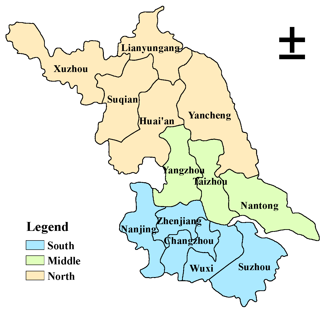
2.2. Variable Selection and Data Collection
- (1)
- Economic scale. Due to the long-term adherence of the development strategies centered on economic construction, the protection of the environment was diluted to a large extent in China. Recently, the government promulgated many environmental regulations, such as the “Five-Year Plan”, Regulations on Promoting the Circular Economy, and Extended Producer Responsibility, and put forward the concept of the “new normal” for the first time in 2014 to slow down the speed of economic development [53]. However, the transformation from an extensive pattern to intensive pattern will take a long time, and economic development still has a significant impact on the environment. Thus, we incorporate the economic scale effect into the model and measure it with per capita GDP.
- (2)
- Industrialization and industrial structure. The combustion of fossil fuels from the secondary industry is an important source of generated sulfur dioxide emissions [22]. Meanwhile, the unreasonable industrial structure leads to the fact that most of Jiangsu’s GDP comes from the secondary industry. In addition, the prosperity of the real estate industry promotes the continuous development of the construction industry, which aggravates the pollution of sulfur dioxide, both directly and indirectly [54]. It is necessary to consider industrialization and the industrial structure as model variables, and we choose gross industrial output value and its proportion to GDP to reflect the impact of industrialization and industrial structure, respectively.
- (3)
- Energy consumption and energy intensity. Energy consumption will increase with the development of industrialization. At present, the energy consumption structure in China is still dominated by petroleum and coal, and large-scale use of these unclean energy sources is the essential factor causing air pollution [55]. On the other hand, energy intensity can be regarded as a reflection of utilization efficiency or technology damage to the environment [56]. The enhancement of process flow or introduction of green technology could reduce energy intensity, which is conducive to decreasing air pollution. In addition, energy intensity has been used as a factor in many studies [21,29,57]. Therefore, energy consumption and energy intensity are also integrated into the model. Referring to Shao et al. [50], we adopt the proportion of energy consumption to gross industrial output value to represent the energy intensity.
2.3. Decomposition Model Based on GDIM
3. Results and Discussion
3.1. The Evolution of Absolute Indicators
3.2. The Evolution of Relative Indicators
3.3. Decomposition Results
3.3.1. Chain-Linked Decomposition
3.3.2. Stage Decomposition
4. Policy Inspirations
- (1)
- Implementing the targeted strategies for the management of industrial sulfur dioxide emissions. By observing the spatial distribution and decomposition results of industrial sulfur dioxide emissions in different regions during 2004–2016, the sulfur emissions present obvious spatial heterogeneity. Thus, it is necessary to implement tailored emission reduction policies in different regions, depending on the relevant factors affecting variations and their location advantages, so as to promote the coupling of development of the environment and economy with high quality.
- (2)
- The GDIM used in this paper indicates that two factors (industrial structure effect and energy intensity effect) have a weak impact on the reduction of industrial sulfur dioxide emissions, which means they can still be further optimized. In fact, traditional high energy consumption and high emissions are signals of economic waste and inefficiency of resources. Relevant industries should adopt a reasonable method of resource transformation. For instance, relying on material resources to attract knowledge and human resources, thereby improving resource potential, or, referring to industrial symbiosis theory or typical eco-industrial park patterns to accelerate the transformation and upgrade traditional industries.
- (3)
- Despite the various measures employed by the Jiangsu provincial government in the field of ecological management, including amending the “Environmental Protection Law” and promulgating the 13th “Five-Year Plan” (2016–2020), the high energy consumption and coal-based energy structure will continue for a long time. Therefore, the government should not only concentrate on end-of-pipe treatment, but also implement the ideology of “environmental protection” into the whole life cycle of products. Meanwhile, the production-oriented enterprises should be regarded as the main factor controlling industrial sulfur dioxide emissions, so as to extend their responsibility for emission reduction and eliminate backward production capacity. In addition, the technologies for long-distance transport and energy storage need to be developed to raise the proportion of renewable energy supply.
5. Conclusions
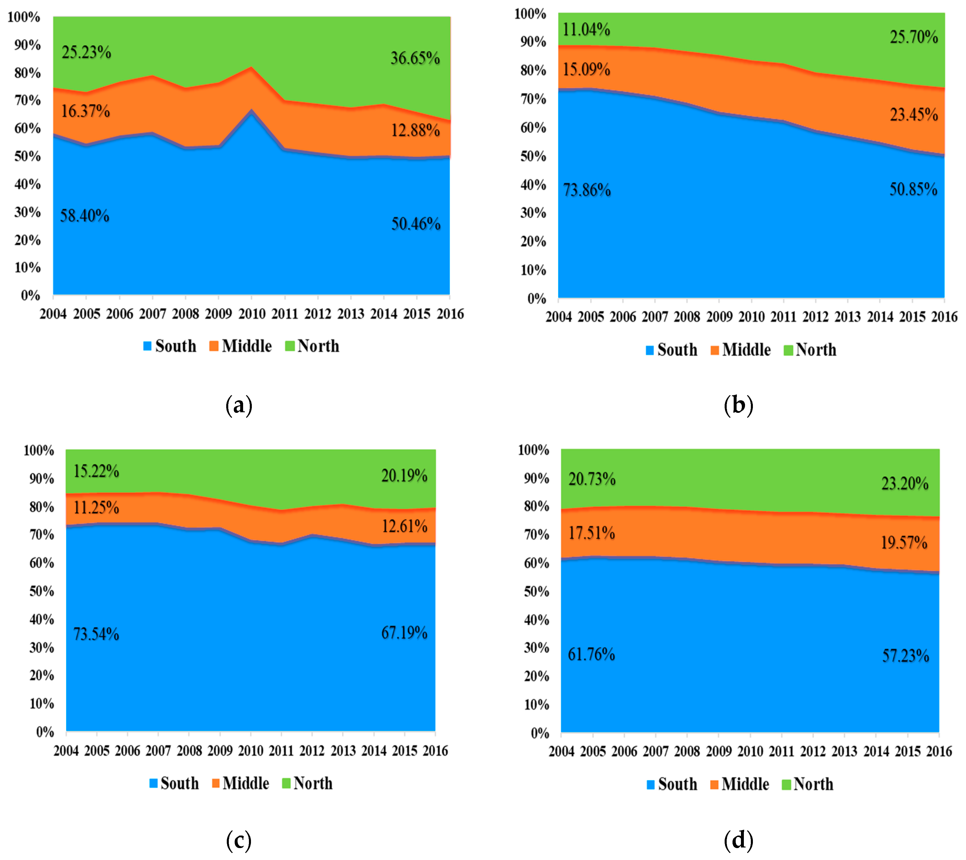
- (1)
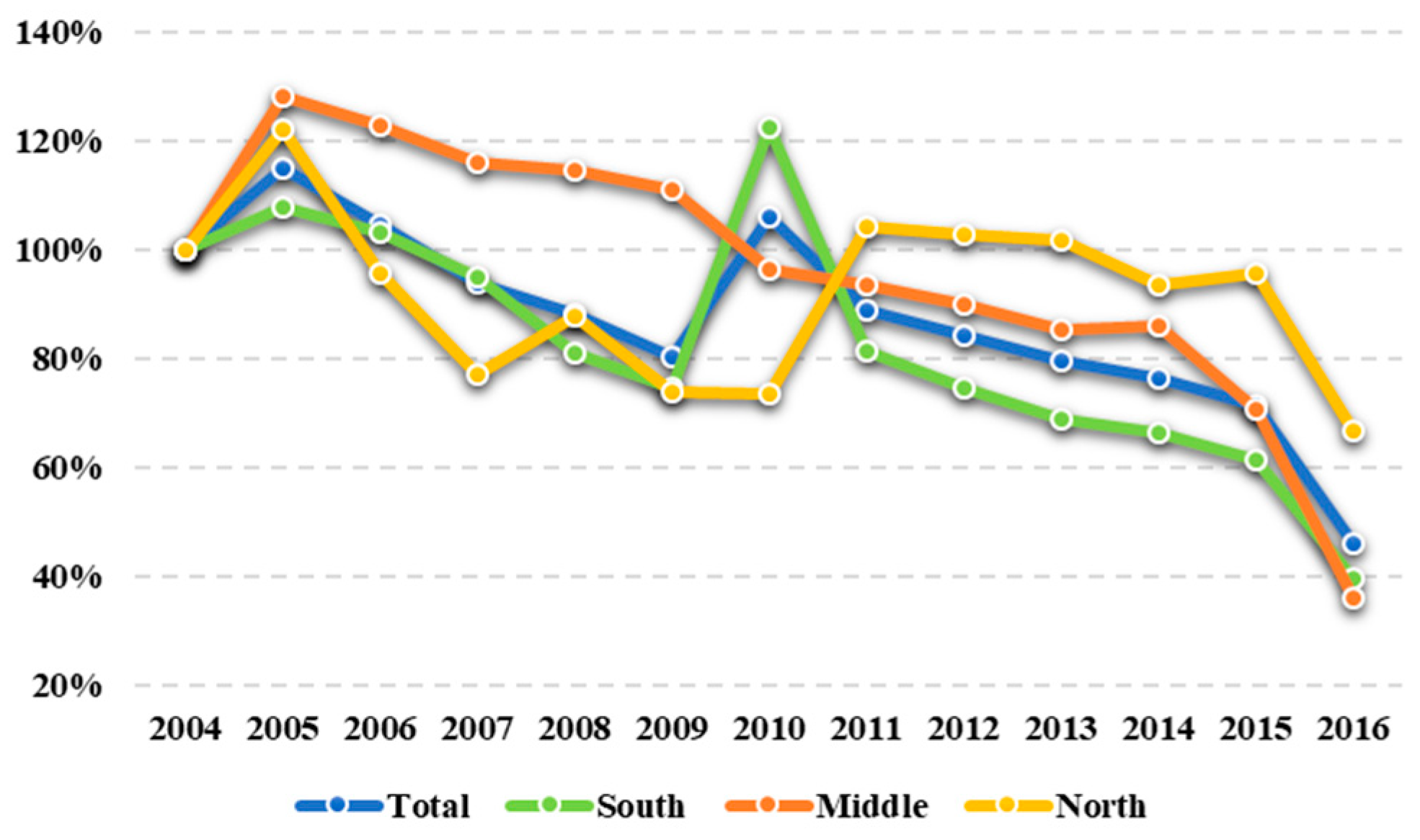
- The share of each region in the total industrial sulfur dioxide emissions evolved with the trend, except in 2010. Although the share of the South region has declined by about 8% (from 58.40% in 2004 to 50.46% in 2016), it still accounts for more than half of the total share. The share of the Middle region also decreased (from 16.37% in 2004 to 12.88% in 2016), while that of the North region increased from 25.23% in 2004 up to 36.65% in 2016.
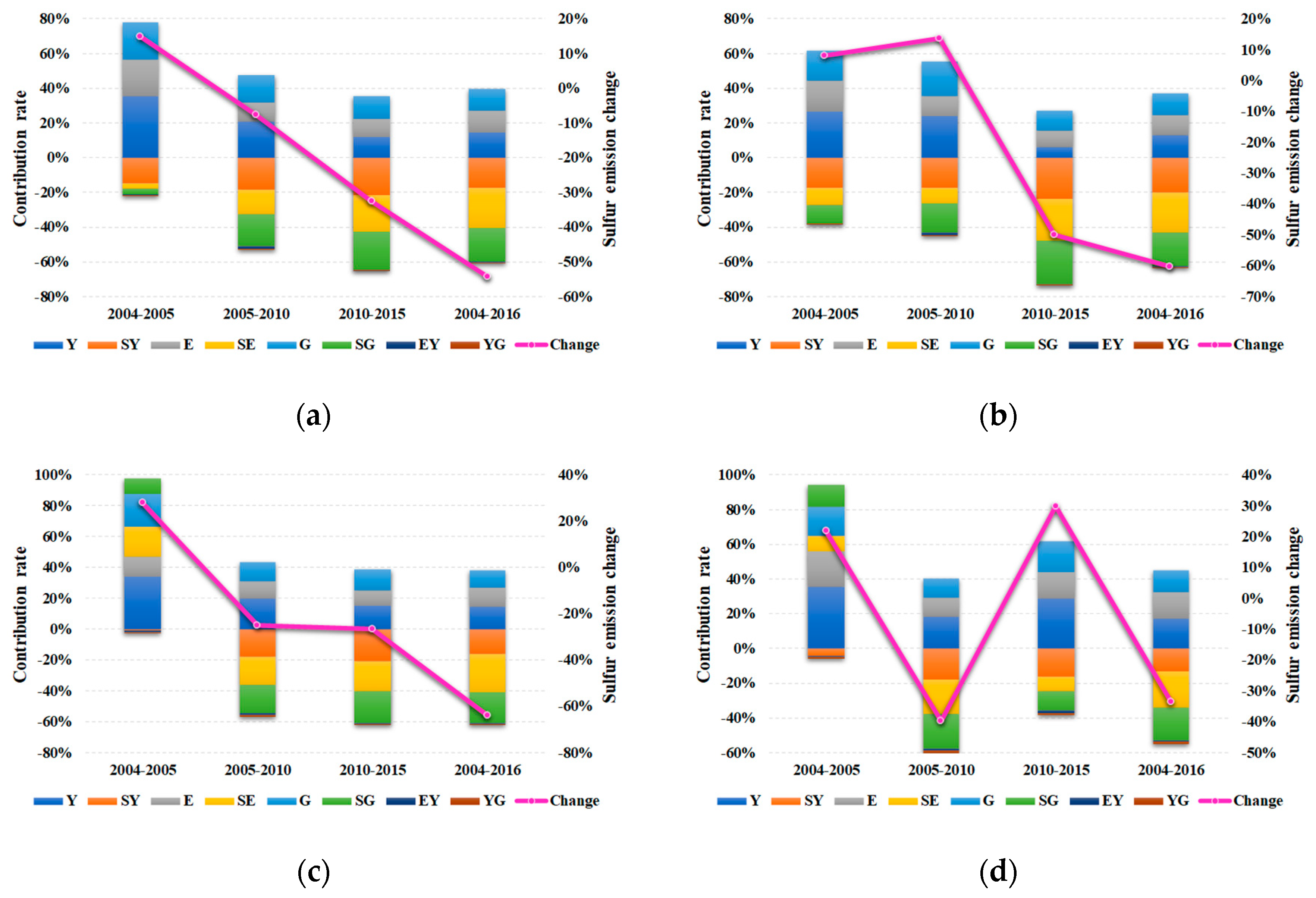
- (2)
- In general, the industrialization effect, economic scale effect, and energy consumption effect of Jiangsu province and its three regions promote industrial sulfur dioxide emissions, whereas the remaining factors, namely the technology effect, sulfur efficiency effect, energy mix effect, energy intensity effect, and industrial structure effect, play mitigating roles in the emissions.
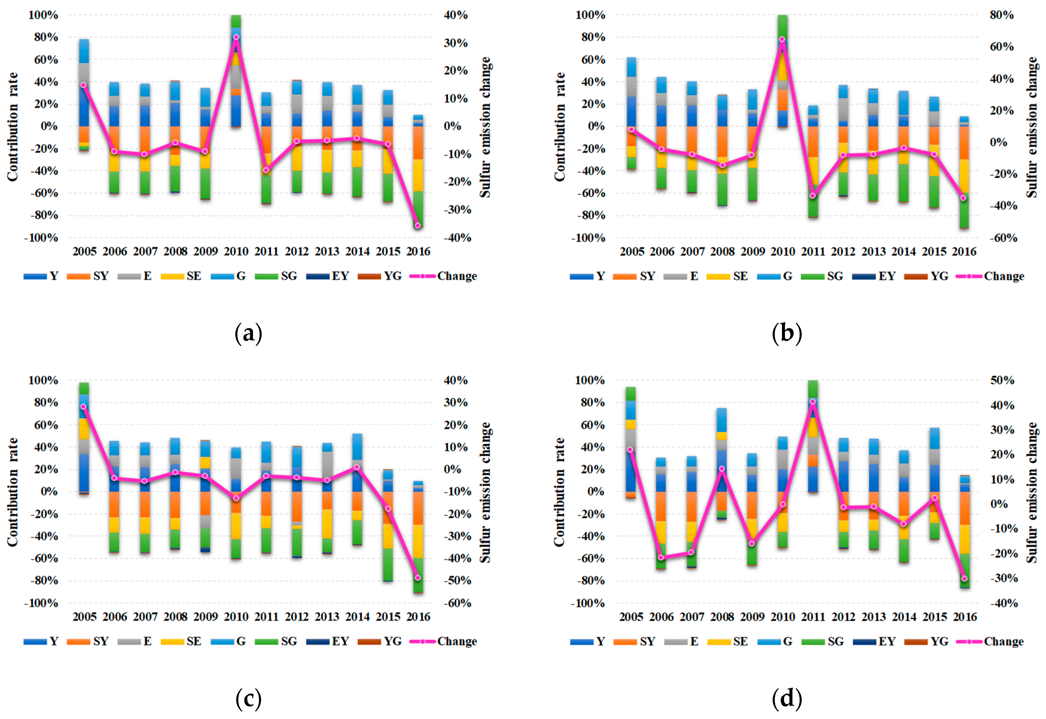
- (3)
- The results of chain-linked decomposition in the South, Middle, and North regions demonstrate that several factors may show anomalous contribution direction. For the South and North regions, this phenomenon mainly occurred in 2010 and 2011, respectively. Specifically, the technology effect, energy mix effect, and sulfur efficiency effect unexpectedly promote industrial sulfur dioxide emissions rather than mitigate them. Regarding the Middle region, it is not easy to comprehend that the energy mix effect and industrial structure effect act as facilitators in 2009, while the energy consumption effect acts as an inhibitor. In addition, by comparing these three regions, the technology effect in the Middle region is not as anomalous as the other two regions. Similarly, the energy consumption effect in the North region promotes industrial sulfur dioxide emissions all the time.
Author Contributions
Funding
Conflicts of Interest
Appendix A

| Y | SY | E | SE | G | SG | EY | YG | Change | |
|---|---|---|---|---|---|---|---|---|---|
| 2004–2005 | 0.0926 | −0.0390 | 0.0562 | −0.0079 | 0.0565 | −0.0085 | −0.0011 | −0.0012 | 0.1476 |
| 2005–2006 | 0.0780 | −0.1017 | 0.0420 | −0.0747 | 0.0527 | −0.0845 | −0.0014 | −0.0006 | −0.0901 |
| 2006–2007 | 0.0836 | −0.1087 | 0.0366 | −0.0736 | 0.0523 | −0.0881 | −0.0024 | −0.0008 | −0.1013 |
| 2007–2008 | 0.0642 | −0.0789 | 0.0069 | −0.0287 | 0.0509 | −0.0708 | −0.0042 | 0.0000 | −0.0606 |
| 2008–2009 | 0.0419 | −0.0700 | 0.0075 | −0.0390 | 0.0478 | −0.0761 | −0.0019 | −0.0001 | −0.0898 |
| 2009–2010 | 0.0897 | 0.0179 | 0.0672 | 0.0389 | 0.0709 | 0.0352 | −0.0004 | −0.0003 | 0.3191 |
| 2010–2011 | 0.0486 | −0.1000 | 0.0266 | −0.0822 | 0.0515 | −0.1032 | −0.0008 | 0.0000 | −0.1595 |
| 2011–2012 | 0.0348 | −0.0542 | 0.0512 | −0.0680 | 0.0385 | −0.0570 | −0.0004 | 0.0000 | −0.0551 |
| 2012–2013 | 0.0355 | −0.0523 | 0.0316 | −0.0491 | 0.0304 | −0.0479 | 0.0000 | 0.0000 | −0.0518 |
| 2013–2014 | 0.0213 | −0.0356 | 0.0104 | −0.0252 | 0.0286 | −0.0424 | −0.0002 | −0.0001 | −0.0432 |
| 2014–2015 | 0.0155 | −0.0372 | 0.0193 | −0.0405 | 0.0239 | −0.0449 | 0.0000 | −0.0001 | −0.0641 |
| 2015–2016 | 0.0137 | −0.1337 | 0.0108 | −0.1312 | 0.0229 | −0.1399 | 0.0000 | −0.0002 | −0.3576 |
| 2005–2010 | 0.3269 | −0.2861 | 0.1695 | −0.2226 | 0.2416 | −0.2788 | −0.0250 | −0.0032 | −0.0777 |
| 2010–2015 | 0.1345 | −0.2428 | 0.1206 | −0.2370 | 0.1478 | −0.2479 | −0.0004 | −0.0004 | −0.3257 |
| 2004–2016 | 0.3710 | −0.4550 | 0.3233 | −0.5944 | 0.3244 | −0.4929 | −0.0168 | −0.0011 | −0.5415 |
| Y | SY | E | SE | G | SG | EY | YG | Change | |
|---|---|---|---|---|---|---|---|---|---|
| 2004–2005 | 0.0902 | −0.0593 | 0.0588 | −0.0338 | 0.0595 | −0.0346 | −0.0009 | −0.0009 | 0.0790 |
| 2005–2006 | 0.0727 | −0.0834 | 0.0427 | −0.0594 | 0.0537 | −0.0697 | −0.0010 | −0.0003 | −0.0446 |
| 2006–2007 | 0.0775 | −0.0974 | 0.0368 | −0.0659 | 0.0526 | −0.0805 | −0.0019 | −0.0005 | −0.0791 |
| 2007–2008 | 0.0496 | −0.0941 | −0.0003 | −0.0514 | 0.0461 | −0.0937 | −0.0037 | 0.0000 | −0.1474 |
| 2008–2009 | 0.0271 | −0.0535 | 0.0077 | −0.0353 | 0.0432 | −0.0678 | −0.0007 | −0.0005 | −0.0799 |
| 2009–2010 | 0.0902 | 0.1245 | 0.0489 | 0.1671 | 0.0752 | 0.1402 | −0.0014 | −0.0001 | 0.6445 |
| 2010–2011 | 0.0371 | −0.1479 | 0.0188 | −0.1353 | 0.0445 | −0.1534 | −0.0007 | −0.0002 | −0.3370 |
| 2011–2012 | 0.0159 | −0.0468 | 0.0675 | −0.0888 | 0.0383 | −0.0656 | −0.0039 | −0.0003 | −0.0837 |
| 2012–2013 | 0.0231 | −0.0488 | 0.0234 | −0.0490 | 0.0277 | −0.0529 | 0.0000 | 0.0000 | −0.0766 |
| 2013–2014 | 0.0092 | −0.0215 | 0.0012 | −0.0136 | 0.0224 | −0.0340 | −0.0001 | −0.0003 | −0.0366 |
| 2014–2015 | 0.0006 | −0.0264 | 0.0216 | −0.0457 | 0.0208 | −0.0451 | −0.0006 | −0.0005 | −0.0753 |
| 2015–2016 | 0.0056 | −0.1253 | 0.0108 | −0.1284 | 0.0207 | −0.1356 | 0.0000 | −0.0004 | −0.3527 |
| 2005–2010 | 0.3170 | −0.2305 | 0.1503 | −0.1146 | 0.2587 | −0.2195 | −0.0259 | −0.0004 | 0.1351 |
| 2010–2015 | 0.0676 | −0.2573 | 0.1029 | −0.2622 | 0.1203 | −0.2665 | −0.0014 | −0.0036 | −0.5002 |
| 2004–2016 | 0.3030 | −0.4604 | 0.2607 | −0.5379 | 0.2911 | −0.4507 | −0.0092 | −0.0005 | −0.6038 |
| Y | SY | E | SE | G | SG | EY | YG | Change | |
|---|---|---|---|---|---|---|---|---|---|
| 2004–2005 | 0.1001 | −0.0022 | 0.0382 | 0.0562 | 0.0625 | 0.0307 | −0.0033 | −0.0010 | 0.2812 |
| 2005–2006 | 0.1027 | −0.1055 | 0.0470 | −0.0642 | 0.0582 | −0.0753 | −0.0029 | −0.0018 | −0.0419 |
| 2006–2007 | 0.1055 | −0.1112 | 0.0485 | −0.0701 | 0.0571 | −0.0789 | −0.0030 | −0.0023 | −0.0544 |
| 2007–2008 | 0.0928 | −0.0881 | 0.0314 | −0.0384 | 0.0549 | −0.0616 | −0.0038 | −0.0011 | −0.0141 |
| 2008–2009 | 0.0725 | −0.0736 | −0.0415 | 0.0360 | 0.0503 | −0.0604 | −0.0153 | 0.0001 | −0.0318 |
| 2009–2010 | 0.0708 | −0.1186 | 0.1155 | −0.1475 | 0.0597 | −0.1077 | −0.0033 | −0.0005 | −0.1317 |
| 2010–2011 | 0.0546 | −0.0624 | 0.0208 | −0.0321 | 0.0542 | −0.0633 | −0.0016 | 0.0000 | −0.0298 |
| 2011–2012 | 0.0437 | −0.0531 | −0.0064 | −0.0060 | 0.0359 | −0.0480 | −0.0034 | 0.0001 | −0.0372 |
| 2012–2013 | 0.0458 | −0.0661 | 0.1050 | −0.1104 | 0.0331 | −0.0526 | −0.0057 | −0.0007 | −0.0516 |
| 2013–2014 | 0.0323 | −0.0295 | 0.0167 | −0.0146 | 0.0400 | −0.0368 | −0.0004 | −0.0001 | 0.0076 |
| 2014–2015 | 0.0283 | −0.0860 | 0.0042 | −0.0657 | 0.0258 | −0.0849 | −0.0009 | 0.0000 | −0.1792 |
| 2015–2016 | 0.0179 | −0.1815 | 0.0168 | −0.1807 | 0.0245 | −0.1848 | 0.0000 | −0.0001 | −0.4879 |
| 2005–2010 | 0.3695 | −0.3328 | 0.2071 | −0.3330 | 0.2286 | −0.3476 | −0.0238 | −0.0170 | −0.2491 |
| 2010–2015 | 0.1816 | −0.2507 | 0.1228 | −0.2296 | 0.1621 | −0.2489 | −0.0045 | 0.0000 | −0.2673 |
| 2004–2016 | 0.3877 | −0.4427 | 0.3385 | −0.6652 | 0.3112 | −0.5388 | −0.0210 | −0.0088 | −0.6390 |
| Y | SY | E | SE | G | SG | EY | YG | Change | |
|---|---|---|---|---|---|---|---|---|---|
| 2004–2005 | 0.0880 | −0.0110 | 0.0506 | 0.0222 | 0.0412 | 0.0319 | −0.0010 | −0.0022 | 0.2196 |
| 2005–2006 | 0.0871 | −0.1457 | 0.0380 | −0.1151 | 0.0461 | −0.1225 | −0.0025 | −0.0018 | −0.2163 |
| 2006–2007 | 0.0947 | −0.1430 | 0.0279 | −0.0989 | 0.0469 | −0.1163 | −0.0047 | −0.0022 | −0.1957 |
| 2007–2008 | 0.1059 | −0.0501 | 0.0268 | 0.0207 | 0.0614 | −0.0155 | −0.0057 | −0.0014 | 0.1421 |
| 2008–2009 | 0.0760 | −0.1228 | 0.0396 | −0.0968 | 0.0586 | −0.1128 | −0.0017 | −0.0002 | −0.1601 |
| 2009–2010 | 0.1145 | −0.1078 | 0.0978 | −0.0988 | 0.0702 | −0.0753 | 0.0000 | −0.0025 | −0.0020 |
| 2010–2011 | 0.0952 | 0.0438 | 0.0649 | 0.0733 | 0.0735 | 0.0645 | −0.0007 | −0.0003 | 0.4141 |
| 2011–2012 | 0.0932 | −0.0866 | 0.0289 | −0.0356 | 0.0404 | −0.0476 | −0.0038 | −0.0027 | −0.0138 |
| 2012–2013 | 0.0595 | −0.0588 | 0.0192 | −0.0238 | 0.0351 | −0.0394 | −0.0018 | −0.0005 | −0.0105 |
| 2013–2014 | 0.0409 | −0.0674 | 0.0381 | −0.0652 | 0.0354 | −0.0629 | 0.0000 | 0.0000 | −0.0812 |
| 2014–2015 | 0.0379 | −0.0293 | 0.0219 | −0.0145 | 0.0300 | −0.0224 | −0.0003 | 0.0000 | 0.0232 |
| 2015–2016 | 0.0262 | −0.1247 | 0.0063 | −0.1100 | 0.0257 | −0.1253 | −0.0007 | 0.0000 | −0.3025 |
| 2005–2010 | 0.3671 | −0.3553 | 0.2153 | −0.3982 | 0.2137 | −0.3956 | −0.0197 | −0.0240 | −0.3966 |
| 2010–2015 | 0.3580 | −0.2033 | 0.1952 | −0.1024 | 0.2221 | −0.1439 | −0.0160 | −0.0125 | 0.2973 |
| 2004–2016 | 0.5651 | −0.4335 | 0.5184 | −0.7065 | 0.4121 | −0.6158 | −0.0263 | −0.0476 | −0.3340 |
References
- Tilt, B. China’s air pollution crisis: Science and policy perspectives. Environ. Sci. Policy 2019, 92, 275–280. [Google Scholar] [CrossRef]
- Ministry of Ecology and Environment. Bulletin on China’s Ecological Environment (2018); China Environmental Press: Beijing, China, 2019.
- Yun, J.; Zhu, C.; Wang, Q.; Hu, Q.; Yang, G. Catalytic conversions of atmospheric sulfur dioxide and formation of acid rain over mineral dusts: Molecular oxygen as the oxygen source. Chemosphere 2019, 217, 18–25. [Google Scholar] [CrossRef] [PubMed]
- Caputo, J.; Beier, C.M.; Sullivan, T.J.; Lawrence, G.B. Modeled effects of soil acidification on long-term ecological and economic outcomes for managed forests in the Adirondack region (USA). Sci. Total Environ. 2016, 565, 401–411. [Google Scholar] [CrossRef] [PubMed]
- Xie, E.; Zhao, Y.; Li, H.; Shi, X.; Lu, F.; Zhang, X.; Peng, Y. Spatio-temporal changes of cropland soil pH in a rapidly industrializing region in the Yangtze River Delta of China, 1980–2015. Agric. Ecosyst. Environ. 2019, 272, 95–104. [Google Scholar] [CrossRef]
- Chen, S.; Li, Y.; Yao, Q. The health costs of the industrial leap forward in China: Evidence from the sulfur dioxide emissions of coal-fired power stations. China Econ. Rev. 2018, 49, 68–83. [Google Scholar] [CrossRef]
- Baumann, H.; Boons, F.; Bragd, A. Mapping the green product development field: Engineering, policy and business perspectives. J. Clean. Prod. 2002, 10, 409–425. [Google Scholar] [CrossRef]
- Bovea, M.D.; Pérez-Belis, V. A taxonomy of ecodesign tools for integrating environmental requirements into the product design process. J. Clean. Prod. 2012, 20, 61–71. [Google Scholar] [CrossRef]
- Dües, C.M.; Tan, K.H.; Lim, M. Green as the new Lean: How to use Lean practices as a catalyst to greening your supply chain. J. Clean. Prod. 2013, 40, 93–100. [Google Scholar] [CrossRef]
- Oliveira, G.A.; Tan, K.H.; Guedes, B.T. Lean and green approach: An evaluation tool for new product development focused on small and medium enterprises. Int. J. Prod. Econ. 2018, 205, 62–73. [Google Scholar] [CrossRef]
- Tseng, M.-L.; Tan, K.-H.; Lim, M.; Lin, R.-J.; Geng, Y. Benchmarking eco-efficiency in green supply chain practices in uncertainty. Prod. Plan. Control. 2014, 25, 1079–1090. [Google Scholar] [CrossRef]
- Lu, Z.; Zhang, Q.; Streets, D.G. Sulfur dioxide and primary carbonaceous aerosol emissions in China and India, 1996–2010. Atmos. Chem. Phys. 2011, 11, 9839–9864. [Google Scholar] [CrossRef]
- The State Council. Energy Saving and Emission Reduction Comprehensive Work in 13th “Five-Year Plan”. Available online: http://www.gov.cn/zhengce/content/2017-01/05/content_5156789.htm (accessed on 16 July 2019).
- The State Council. Eco-Environmental Protection Programme in 13th “Five-Year Plan”. Available online: http://www.gov.cn/zhengce/content/2016-12/05/content_5143290.htm (accessed on 16 July 2019).
- Liu, Q.; Wang, Q. Reexamine SO2 emissions embodied in China’s exports using multiregional input–output analysis. Ecol. Econ. 2015, 113, 39–50. [Google Scholar] [CrossRef]
- Ling, Z.; Huang, T.; Li, J.; Zhou, S.; Lian, L.; Wang, J.; Zhao, Y.; Mao, X.; Gao, H.; Ma, J. Sulfur dioxide pollution and energy justice in Northwestern China embodied in West-East Energy Transmission of China. Appl. Energy 2019, 238, 547–560. [Google Scholar] [CrossRef]
- Qian, Y.; Behrens, P.; Tukker, A.; Rodrigues, J.F.D.; Li, P.; Scherer, L. Environmental responsibility for sulfur dioxide emissions and associated biodiversity loss across Chinese provinces. Environ. Pollut. 2019, 245, 898–908. [Google Scholar] [CrossRef]
- Wang, Z.; Li, C.; Liu, Q.; Niu, B.; Peng, S.; Deng, L.; Kang, P.; Zhang, X. Pollution haven hypothesis of domestic trade in China: A perspective of SO2 emissions. Sci. Total Environ. 2019, 663, 198–205. [Google Scholar] [CrossRef]
- Zhang, Q.; Nakatani, J.; Shan, Y.; Moriguchi, Y. Inter-regional spillover of China’s sulfur dioxide (SO2) pollution across the supply chains. J. Clean. Prod. 2019, 207, 418–431. [Google Scholar] [CrossRef]
- Ramakrishnan, S.; Hishan, S.S.; Nabi, A.A.; Arshad, Z.; Kanjanapathy, M.; Zaman, K.; Khan, F. An interactive environmental model for economic growth: Evidence from a panel of countries. Environ. Sci. Pollut. Res. 2016, 23, 14567–14579. [Google Scholar] [CrossRef]
- Wang, Y.; Han, R.; Kubota, J. Is there an Environmental Kuznets Curve for SO2 emissions? A semi-parametric panel data analysis for China. Renew. Sustain. Energy Rev. 2016, 54, 1182–1188. [Google Scholar] [CrossRef]
- Zhao, X.; Deng, C.; Huang, X.; Kwan, M.-P. Driving forces and the spatial patterns of industrial sulfur dioxide discharge in China. Sci. Total Environ. 2017, 577, 279–288. [Google Scholar] [CrossRef]
- Zhu, L.; Gan, Q.; Liu, Y.; Yan, Z. The impact of foreign direct investment on SO2 emissions in the Beijing-Tianjin-Hebei region: A spatial econometric analysis. J. Clean. Prod. 2017, 166, 189–196. [Google Scholar] [CrossRef]
- Huang, J.-T. Sulfur dioxide (SO2) emissions and government spending on environmental protection in China—Evidence from spatial econometric analysis. J. Clean. Prod. 2018, 175, 431–441. [Google Scholar] [CrossRef]
- Ahmed Bhuiyan, M.; Rashid Khan, H.U.; Zaman, K.; Hishan, S.S. Measuring the impact of global tropospheric ozone, carbon dioxide and sulfur dioxide concentrations on biodiversity loss. Environ. Res. 2018, 160, 398–411. [Google Scholar] [CrossRef] [PubMed]
- Hu, B.; Li, Z.; Zhang, L. Long-run dynamics of sulphur dioxide emissions, economic growth, and energy efficiency in China. J. Clean. Prod. 2019, 227, 942–949. [Google Scholar] [CrossRef]
- Jiao, J.; Han, X.; Li, F.; Bai, Y.; Yu, Y. Contribution of demand shifts to industrial SO2 emissions in a transition economy: Evidence from China. J. Clean. Prod. 2017, 164, 1455–1466. [Google Scholar] [CrossRef]
- Liu, Q.; Wang, Q. How China achieved its 11th Five-Year Plan emissions reduction target: A structural decomposition analysis of industrial SO2 and chemical oxygen demand. Sci. Total Environ. 2017, 574, 1104–1116. [Google Scholar] [CrossRef]
- Hang, Y.; Wang, Q.; Wang, Y.; Su, B.; Zhou, D. Industrial SO2 emissions treatment in China: A temporal-spatial whole process decomposition analysis. J. Environ. Manag. 2019, 243, 419–434. [Google Scholar] [CrossRef]
- Li, Z.; Shao, S.; Shi, X.; Sun, Y.; Zhang, X. Structural transformation of manufacturing, natural resource dependence, and carbon emissions reduction: Evidence of a threshold effect from China. J. Clean. Prod. 2019, 206, 920–927. [Google Scholar] [CrossRef]
- National Bureau of Statistics. China Statistical Yearbook; China Statistics Press: Jiangsu, China, 2017.
- Jiangsu Provincial Statistics Bureau. Jiangsu Statistical Yearbook (2017); China Statistics Press: Jiangsu, China, 2017.
- People’s Daily. Exploring the Road of Development is the Consistent Requirement of the Central Committee for Jiangsu Province. Available online: http://js.people.com.cn/n/2014/1222/c360300-23295972.html (accessed on 9 October 2019).
- Ministry of Science and Technology. Southern Jiangsu Province was Approved as a Demonstration Zone of National Independent Innovation. Available online: http://www.most.gov.cn/kjbgz/201411/t20141105 _116519.htm (accessed on 9 October 2019).
- Wang, H.; Zhou, P. Assessing Global CO2 Emission Inequality from Consumption Perspective: An Index Decomposition Analysis. Ecol. Econ. 2018, 154, 257–271. [Google Scholar] [CrossRef]
- Wang, H.; Ang, B.W. Assessing the role of international trade in global CO2 emissions: An index decomposition analysis approach. Appl. Energy 2018, 218, 146–158. [Google Scholar] [CrossRef]
- Zhang, C.; Su, B.; Zhou, K.; Yang, S. Analysis of electricity consumption in China (1990–2016) using index decomposition and decoupling approach. J. Clean. Prod. 2019, 209, 224–235. [Google Scholar] [CrossRef]
- Zhou, X.; Zhou, D.; Wang, Q. How does information and communication technology affect China’s energy intensity? A three-tier structural decomposition analysis. Energy 2018, 151, 748–759. [Google Scholar] [CrossRef]
- Magacho, G.R.; McCombie, J.S.L.; Guilhoto, J.J.M. Impacts of trade liberalization on countries’ sectoral structure of production and trade: A structural decomposition analysis. Struct. Chang. Econ. Dyn. 2018, 46, 70–77. [Google Scholar] [CrossRef]
- He, H.; Reynolds, C.J.; Zhou, Z.; Wang, Y.; Boland, J. Changes of waste generation in Australia: Insights from structural decomposition analysis. Waste Manag. 2019, 83, 142–150. [Google Scholar] [CrossRef] [PubMed]
- Su, B.; Ang, B.W. Structural decomposition analysis applied to energy and emissions: Some methodological developments. Energy Econ. 2012, 34, 177–188. [Google Scholar] [CrossRef]
- Wang, H.; Ang, B.W.; Su, B. Assessing drivers of economy-wide energy use and emissions: IDA versus SDA. Energy Policy 2017, 107, 585–599. [Google Scholar] [CrossRef]
- Ang, B.W. Decomposition analysis for policymaking in energy: Which is the preferred method? Energy Policy 2004, 32, 1131–1139. [Google Scholar] [CrossRef]
- Lu, Y.; Cui, P.; Li, D. Which activities contribute most to building energy consumption in China? A hybrid LMDI decomposition analysis from year 2007 to 2015. Energy Build. 2018, 165, 259–269. [Google Scholar] [CrossRef]
- Wang, M.; Feng, C. Decomposing the change in energy consumption in China’s nonferrous metal industry: An empirical analysis based on the LMDI method. Renew. Sustain. Energy Rev. 2018, 82, 2652–2663. [Google Scholar] [CrossRef]
- Zhang, M.; Bai, C.; Zhou, M. Decomposition analysis for assessing the progress in decoupling relationship between coal consumption and economic growth in China. Resour. Conserv. Recycl. 2018, 129, 454–462. [Google Scholar] [CrossRef]
- Chen, W.; Yang, M.; Zhang, S.; Andrews-Speed, P.; Li, W. What accounts for the China–US difference in solar PV electricity output? An LMDI analysis. J. Clean. Prod. 2019, 231, 161–170. [Google Scholar] [CrossRef]
- Liang, W.; Gan, T.; Zhang, W. Dynamic evolution of characteristics and decomposition of factors influencing industrial carbon dioxide emissions in China: 1991–2015. Struct. Chang. Econ. Dyn. 2019, 49, 93–106. [Google Scholar] [CrossRef]
- Vaninsky, A. Factorial decomposition of CO2 emissions: A generalized Divisia index approach. Energy Econ. 2014, 45, 389–400. [Google Scholar] [CrossRef]
- Shao, S.; Liu, J.; Geng, Y.; Miao, Z.; Yang, Y. Uncovering driving factors of carbon emissions from China’s mining sector. Appl. Energy 2016, 166, 220–238. [Google Scholar] [CrossRef]
- Yan, Q.; Wang, Y.; Li, Z.; Baležentis, T.; Streimikiene, D. Coordinated development of thermal power generation in Beijing–Tianjin–Hebei region: Evidence from decomposition and scenario analysis for carbon dioxide emission. J. Clean. Prod. 2019, 232, 1402–1417. [Google Scholar] [CrossRef]
- Yan, Q.; Wang, Y.; Baležentis, T.; Streimikiene, D. Analysis of China’s regional thermal electricity generation and CO2 emissions: Decomposition based on the generalized Divisia index. Sci. Total Environ. 2019, 682, 737–755. [Google Scholar] [CrossRef] [PubMed]
- Tung, R.L. Opportunities and Challenges Ahead of China’s “New Normal”. Long Range Plann. 2016, 49, 632–640. [Google Scholar] [CrossRef]
- Cheng, Z.; Li, L.; Liu, J. Identifying the spatial effects and driving factors of urban PM2.5 pollution in China. Ecol. Indic. 2017, 82, 61–75. [Google Scholar] [CrossRef]
- Lyu, W.; Li, Y.; Guan, D.; Zhao, H.; Zhang, Q.; Liu, Z. Driving forces of Chinese primary air pollution emissions: An index decomposition analysis. J. Clean. Prod. 2016, 133, 136–144. [Google Scholar] [CrossRef]
- Martínez-Zarzoso, I.; Bengochea-Morancho, A.; Morales-Lage, R. The impact of population on CO2 emissions: Evidence from European countries. Environ. Resour. Econ. 2007, 38, 497–512. [Google Scholar] [CrossRef]
- Rafaj, P.; Amann, M.; Siri, J.; Wuester, H. Changes in European greenhouse gas and air pollutant emissions 1960–2010: Decomposition of determining factors. Clim. Chang. 2014, 124, 477–504. [Google Scholar] [CrossRef]
- National Bureau of Statistics. China City Statistical Yearbook (2005–2017); China Statistics Press: Beijing, China, 2017.


| Variables | Definition | Effect |
|---|---|---|
| Industrial sulfur dioxide emissions | Not Applicable | |
| Per capita GDP | Economic scale effect | |
| Gross industrial output value | Industrialization effect | |
| Energy consumption | Energy consumption effect | |
| Sulfur intensity of per capita GDP | Sulfur efficiency effect | |
| Sulfur intensity of gross industrial output value | Technology effect | |
| Sulfur intensity of energy consumption | Energy mix effect | |
| Energy intensity | Energy intensity effect | |
| Industrial structure | Industrial structure effect |
© 2019 by the authors. Licensee MDPI, Basel, Switzerland. This article is an open access article distributed under the terms and conditions of the Creative Commons Attribution (CC BY) license (http://creativecommons.org/licenses/by/4.0/).
Share and Cite
Yang, J.; Shan, H. Identifying Driving Factors of Jiangsu’s Regional Sulfur Dioxide Emissions: A Generalized Divisia Index Method. Int. J. Environ. Res. Public Health 2019, 16, 4004. https://doi.org/10.3390/ijerph16204004
Yang J, Shan H. Identifying Driving Factors of Jiangsu’s Regional Sulfur Dioxide Emissions: A Generalized Divisia Index Method. International Journal of Environmental Research and Public Health. 2019; 16(20):4004. https://doi.org/10.3390/ijerph16204004
Chicago/Turabian StyleYang, Junliang, and Haiyan Shan. 2019. "Identifying Driving Factors of Jiangsu’s Regional Sulfur Dioxide Emissions: A Generalized Divisia Index Method" International Journal of Environmental Research and Public Health 16, no. 20: 4004. https://doi.org/10.3390/ijerph16204004
APA StyleYang, J., & Shan, H. (2019). Identifying Driving Factors of Jiangsu’s Regional Sulfur Dioxide Emissions: A Generalized Divisia Index Method. International Journal of Environmental Research and Public Health, 16(20), 4004. https://doi.org/10.3390/ijerph16204004