Influencing Factors of PM2.5 Pollution: Disaster Points of Meteorological Factors
Abstract
1. Introduction
1.1. Meteorological Factors
1.2. Human Activities
2. Indicator Selection and Data Sources
2.1. Indicator Selection
2.1.1. Meteorological Factors
2.1.2. Human Activities
2.2. Data Sources
3. Model Construction
4. Results and Analyses
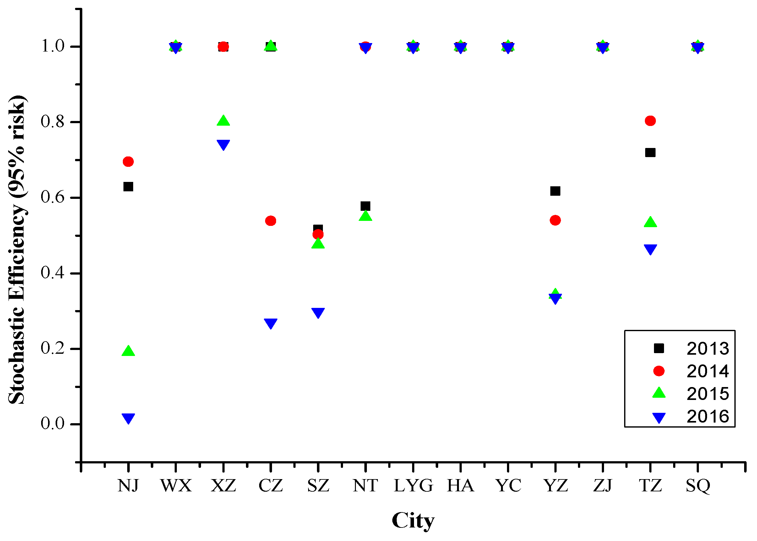
4.1. Stochastic DEA Results for 2013–2016
4.1.1. Year 2013
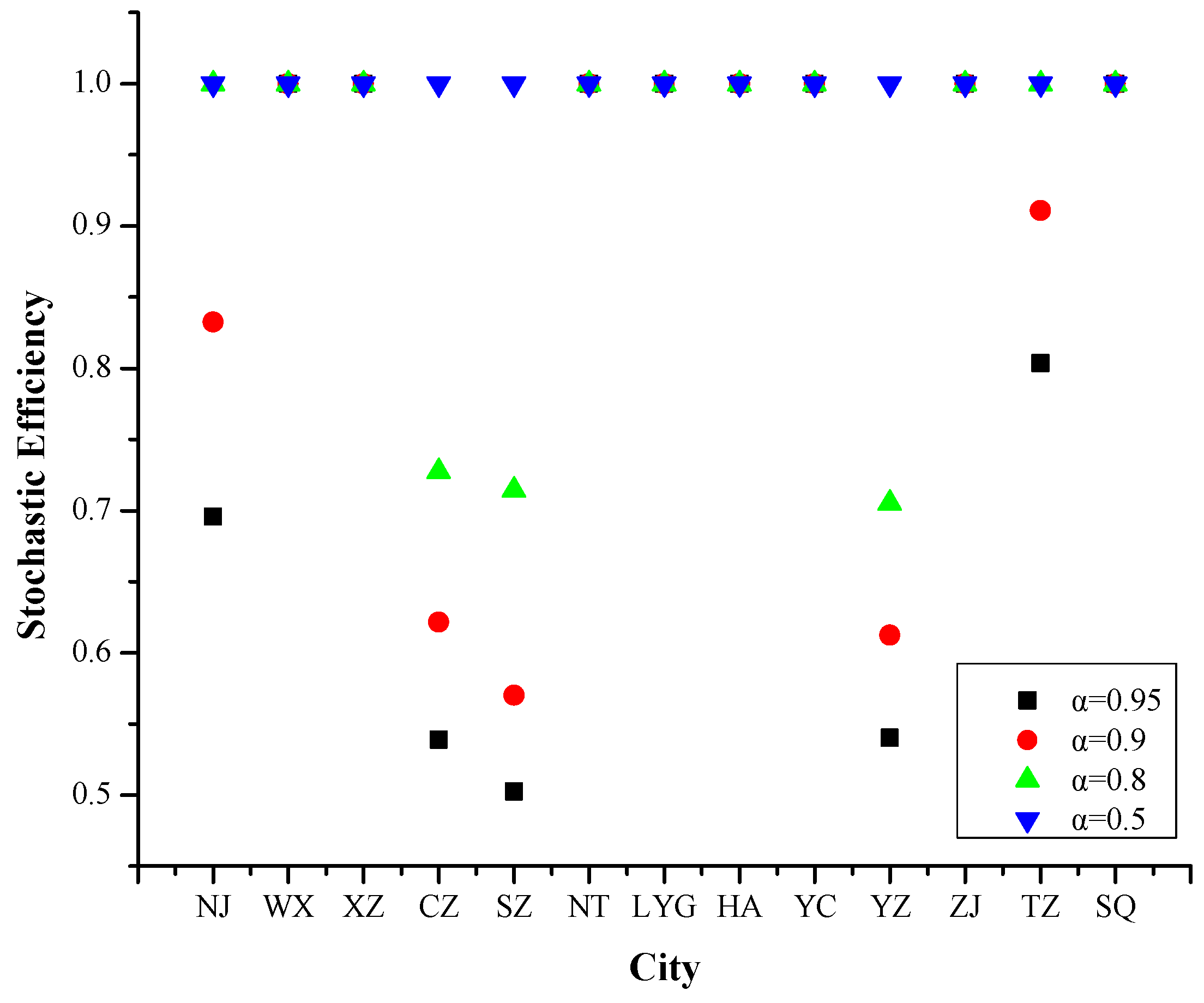
4.1.2. Year 2014
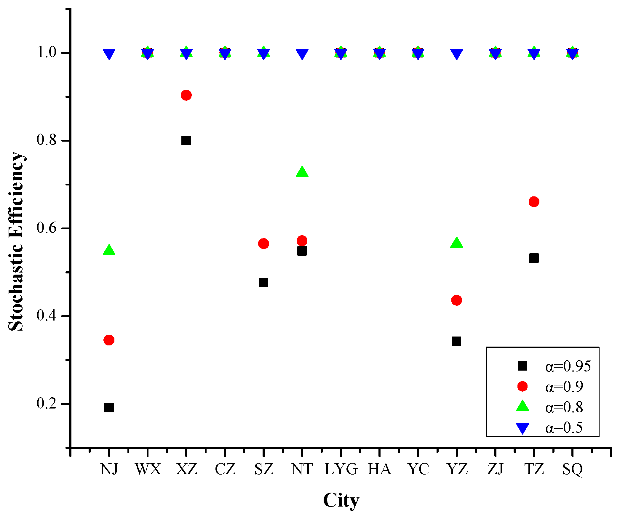
4.1.3. Year 2015
4.1.4. Year 2016
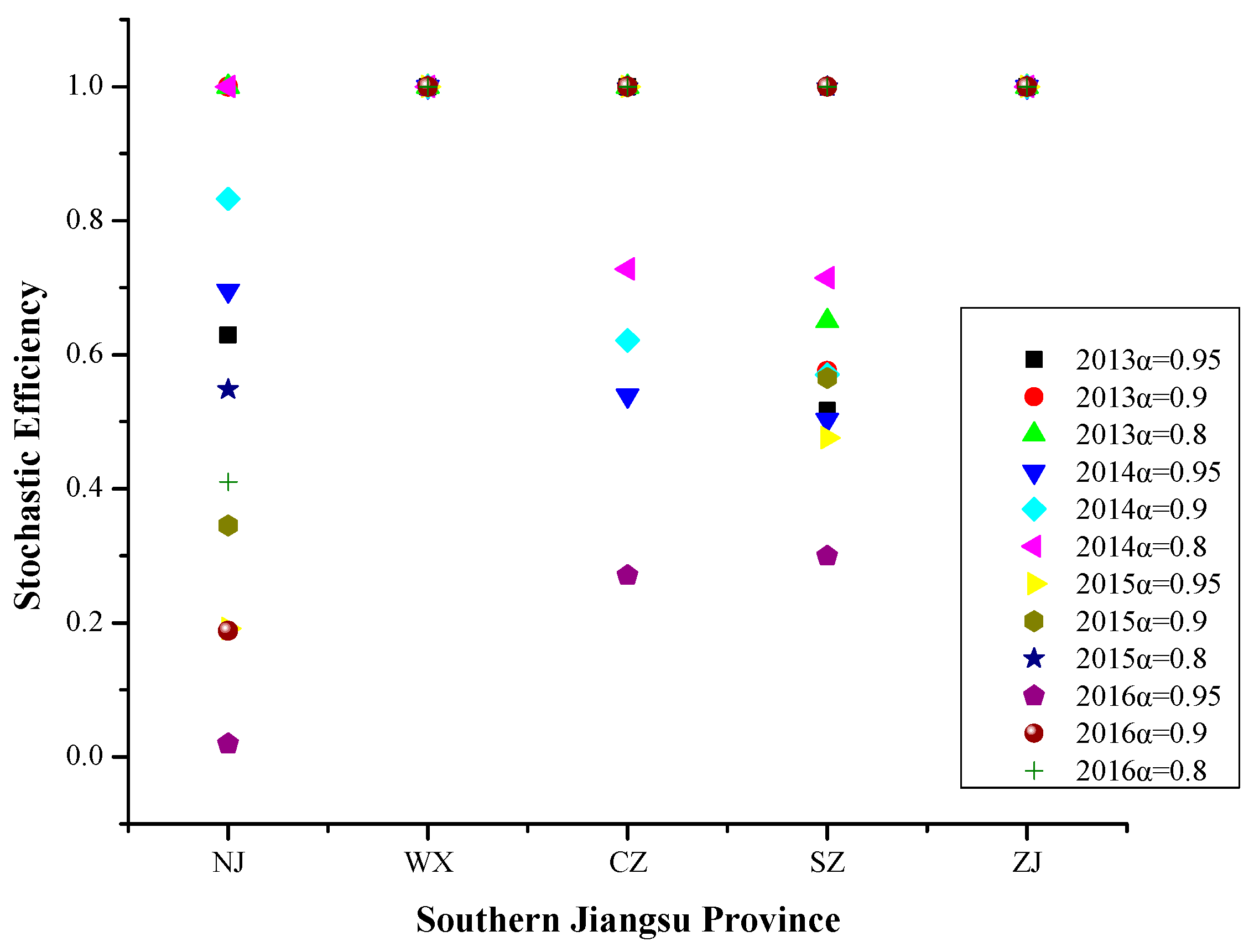
4.2. Regional Stochastic DEA Results
4.2.1. Southern Jiangsu Province
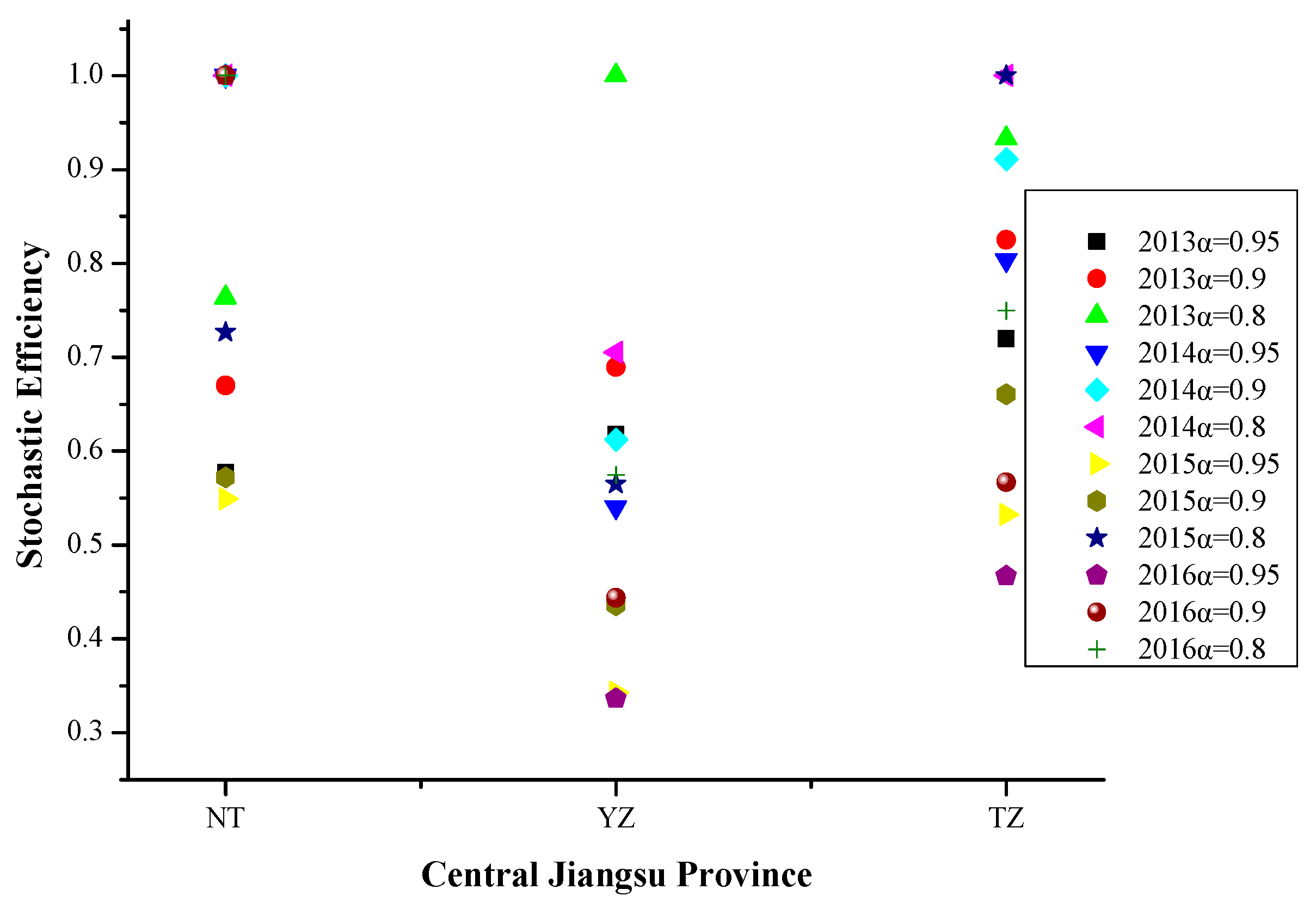
4.2.2. Central Jiangsu Province
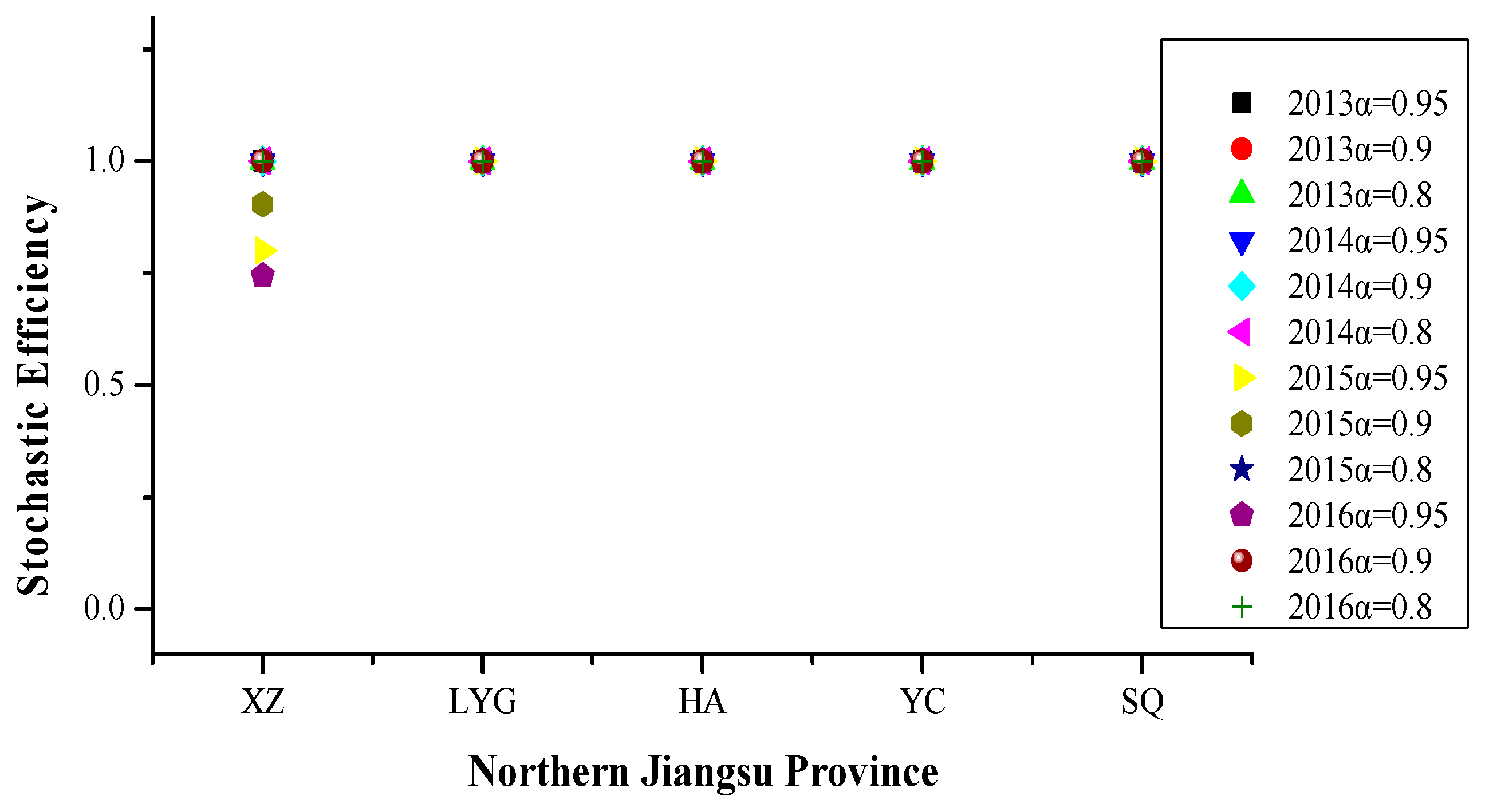
4.2.3. Northern Jiangsu Province
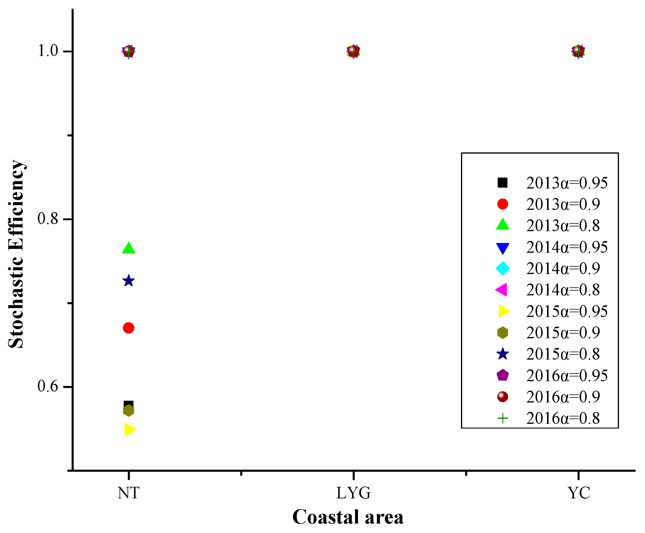
4.2.4. Coastal Area
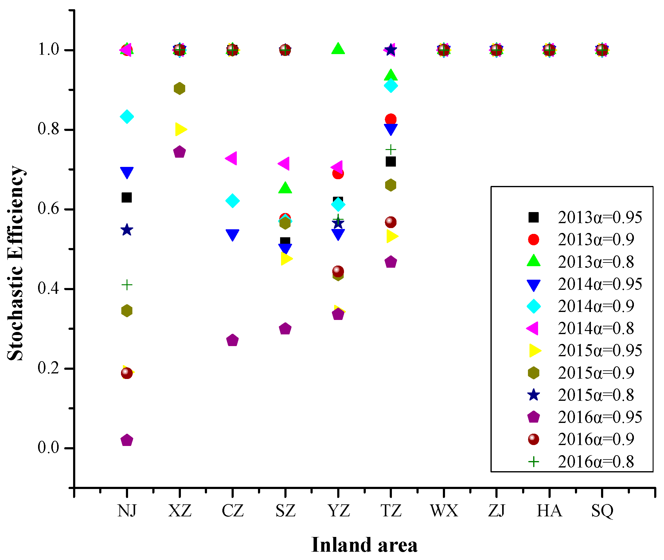
4.2.5. Inland Area
5. Results Comparison
6. Conclusions and Policy Recommendations
6.1. Conclusions
- (1)
- Consider the distribution characteristics of data.
- (2)
- Comprehensively investigate the meteorological factors and human activities.
- (3)
- Differentiate multiple effective decision units.
6.2. Policy Recommendations
Author Contributions
Funding
Acknowledgments
Conflicts of Interest
Appendix A
| Disaster Point Days | 2013 | 2014 | 2015 | 2016 |
|---|---|---|---|---|
| wind speed (<1.5 m/s) | 0.5967 | 0.5237 | 0.5955 | 0.6250 |
| no precipitation day (= 0 mm) | 0.8450 | 0.7868 | 0.7905 | 0.7684 |
| positive temperature change (℃) | 0.8108 | 0.8282 | 0.6977 | 0.6364 |
| negative pressure change (hpa) | 0.8545 | 0.8167 | 0.7033 | 0.6374 |
| relative humidity (60–90%, excluding precipitation days) | 0.6327 | 0.6760 | 0.6122 | 0.5788 |
| DMUs | a = 0.95 | Delete MF | Delete ID | Delete SP | Delete T | Delete EU | Delete EP |
|---|---|---|---|---|---|---|---|
| Nanjing | 0.6957 | 0.6098 | |||||
| Wuxi | 1.0000 | 0.5222 | |||||
| Xuzhou | 1.0000 | 0.6689 | |||||
| Changzhou | 0.5389 | 0.5234 | 0.5361 | ||||
| Suzhou | 0.5025 | 0.5047 | 0.4561 | 0.4770 | |||
| Nantong | 1.0000 | 0.3982 | 0.4915 | ||||
| Lianyungang | 1.0000 | ||||||
| Huai’an | 1.0000 | 0.5820 | 0.7774 | ||||
| Yancheng | 1.0000 | 0.3721 | |||||
| Yangzhou | 0.5401 | 0.5064 | |||||
| Zhenjiang | 1.0000 | 0.5987 | |||||
| Taizhou | 0.8035 | 0.7725 | 0.7753 | 0.7675 | |||
| Suqian | 1.0000 |
| DMUs | a = 0.95 | Delete MF | Delete ID | Delete SP | Delete T | Delete EU | Delete EP |
|---|---|---|---|---|---|---|---|
| Nanjing | 0.1912 | 0.1761 | |||||
| Wuxi | 1.0000 | 0.4562 | |||||
| Xuzhou | 0.8004 | ||||||
| Changzhou | 1.0000 | 0.3855 | |||||
| Suzhou | 0.4761 | 0.4666 | 0.4909 | 0.4849 | |||
| Nantong | 0.5489 | 0.5007 | |||||
| Lianyungang | 1.0000 | 0.4622 | |||||
| Huai’an | 1.0000 | 0.4864 | |||||
| Yancheng | 1.0000 | 0.3725 | |||||
| Yangzhou | 0.3427 | 0.3393 | 0.3151 | ||||
| Zhenjiang | 1.0000 | 0.3984 | |||||
| Taizhou | 0.5322 | 0.5251 | |||||
| Suqian | 1.0000 |
| DMUs | a = 0.95 | Delete MF | Delete ID | Delete SP | Delete T | Delete EU | Delete EP |
|---|---|---|---|---|---|---|---|
| Nanjing | 0.0195 | 0.0187 | |||||
| Wuxi | 1.0000 | 0.3156 | |||||
| Xuzhou | 0.7436 | 0.7186 | |||||
| Changzhou | 0.2706 | 0.2615 | 0.2499 | ||||
| Suzhou | 0.2991 | 0.2833 | 0.2641 | 0.2886 | |||
| Nantong | 1.0000 | 0.2984 | 0.3226 | 0.3226 | |||
| Lianyungang | 1.0000 | ||||||
| Huai’an | 1.0000 | 0.4609 | |||||
| Yancheng | 1.0000 | 0.3222 | |||||
| Yangzhou | 0.3362 | 0.3361 | 0.3424 | 0.3362 | 0.3217 | ||
| Zhenjiang | 1.0000 | 0.1833 | |||||
| Taizhou | 0.4671 | 0.4581 | |||||
| Suqian | 1.0000 |
| DMUs | a = 0.95 | Delete WS | Delete NPD | Delete PTC | Delete NPC | Delete RH | Delete GOVIE | Delete UR |
| Nanjing | 0.6957 | 0.6494 | 0.6098 | |||||
| Wuxi | 1 | |||||||
| Xuzhou | 1 | 0.679 | ||||||
| Changzhou | 0.5389 | |||||||
| Suzhou | 0.5025 | 0.5047 | ||||||
| Nantong | 1 | 0.3982 | ||||||
| Lianyungang | 1 | |||||||
| Huai’an | 1 | |||||||
| Yancheng | 1 | |||||||
| Yangzhou | 0.5401 | |||||||
| Zhenjiang | 1 | |||||||
| Taizhou | 0.8035 | 0.7725 | ||||||
| Suqian | 1 | |||||||
| DMUs | a = 0.95 | Delete PD | Delete BCA | Delete CCO | Delete NPTVO | Delete EC | Delete TCC | Delete GCRBD |
| Nanjing | 0.6957 | |||||||
| Wuxi | 1 | 0.5222 | ||||||
| Xuzhou | 1 | |||||||
| Changzhou | 0.5389 | 0.5234 | 0.5361 | |||||
| Suzhou | 0.5025 | 0.4561 | 0.477 | |||||
| Nantong | 1 | 0.4915 | ||||||
| Lianyungang | 1 | |||||||
| Huai’an | 1 | 0.6079 | 0.7774 | |||||
| Yancheng | 1 | 0.4315 | ||||||
| Yangzhou | 0.5401 | 0.5064 | ||||||
| Zhenjiang | 1 | 0.5987 | ||||||
| Taizhou | 0.8035 | 0.7837 | 0.7675 | |||||
| Suqian | 1 |
| DMUs | a = 0.95 | Delete WS | Delete NPD | Delete PTC | Delete NPC | Delete RH | Delete GOVIE | Delete UR | Delete PD | Delete BCA | Delete CCO | Delete NPTVO | Delete EC | Delete TCC | Delete GCRBD |
|---|---|---|---|---|---|---|---|---|---|---|---|---|---|---|---|
| Nanjing | 0.1912 | 0.1761 | |||||||||||||
| Wuxi | 1.0000 | 0.4562 | |||||||||||||
| Xuzhou | 0.8004 | ||||||||||||||
| Changzhou | 1.0000 | 0.3920 | |||||||||||||
| Suzhou | 0.4761 | 0.4618 | 0.4842 | 0.4761 | 0.4757 | 0.4909 | 0.4849 | ||||||||
| Nantong | 0.5489 | 0.5221 | 0.5364 | ||||||||||||
| Lianyungang | 1.0000 | 0.4622 | |||||||||||||
| Huai’an | 1.0000 | 0.4883 | |||||||||||||
| Yancheng | 1.0000 | 0.4026 | |||||||||||||
| Yangzhou | 0.3427 | 0.3393 | 0.3151 | ||||||||||||
| Zhenjiang | 1.0000 | 0.3984 | |||||||||||||
| Taizhou | 0.5322 | 0.5251 | |||||||||||||
| Suqian | 1.0000 |
| DMUs | a = 0.95 | Delete WS | Delete NPD | Delete PTC | Delete NPC | Delete RH | Delete GOVIE | Delete UR | Delete PD | Delete BCA | Delete CCO | Delete NPTVO | Delete EC | Delete TCC | Delete GCRBD |
|---|---|---|---|---|---|---|---|---|---|---|---|---|---|---|---|
| Nanjing | 0.0195 | 0.0187 | |||||||||||||
| Wuxi | 1.0000 | 0.3156 | |||||||||||||
| Xuzhou | 0.7436 | 0.7186 | |||||||||||||
| Changzhou | 0.2706 | 0.2681 | 0.2564 | ||||||||||||
| Suzhou | 0.2991 | 0.2983 | 1.0000 | 0.2641 | 0.2886 | ||||||||||
| Nantong | 1.0000 | 0.3030 | 0.3060 | 0.3820 | 0.3226 | 0.3226 | |||||||||
| Lianyungang | 1.0000 | ||||||||||||||
| Huai’an | 1.0000 | 0.4609 | 0.5513 | ||||||||||||
| Yancheng | 1.0000 | 0.3488 | |||||||||||||
| Yangzhou | 0.3362 | 0.3361 | 0.3362 | 0.3424 | 0.3362 | 0.3424 | 0.3362 | 0.3217 | |||||||
| Zhenjiang | 1.0000 | ||||||||||||||
| Taizhou | 0.4671 | 0.4581 | |||||||||||||
| Suqian | 1.0000 |
| Years | DMUs | a = 0.95 | Delete MF | Delete ID | Delete SP | Delete T | Delete EU | Delete EP |
|---|---|---|---|---|---|---|---|---|
| 2013 | Nanjing | 0.6294 | 0.5882 | |||||
| Wuxi | 1 | 0.6848 | 0.6259 | |||||
| Xuzhou | 1 | 0.6755 | 0.6428 | |||||
| Suzhou | 0.5162 | 0.5055 | 0.5146 | 0.4946 | ||||
| Zhenjiang | 1 | 0.6199 | ||||||
| 2014 | Nanjing | 0.6957 | 0.6098 | |||||
| Wuxi | 1.0000 | 0.5222 | ||||||
| Xuzhou | 0.5389 | 0.5234 | 0.5361 | |||||
| Suzhou | 0.5025 | 0.5047 | 0.4561 | 0.4770 | ||||
| Zhenjiang | 1.0000 | 0.5987 | ||||||
| 2015 | Nanjing | 0.1912 | 0.1761 | |||||
| Wuxi | 1.0000 | 0.4562 | ||||||
| Xuzhou | 1.0000 | 0.3855 | ||||||
| Suzhou | 0.4761 | 0.4666 | 0.4909 | 0.4849 | ||||
| Zhenjiang | 1.0000 | 0.3984 | ||||||
| 2016 | Nanjing | 0.0195 | 0.0187 | |||||
| Wuxi | 1.0000 | 0.3156 | ||||||
| Xuzhou | 0.2706 | 0.2615 | 0.2499 | |||||
| Suzhou | 0.2991 | 0.2833 | 0.2641 | 0.2886 | ||||
| Zhenjiang | 1.0000 | 0.1833 |
| Years | DMUs | a = 0.95 | Delete MF | Delete ID | Delete SP | Delete T | Delete EU | Delete EP |
|---|---|---|---|---|---|---|---|---|
| 2013 | Nantong | 0.5776 | 0.6129 | 0.5708 | 1 | |||
| Yangzhou | 0.6181 | 0.6062 | 0.6122 | |||||
| Taizhou | 0.7197 | 0.6883 | 0.7265 | 0.641 | 0.722 | |||
| 2014 | Nantong | 1.0000 | 0.3982 | 0.4915 | ||||
| Yangzhou | 0.5401 | 0.5064 | ||||||
| Taizhou | 0.8035 | 0.7725 | 0.7753 | 0.7675 | ||||
| 2015 | Nantong | 0.5489 | 0.5007 | |||||
| Yangzhou | 0.3427 | 0.3393 | 0.3151 | |||||
| Taizhou | 0.5322 | 0.5251 | ||||||
| 2016 | Nantong | 1.0000 | 0.2984 | 0.3226 | 0.3226 | |||
| Yangzhou | 0.3362 | 0.3361 | 0.3424 | 0.3362 | 0.3217 | |||
| Taizhou | 0.4671 | 0.4581 |
| Years | DMUs | a = 0.95 | Delete MF | Delete ID | Delete SP | Delete T | Delete EU | Delete EP |
|---|---|---|---|---|---|---|---|---|
| 2013 | Xuzhou | 1.0000 | 0.7798 | |||||
| Lianyungang | 1.0000 | |||||||
| Huai’an | 1.0000 | 0.6927 | 0.8089 | |||||
| Yancheng | 1.0000 | 0.6284 | ||||||
| Suqian | 1.0000 | |||||||
| 2014 | Xuzhou | 1.0000 | 0.6689 | |||||
| Lianyungang | 1.0000 | |||||||
| Huai’an | 1.0000 | 0.5820 | 0.7774 | |||||
| Yancheng | 1.0000 | 0.3721 | ||||||
| Suqian | 1.0000 | |||||||
| 2015 | Xuzhou | 0.8004 | ||||||
| Lianyungang | 1.0000 | 0.4622 | ||||||
| Huai’an | 1.0000 | 0.4864 | ||||||
| Yancheng | 1.0000 | 0.3725 | ||||||
| Suqian | 1.0000 | |||||||
| 2016 | Xuzhou | 0.7436 | 0.7186 | |||||
| Lianyungang | 1.0000 | |||||||
| Huai’an | 1.0000 | 0.4609 | ||||||
| Yancheng | 1.0000 | 0.3222 | ||||||
| Suqian | 1.0000 |
| Years | DMUs | a = 0.95 | Delete MF | Delete ID | Delete SP | Delete T | Delete EU | Delete EP |
|---|---|---|---|---|---|---|---|---|
| 2013 | Nantong | 0.5776 | 0.6129 | 0.5708 | 1.0000 | |||
| Lianyungang | 1.0000 | |||||||
| Yancheng | 1.0000 | 0.6284 | ||||||
| 2014 | Nantong | 1.0000 | 0.3982 | 0.4915 | ||||
| Lianyungang | 1.0000 | |||||||
| Yancheng | 1.0000 | 0.3721 | ||||||
| 2015 | Nantong | 0.5489 | 0.5007 | |||||
| Lianyungang | 1.0000 | 0.4622 | ||||||
| Yancheng | 1.0000 | 0.3725 | ||||||
| 2016 | Nantong | 1.0000 | 0.2984 | 0.3226 | 0.3226 | |||
| Lianyungang | 1.0000 | |||||||
| Yancheng | 1.0000 | 0.3222 |
| Years | DMUs | a = 0.95 | Delete MF | Delete ID | Delete SP | Delete T | Delete EU | Delete EP |
|---|---|---|---|---|---|---|---|---|
| 2013 | Nanjing | 0.6294 | 0.5882 | |||||
| Xuzhou | 1 | 0.7798 | ||||||
| Changzhou | 1 | 0.6755 | 0.6428 | |||||
| Suzhou | 0.5162 | 0.5055 | 0.5146 | 0.4946 | ||||
| Yangzhou | 0.6181 | 0.6062 | 0.6122 | |||||
| Taizhou | 0.7197 | 0.6883 | 0.7265 | 0.641 | 0.722 | |||
| Wuxi | 1 | 0.6848 | 0.6259 | |||||
| Zhenjiang | 1 | 0.6199 | ||||||
| Huai’an | 1 | 0.6927 | 0.8089 | |||||
| Suqian | 1 | |||||||
| 2014 | Nanjing | 0.6957 | 0.6098 | |||||
| Xuzhou | 1.0000 | 0.6689 | ||||||
| Changzhou | 0.5389 | 0.5234 | 0.5361 | |||||
| Suzhou | 0.5025 | 0.5047 | 0.4561 | 0.4770 | ||||
| Yangzhou | 0.5401 | 0.5064 | ||||||
| Taizhou | 0.8035 | 0.7725 | 0.7753 | 0.7675 | ||||
| Wuxi | 1.0000 | 0.5222 | ||||||
| Zhenjiang | 1.0000 | 0.5987 | ||||||
| Huai’an | 1.0000 | 0.5820 | 0.7774 | |||||
| Suqian | 1.0000 | |||||||
| 2015 | Nanjing | 0.1912 | 0.1761 | |||||
| Xuzhou | 0.8004 | |||||||
| Changzhou | 1.0000 | 0.3855 | ||||||
| Suzhou | 0.4761 | 0.4666 | 0.4909 | 0.4849 | ||||
| Yangzhou | 0.3427 | 0.3393 | 0.3151 | |||||
| Taizhou | 0.5322 | 0.5251 | ||||||
| Wuxi | 1.0000 | 0.4562 | ||||||
| Zhenjiang | 1.0000 | 0.3984 | ||||||
| Huai’an | 1.0000 | 0.4864 | ||||||
| Suqian | 1.0000 | |||||||
| 2016 | Nanjing | 0.0195 | 0.0187 | |||||
| Xuzhou | 0.7436 | 0.7186 | ||||||
| Changzhou | 0.2706 | 0.2615 | 0.2499 | |||||
| Suzhou | 0.2991 | 0.2833 | 0.2641 | 0.2886 | ||||
| Yangzhou | 0.3362 | 0.3361 | 0.3424 | 0.3362 | 0.3217 | |||
| Taizhou | 0.4671 | 0.4581 | ||||||
| Wuxi | 1.0000 | 0.3156 | ||||||
| Zhenjiang | 1.0000 | 0.1833 | ||||||
| Huai’an | 1.0000 | 0.4609 | ||||||
| Suqian | 1.0000 |
| Years | DMUs | a = 0.95 | Delete WS | Delete NPD | Delete PTC | Delete NPC | Delete RH | Delete GOVIE | Delete UR | Delete PD | Delete BCA | Delete CCO | Delete NPTVO | Delete EC | Delete TCC | Delete GCRBD |
|---|---|---|---|---|---|---|---|---|---|---|---|---|---|---|---|---|
| 2013 | Nanjing | 0.6294 | 0.5834 | 1.0000 | ||||||||||||
| Wuxi | 1.0000 | 0.6760 | 0.6259 | |||||||||||||
| Xuzhou | 1.0000 | 0.6866 | 0.6755 | 0.6805 | ||||||||||||
| Suzhou | 0.5162 | 0.5055 | 0.5146 | 0.4946 | ||||||||||||
| Zhenjiang | 1.0000 | 0.6199 | ||||||||||||||
| 2014 | Nanjing | 0.6957 | 0.6494 | 0.6098 | ||||||||||||
| Wuxi | 1.0000 | 0.5222 | ||||||||||||||
| Xuzhou | 0.5389 | 0.5234 | 0.5361 | |||||||||||||
| Suzhou | 0.5025 | 0.5047 | 0.4561 | 0.4770 | ||||||||||||
| Zhenjiang | 1.0000 | 0.5987 | ||||||||||||||
| 2015 | Nanjing | 0.1912 | 0.1761 | |||||||||||||
| Wuxi | 1.0000 | 0.4562 | ||||||||||||||
| Xuzhou | 1.0000 | 0.3920 | ||||||||||||||
| Suzhou | 0.4761 | 0.4618 | 0.4842 | 0.4761 | 0.4757 | 0.4909 | 0.4849 | |||||||||
| Zhenjiang | 1.0000 | 0.3984 | ||||||||||||||
| 2016 | Nanjing | 0.0195 | 0.0187 | |||||||||||||
| Wuxi | 1.0000 | 0.3156 | ||||||||||||||
| Xuzhou | 0.2706 | 0.2681 | 0.2564 | |||||||||||||
| Suzhou | 0.2991 | 0.2983 | 1.0000 | 0.2641 | 0.2886 | |||||||||||
| Zhenjiang | 1.0000 |
| Years | DMUs | a = 0.95 | Delete WS | Delete NPD | Delete PTC | Delete NPC | Delete RH | Delete GOVIE | Delete UR | Delete PD | Delete BCA | Delete CCO | Delete NPTVO | Delete EC | Delete TCC | Delete GCRBD |
|---|---|---|---|---|---|---|---|---|---|---|---|---|---|---|---|---|
| 2013 | Nantong | 0.5776 | 0.6129 | 0.5708 | 1.0000 | |||||||||||
| Yangzhou | 0.6181 | 0.6062 | 0.6122 | |||||||||||||
| Taizhou | 0.7197 | 0.6883 | 0.7265 | 0.6410 | 0.7220 | |||||||||||
| 2014 | Nantong | 1.0000 | 0.3982 | 0.4915 | ||||||||||||
| Yangzhou | 0.5401 | 0.5064 | ||||||||||||||
| Taizhou | 0.8035 | 0.7725 | 0.7837 | 0.7675 | ||||||||||||
| 2015 | Nantong | 0.5489 | 0.5221 | 0.5364 | ||||||||||||
| Yangzhou | 0.3427 | 0.3393 | 0.3151 | |||||||||||||
| Taizhou | 0.5322 | 0.5251 | ||||||||||||||
| 2016 | Nantong | 1.0000 | 0.3030 | 0.3060 | 0.3820 | 0.3226 | 0.3226 | |||||||||
| Yangzhou | 0.3362 | 0.3361 | 0.3362 | 0.3424 | 0.3362 | 0.3424 | 0.3362 | 0.3217 | ||||||||
| Taizhou | 0.4671 | 0.4581 |
| Years | DMUs | a = 0.95 | Delete WS | Delete NPD | Delete PTC | Delete NPC | Delete RH | Delete GOVIE | Delete UR | Delete PD | Delete BCA | Delete CCO | Delete NPTVO | Delete EC | Delete TCC | Delete GCRBD |
|---|---|---|---|---|---|---|---|---|---|---|---|---|---|---|---|---|
| 2013 | Xuzhou | 1.0000 | 0.8123 | |||||||||||||
| Lianyungang | 1.0000 | |||||||||||||||
| Huai’an | 1.0000 | 0.7173 | 0.8089 | |||||||||||||
| Yancheng | 1.0000 | |||||||||||||||
| Suqian | 1.0000 | |||||||||||||||
| 2014 | Xuzhou | 1.0000 | 0.6790 | |||||||||||||
| Lianyungang | 1.0000 | |||||||||||||||
| Huai’an | 1.0000 | 0.6079 | 0.7774 | |||||||||||||
| Yancheng | 1.0000 | 0.4315 | ||||||||||||||
| Suqian | 1.0000 | |||||||||||||||
| 2015 | Xuzhou | 0.8004 | ||||||||||||||
| Lianyungang | 1.0000 | 0.4622 | ||||||||||||||
| Huai’an | 1.0000 | 0.4883 | ||||||||||||||
| Yancheng | 1.0000 | 0.4026 | ||||||||||||||
| Suqian | 1.0000 | |||||||||||||||
| 2016 | Xuzhou | 0.7436 | 0.7186 | |||||||||||||
| Lianyungang | 1.0000 | |||||||||||||||
| Huai’an | 1.0000 | 0.4609 | 0.5513 | |||||||||||||
| Yancheng | 1.0000 | 0.3488 | ||||||||||||||
| Suqian | 1.0000 |
| Years | DMUs | a = 0.95 | Delete WS | Delete NPD | Delete PTC | Delete NPC | Delete RH | Delete GOVIE | Delete UR | Delete PD | Delete BCA | Delete CCO | Delete NPTVO | Delete EC | Delete TCC | Delete GCRBD |
|---|---|---|---|---|---|---|---|---|---|---|---|---|---|---|---|---|
| 2013 | Nantong | 0.5776 | 0.6129 | 0.5708 | 1.0000 | |||||||||||
| Lianyungang | 1.0000 | |||||||||||||||
| Yancheng | 1.0000 | |||||||||||||||
| 2014 | Nantong | 1.0000 | 0.3982 | 0.4915 | ||||||||||||
| Lianyungang | 1.0000 | |||||||||||||||
| Yancheng | 1.0000 | 0.4315 | ||||||||||||||
| 2015 | Nantong | 0.5489 | 0.5221 | 0.5364 | ||||||||||||
| Lianyungang | 1.0000 | 0.4622 | ||||||||||||||
| Yancheng | 1.0000 | 0.4026 | ||||||||||||||
| 2016 | Nantong | 1.0000 | 0.3030 | 0.3060 | 0.3820 | 0.3226 | 0.3226 | |||||||||
| Lianyungang | 1.0000 | |||||||||||||||
| Yancheng | 1.0000 | 0.3488 |
| Years | DMUs | a = 0.95 | Delete WS | Delete NPD | Delete PTC | Delete NPC | Delete RH | Delete GOVIE | Delete UR | Delete PD | Delete BCA | Delete CCO | Delete NPTVO | Delete EC | Delete TCC | Delete GCRBD |
|---|---|---|---|---|---|---|---|---|---|---|---|---|---|---|---|---|
| 2013 | Nanjing | 0.6294 | 0.5834 | 1.0000 | ||||||||||||
| Xuzhou | 1.0000 | 0.8123 | ||||||||||||||
| Changzhou | 1.0000 | 0.6866 | 0.6755 | 0.6805 | ||||||||||||
| Suzhou | 0.5162 | 0.5055 | 0.5146 | 0.4946 | ||||||||||||
| Yangzhou | 0.6181 | 0.6062 | 0.6122 | |||||||||||||
| Taizhou | 0.7197 | 0.6883 | 0.7265 | 0.6410 | 0.7220 | |||||||||||
| Wuxi | 1.0000 | 0.6760 | 0.6259 | |||||||||||||
| Zhenjiang | 1.0000 | 0.6199 | ||||||||||||||
| Huai’an | 1.0000 | 0.7173 | 0.8089 | |||||||||||||
| Suqian | 1.0000 | |||||||||||||||
| 2014 | Nanjing | 0.6957 | 0.6494 | 0.6098 | ||||||||||||
| Xuzhou | 1.0000 | 0.6790 | ||||||||||||||
| Changzhou | 0.5389 | 0.5234 | 0.5361 | |||||||||||||
| Suzhou | 0.5025 | 0.5047 | 0.4561 | 0.4770 | ||||||||||||
| Yangzhou | 0.5401 | 0.5064 | ||||||||||||||
| Taizhou | 0.8035 | 0.7725 | 0.7837 | 0.7675 | ||||||||||||
| Wuxi | 1.0000 | 0.5222 | ||||||||||||||
| Zhenjiang | 1.0000 | 0.5987 | ||||||||||||||
| Huai’an | 1.0000 | 0.6079 | 0.7774 | |||||||||||||
| Suqian | 1.0000 | |||||||||||||||
| 2015 | Nanjing | 0.1912 | 0.1761 | |||||||||||||
| Xuzhou | 0.8004 | |||||||||||||||
| Changzhou | 1.0000 | 0.3920 | ||||||||||||||
| Suzhou | 0.4761 | 0.4618 | 0.4842 | 0.4761 | 0.4757 | 0.4909 | 0.4849 | |||||||||
| Yangzhou | 0.3427 | 0.3393 | 0.3151 | |||||||||||||
| Taizhou | 0.5322 | 0.5251 | ||||||||||||||
| Wuxi | 1.0000 | 0.4562 | ||||||||||||||
| Zhenjiang | 1.0000 | 0.3984 | ||||||||||||||
| Huai’an | 1.0000 | 0.4883 | ||||||||||||||
| Suqian | 1.0000 | |||||||||||||||
| 2016 | Nanjing | 0.0195 | 0.0187 | |||||||||||||
| Xuzhou | 0.7436 | 0.7186 | ||||||||||||||
| Changzhou | 0.2706 | 0.2681 | 0.2564 | |||||||||||||
| Suzhou | 0.2991 | 0.2983 | 1.0000 | 0.2641 | 0.2886 | |||||||||||
| Yangzhou | 0.3362 | 0.3361 | 0.3362 | 0.3424 | 0.3362 | 0.3424 | 0.3362 | 0.3217 | ||||||||
| Taizhou | 0.4671 | 0.4581 | ||||||||||||||
| Wuxi | 1.0000 | 0.3156 | ||||||||||||||
| Zhenjiang | 1.0000 | |||||||||||||||
| Huai’an | 1.0000 | 0.4609 | 0.5513 | |||||||||||||
| Suqian | 1.0000 |
References
- Ministry of Ecology and Environment of China (MEEC). Gathering Heavily Polluted Weather. Available online: http://www.zhb.gov.cn/xxgk/jjwm/ (accessed on 4 July 2018).
- World Health Organization (WHO). Guidelines for Air Quality; Wang, X., Wang, J.C., Eds.; People’s Medical Publishing House: Beijing, China, 2003; pp. 3–7. [Google Scholar]
- Tian, L.; Hou, W.; Chen, J.Q.; Chen, C.N.; Pan, X.J. Spatiotemporal changes in PM2.5 and their relationships with land-use and people in Hangzhou. Int. J. Environ. Res. Public Health 2018, 15, 2192. [Google Scholar] [CrossRef]
- Li, T.; Hu, R.; Chen, Z.; Li, Q.Y.; Huang, S.X.; Zhou, Z.; Zhou, L.F. Fine particulate matter (PM2.5): The culprit for chronic lung diseases in China. Chronic Dis. Trans. Med. 2018, 4, 176–186. [Google Scholar] [CrossRef]
- Leiva, M.A.; Santibañez, D.A.; Ibarra, S.; Matus, P.; Seguel, R. A five-year study of particulate matter (PM2.5) and cerebrovascular diseases. Environ. Pollut. 2013, 181, 1–6. [Google Scholar] [CrossRef] [PubMed]
- Sancini, G.; Farina, F.; Battaglia, C.; Cifola, I.; Mangano, E.; Mantecca, P.; Camatini, M.; Palestini, P. Health risk assessment for air pollutants: Alterations in lung and cardiac gene expression in mice exposed to Milano winter fine particulate matter (PM2.5). PLoS ONE 2014, 9, e109685. [Google Scholar] [CrossRef] [PubMed]
- Xing, Y.F.; Xu, Y.H.; Shi, M.H.; Lian, Y.X. The impact of PM2.5 on the human respiratory system. J. Thorac. Dis. 2016, 8, E69. [Google Scholar] [PubMed]
- Wang, J.; Ogawa, S. Effects of meteorological conditions on PM2.5 concentrations in Nagasaki, Japan. Int. J. Environ. Res. Public Health 2015, 12, 9089–9101. [Google Scholar] [CrossRef] [PubMed]
- Tai, A.P.K.; Mickley, L.J.; Jacob, D.J. Correlations between fine particulate matter (PM2.5) and meteorological variables in the United States: Implications for the sensitivity of PM2.5 to climate change. Atmos. Environ. 2010, 44, 3976–3984. [Google Scholar] [CrossRef]
- Gao, M.; Carmichael, G.R.; Saide, P.E.; Lu, Z.; Yu, M.; Streets, D.G.; Wang, Z. Response of winter fine particulate matter concentrations to emission and meteorology changes in North China. Atmos. Chem. Phys. 2016, 16, 11837–11851. [Google Scholar] [CrossRef]
- Hasheminassab, S.; Daher, N.; Ostro, B.D.; Sioutas, C. Long-term source apportionment of ambient fine particulate matter (PM2.5) in the Los Angeles Basin: A focus on emissions reduction from vehicular sources. Environ. Pollut. 2014, 193, 54–64. [Google Scholar] [CrossRef]
- Han, L.; Zhou, W.; Li, W.; Li, L. Impact of urbanization level on urban air quality: A case of fine particles (PM2.5) in Chinese cities. Environ. Pollut. 2014, 194, 163–170. [Google Scholar] [CrossRef]
- Li, G.; Fang, C.; Wang, S.; Sun, S. The effect of economic growth, urbanization, and industrialization on fine particulate matter (PM2.5) concentrations in China. Environ. Sci. Technol. 2016, 50, 11452–11459. [Google Scholar] [CrossRef] [PubMed]
- Zhou, C.; Chen, J.; Wang, S. Examining the effects of socioeconomic development on fine particulate matter (PM2.5) in China’s cities using spatial regression and the geographical detector technique. Sci. Total Environ. 2018, 619, 436–445. [Google Scholar] [CrossRef] [PubMed]
- Ding, Y.H.; Liu, Y.J. Analysis of long-term variations of fog and haze in China in recent 50 years and their relations with atmospheric humidity. Earth Sci. 2014, 57, 36–46. [Google Scholar] [CrossRef]
- Zhang, C.; Ni, Z.W.; Ni, L.P. Multifractal detrended cross-correlation analysis between PM2.5 and meteorological factors. J. Phys. A 2015, 438, 114–123. [Google Scholar] [CrossRef]
- Jaswal, A.K.; Kumar, N.; Prasad, A.K.; Kafatos, M. Decline in horizontal surface visibility over India (1961-2008) and its association with meteorological variables. Nat. Hazards 2013, 68, 929–954. [Google Scholar] [CrossRef]
- Sumesh, R.K.; Rajeevan, K.; Resmi, E.A.; Unnikrishnan, C.K. Particulate matter concentrations in the southern tip of India: Temporal variation, meteorological influences, and source identification. Earth Syst. Environ. 2017, 1. [Google Scholar] [CrossRef]
- Galindo, N.; Varea, M.; Gil-Moltó, J.; Yubero, E.; Nicolás, J. The influence of meteorology on particulate matter concentrations at an urban Mediterranean location. Water Air Soil Pollut. 2011, 215, 365–372. [Google Scholar] [CrossRef]
- Zhang, R.H.; Li, Q.; Zhang, R.N. Meteorological conditions for the persistent severe fog and haze event over eastern China in January 2013. Earth Sci. 2014, 57, 26–35. [Google Scholar]
- Mu, M.; Zhang, R.H. Addressing the issue of fog and haze: A promising perspective from meteorological science and technology. Earth Sci. 2014, 57, 1–2. [Google Scholar] [CrossRef]
- Dimitriou, K.; Kassomenos, P. Day by day evolution of a vigorous two wave Saharan dust storm-Thermal and air quality impacts. Atmósfera 2018, 31, 105–124. [Google Scholar] [CrossRef]
- Liang, J.; Tang, Y.G. Climatology of the meteorological factors associated with haze events over northern China and their potential response to the Quasi-Biannual Oscillation. J. Meteorol. Res. 2017, 31, 852–864. [Google Scholar] [CrossRef]
- Li, Y.; Tao, J.; Zhang, L.M.; Jia, X.F.; Wu, Y.F. High contributions of secondary inorganic aerosols to PM2.5 under polluted levels at a regional station in Northern China. Int. J. Environ. Res. Public Health 2016, 13, 1202. [Google Scholar] [CrossRef] [PubMed]
- Liu, Y.; Zhao, N.Z.; Vanos, J.K.; Cao, G.F. Effects of synoptic weather on ground-level PM2.5 concentrations in the United States. Atmos. Environ. 2017, 148, 297–305. [Google Scholar] [CrossRef]
- Song, L.C.; Gao, R.; Li, Y.; Wang, G.F. Analysis of China’s haze days in the winter half-year and the climatic background during 1961–2012. Adv. Clim. Chang. Res. 2014, 5, 1–6. [Google Scholar] [CrossRef]
- Liu, Q.; Cao, Z.Q.; Sheng, L.F.; Diao, Y.N.; Wang, W.C.; Zhou, Y.; Qiu, J.Y. Possible connection between the East Asian summer monsoon and a swing of the haze-fog-prone area in eastern China. Appl. Clim. 2018, 132, 1117–1127. [Google Scholar] [CrossRef]
- Chen, J.N. Causes of PM2.5: “Primary Emission” and “Secondary Generation” Jointly Constitute. Available online: http://www.china.com.cn/lianghui/news/2017-03/09/content_40435766.htm (accessed on 4 July 2018).
- Ministry of Ecology and Environment of China (MEEC). China Vehicle Environmental Management Annual Report, Column 1: Analysis of Sources of Air Pollution in 2017. Available online: http://dqhj.mep.gov.cn/jdchjgl/zhgldt/201806/P020180604354753261746.pdf (accessed on 4 July 2018).
- Zavala, M.; Barrera, H.; Morante, J.; Molina, L.T. Analysis of model-based PM2.5 emission factors for on-road mobile sources in Mexico. Atmósfera 2013, 26, 109–124. [Google Scholar] [CrossRef]
- Tunno, B.; Tripathy, S.; Kinnee, E.; Michanowicz, D.R.; Shmoo, J.L.C.; Cambal, L.; Chubb, L.; Roper, C.; Clougherty, J.E. Fine-scale source apportionment including diesel-related elemental and organic constituents of PM2.5 across downtown Pittsburgh. Int. J. Environ. Res. Public Health 2018, 15, 2177. [Google Scholar] [CrossRef]
- Guo, X.P.; Shi, J.X.; Ren, D.F.; Ren, J.; Liu, Q.L. Correlations between air pollutant emission, logistic services, GDP, and urban population growth from vector autoregressive modeling: A case study of Beijing. Nat. Hazards 2017, 87, 885–897. [Google Scholar] [CrossRef]
- Gautam, S.; Patra, A.K.; Kumar, P. Status and chemical characteristics of ambient PM2.5 pollutions in China: A review. Environ. Dev. Sustain. 2018, 21, 1–26. [Google Scholar] [CrossRef]
- Negral, L.; Moreno-Grau, S.; Moreno, J.; Querol, X.; Viana, M.M.; Alastuey, A. Natural and Anthropogenic Contributions to PM10 and PM2.5 in an Urban Area in the Western Mediterranean Coast. Water Air Soil Pollut. 2008, 192, 227–238. [Google Scholar] [CrossRef]
- Xia, C.Y.; Ye, Y.M.; Zhang, S.L.; Liu, J.M. Proceedings of the 20th International Symposium on Advancement of Construction Management and Real Estate; Springer: Berlin, Germany, 2017; pp. 201–214. [Google Scholar] [CrossRef]
- Zheng, W.F.; Li, X.L.; Xie, J.X.; Yin, L.R.; Wang, Y.L. Impact of human activities on haze in Beijing based on grey relational analysis. Rend. Lincei 2015, 26, 187–192. [Google Scholar] [CrossRef]
- Liu, Q.; Cao, Z.Q.; Xu, H. Clearance capacity of the atmosphere: The reason that the number of haze days reaches a ceiling. Environ. Sci. Pollut. Res. 2016, 23, 8044–8052. [Google Scholar] [CrossRef] [PubMed]
- Wu, X.H.; Chen, Y.F.; Guo, J.; Wang, G.Z.; Gong, Y.M. Spatial concentration, impact factors and prevention control measures of PM2.5 pollution in China. Nat. Hazards 2017, 86, 393–410. [Google Scholar] [CrossRef]
- Yang, Y.; Li, J.; Zhu, G.B.; Yuan, Q.Q. Spatio-temporal relationship and evolvement of socioeconomic factors and PM2.5 in China during 1998–2016. Int. J. Environ. Res. Public Health 2019, 16, 1149. [Google Scholar] [CrossRef] [PubMed]
- Jin, X.C.; Xiao, C.J.; Li, J.; Huang, D.H.; Yuan, G.J.; Yao, Y.G.; Wang, X.H.; Hua, L.; Zhang, G.Y.; Cao, L.; et al. Source apportionment of PM2.5 in Beijing using positive matrix factorization. J. Radioanal. Nucl. Chem. 2016, 307, 2147–2154. [Google Scholar] [CrossRef]
- Wang, X.H.; Bi, X.H.; Sheng, G.Y.; Fu, J.M. Chemical composition and sources of PM10 and PM2.5 aerosols in Guangzhou, China. Environ. Monit. Assess. 2006, 119, 425–439. [Google Scholar] [CrossRef] [PubMed]
- Hou, X.W.; Fei, D.D.; Kang, H.Q.; Zhang, Y.L.; Gao, J.H. Seasonal statistical analysis of the impact of meteorological factors on fine particle pollution in China in 2013–2017. Nat. Hazards 2018, 93, 677–698. [Google Scholar] [CrossRef]
- Nanjing Municipal People’s Government (NJMPG). Nanjing PM2.5 Source Analysis: Coal is the Biggest Source of Pollution 2015. Available online: http://www.nanjing.gov.cn/xxzx/mjxw/201504/t20150430_3289133.html (accessed on 4 July 2018).
- Changzhou Municipal People’s Government (CZMPG). Changzhou Announces PM2.5 Source Analysis Results 2015. Available online: http://www.changzhou.gov.cn/ns_news/981145016831776 (accessed on 4 July 2018).
- Nantong Municipal People’s Government (NTMPG). Nantong Announces PM2.5 Source Analysis Results 2015. Available online: http://js.ifeng.com/nt/news/detail_2015_12/30/4707459_0.shtml (accessed on 4 July 2018).
- Cortina–Januchs, M.G.; Quintanilla–Dominguez, J.; Vega–Corona, A.; Andina, D. Development of a model for forecasting of PM10 concentrations in Salamanca, Mexico. Atmos. Pollut. Res. 2015, 6, 626–634. [Google Scholar] [CrossRef]
- Majewski, G.; Rogula-Kozłowska, W.; Rozbicka, K.; Rogula-Kopiec, P.; Mathews, B.; Brandyk, A. Concentration, chemical composition and origin of PM1: Results from the first long-term measurement campaign in Warsaw (Poland). Aerosol Air Qual. Res. 2018, 18, 636–654. [Google Scholar] [CrossRef]
- Yuchi, W.; Gombojav, E.; Boldbaatar, B.; Galsuren, J.; Enkhmaa, S.; Beejin, B.; Naidan, G.; Ochir, C.; Legtseg, B.; Byambaa, T.; et al. Evaluation of random forest regression and multiple linear regression for predicting indoor fine particulate matter concentrations in a highly polluted city. Environ. Pollut. 2019, 245, 746–753. [Google Scholar] [CrossRef]
- Yu, X.W.; Lei, M.; Wang, Q.W.; Deng, J. Chinese commercial bank’s efficiency (2005–2011): Based on time-series regression and chance-constrained DEA model. Chin. J. Manag. Sci. 20 (Spec. Issue) 2012, 20, 356–362. [Google Scholar]
- Lan, Y.X.; Wang, Y.M. Study of the relationship between the chance constrained stochastic DEA efficiency and the risk level. J. Syst. Eng. 2014, 29, 423–432. [Google Scholar]
- Sengupta, J.K. Efficiency measurement in stochastic input-output systems. Int. J. Syst. Sci. 1982, 13, 273–287. [Google Scholar] [CrossRef]
- Bruni, M.E.; Conforti, D.; Beraldi, P.; Tundis, E. Probabilistically constrained models for efficiency and dominance in DEA. Int. J. Prod. Econ. 2009, 117, 219–228. [Google Scholar] [CrossRef]
- Cooper, W.W.; Deng, H.; Huang, Z.; Li, S.X. Chance constrained programming approaches to technical efficiencies and inefficiencies in stochastic data envelopment analysis. J. Oper. Res. Soc. 2002, 53, 1347–1356. [Google Scholar] [CrossRef]
- Khodabakhshi, M. An output oriented super-efficiency measure in stochastic data envelopment analysis: Considering Iranian electricity distribution companies. Comput. Ind. Eng. 2010, 58, 663–671. [Google Scholar] [CrossRef]
- Khodabakhshi, M. Super-efficiency in stochastic data envelopment analysis: An input relaxation approach. J. Comput. Appl. Math. 2011, 235, 4576–4588. [Google Scholar] [CrossRef]
- Zha, Y.; Song, A.L.; Yang, H.L.; Liang, L. Chance constrained DEA model considering decision maker’s risk appetite. J. Manag. Sci. China 2014, 17, 11–19. [Google Scholar]


| Concentration of PM2.5 | Nanjing | Wuxi | Xuzhou | Changzhou | Suzhou | Nantong | Lianyungang | |||||||
| S | W | S | W | S | W | S | W | S | W | S | W | S | W | |
| Maximum concentration of PM2.5 | 98 | 184 | 85 | 161 | 77 | 282 | 66 | 171 | 69 | 163 | 66 | 159 | 52 | 211 |
| Minimum concentration of PM2.5 | 10 | 15 | 11 | 23 | 13 | 16 | 12 | 24 | 10 | 23 | 10 | 18 | 9 | 13 |
| Concentration of PM2.5 | Huai’an | Yancheng | Yangzhou | Zhenjiang | Taizhou | Suqian | ||||||||
| S | W | S | W | S | W | S | W | S | W | S | W | |||
| Maximum concentration of PM2.5 | 73 | 206 | 67 | 216 | 76 | 187 | 68 | 187 | 90 | 185 | 67 | 218 | ||
| Minimum concentration of PM2.5 | 13 | 19 | 6 | 16 | 13 | 23 | 8 | 20 | 11 | 18 | 12 | 23 | ||
| Research Variables | Grouping Variable (Abbreviation) | Single Input Variable | Abbreviation | Unit |
|---|---|---|---|---|
| Input variables | Meteorological Factors (MF) | Wind Speed (< 1.5 m/s) | WS | days |
| No Precipitation Day | NPD | |||
| Positive Temperature Change | PTC | |||
| Negative Pressure Change | NPC | |||
| Relative Humidity (60–90%, excluding precipitation days) | RH | |||
| Industrial Development (ID) | Gross Output Value of Industrial Enterprises above Designated Size | GOVIE | hundred million | |
| Social Progress (SP) | Urbanization Rate | UR | % | |
| Population Density | PD | people per square kilometer | ||
| Building Construction Area | BCA | Ten thousand square meters | ||
| Transportation (T) | Civil Car Ownership | CCO | Ten thousand cars | |
| Number of Public Transportation Vehicles under Operation | NPTVO | Standard number | ||
| Energy Utilization (EU) | Energy Consumption of per 10,000 Yuan Industrial Cross Output Value | EC | Ton of standard coal per ten thousand yuan | |
| Total Coal Consumption | TCC | Ton of standard coal | ||
| Ecological Protection (EP) | Green Coverage Rate of Built-up Areas | GCRBA | % | |
| Output variable | Haze Pollution | PM2.5 Pollution Days | - | days |
| DMUs | Delete WS | Delete NPD | Delete PTC | Delete NPC | Delete RH | Delete GOVIE | Delete UR |
| 2013 | 5 | 1 | 1 | 0 | 6 | 0 | 1 |
| 2014 | 4 | 3 | 1 | 2 | 3 | 0 | 0 |
| 2015 | 4 | 4 | 0 | 0 | 6 | 1 | 0 |
| 2016 | 4 | 5 | 2 | 0 | 5 | 1 | 0 |
| DMUs | Delete PD | Delete BCA | Delete CCO | Delete NPTVO | Delete EC | Delete TCC | Delete GCRBD |
| 2013 | 3 | 2 | 1 | 2 | 2 | 2 | 2 |
| 2014 | 3 | 4 | 1 | 3 | 1 | 2 | 2 |
| 2015 | 5 | 5 | 1 | 2 | 1 | 1 | 2 |
| 2016 | 4 | 2 | 2 | 3 | 2 | 2 | 2 |
| Deleting Single Variable | Risk Level | City with Changing Value | Result Analysis |
|---|---|---|---|
| Delete WS | α = 0.95 | Nanjing, Changzhou, Nantong and Taizhou | The wind speed (<1.5 m/s) of these cities was related to the local haze pollution occurrence. Stable weather with low wind speed is not conducive to the diffusion of pollutants, thus exacerbating the formation of pollution days. |
| α = 0.9 | Nanjing, Wuxi, Nantong and Taizhou | ||
| α = 0.8 | |||
| Delete NPD | α = 0.95 | - | The no precipitation day affected the PM2.5 pollution days in Nantong. |
| α = 0.9 | Nantong | ||
| α = 0.8 | - | ||
| Delete PTC | α = 0.95 | - | The positive temperature change affected the PM2.5 pollution days in Nantong. |
| α = 0.9 | - | ||
| α = 0.8 | Nantong | ||
| Delete RH | α = 0.95 | Nanjing, Wuxi, Xuzhou, Changzhou, Suzhou and Yangzhou | When the relative humidity of these cities is between 60 and 90%, and no precipitation, there is a greater chance of haze pollution. |
| α = 0.9 | Wuxi, Xuzhou, Suzhou and Yangzhou | ||
| α = 0.8 | Wuxi, Xuzhou, Changzhou and Yangzhou | ||
| Delete UR | α = 0.95 | Nantong | The urbanization rate in Nantong has impact on the local PM2.5 pollution days. |
| α = 0.9 | |||
| α = 0.8 | |||
| Delete PD | α = 0.95 | Suzhou, Huai’an and Yangzhou | The population density has impact on the PM2.5 pollution days in these cities. |
| α = 0.9 | |||
| α = 0.8 | |||
| Delete BCA | α = 0.95 | Wuxi and Zhenjiang | The pollutions caused by the building construction area in the two cities had certain relationship with the local PM2.5 pollution days. |
| α = 0.9 | - | ||
| α = 0.8 | - | ||
| Delete CCO | α = 0.95 | Huai’an | The civil car ownership has impact on the local PM2.5 pollution days in Huai’an. |
| α = 0.9 | |||
| α = 0.8 | |||
| Delete NPTVO | α = 0.95 | Nantong and Taizhou | The bus operations in these cities were related to the local PM2.5 pollution days. |
| α = 0.9 | |||
| α = 0.8 | - | ||
| Delete EC | α = 0.95 | Taizhou | The energy utilization of the two cities affected the local PM2.5 pollution days. |
| α = 0.9 | |||
| α = 0.8 | Nantong and Taizhou | ||
| Delete TCC | α = 0.95 | Changzhou | The local coal consumption in these cities affected the local PM2.5 pollution days. |
| α = 0.9 | Yangzhou | ||
| α = 0.8 | |||
| Delete GCRBA | α = 0.95 | - | - |
| α = 0.9 | Suzhou and Taizhou | The local greening situation in the two cities affected the local PM2.5 pollution days. | |
| α = 0.8 |
| Classification | Generality | Personality |
|---|---|---|
| Years | With the risk level decrease, the influencing factors of PM2.5 pollution days reduced. | With the risk level change, the specific factors affecting PM2.5 pollution days were different. |
| 2013–2016, the number of cities with values of 1 decreased, and the higher the risk level, the fewer cities the values were effective. | At 95% risk level, there were more cities’ PM2.5 pollution days affected by transportation in 2013–2014 than in 2015–2016. | |
| In 2013–2016, PM2.5 pollution days of 13 cities in Jiangsu Province were affected by meteorological factors and social progress. | Wind speed and relative humidity had a significant impact on PM2.5 pollution days in 2013–2014; no precipitation days had greater impact on PM2.5 pollution days in 2015–2016. | |
| Areas | Stochastic DEA effective regional sorting: Northern Jiangsu Province, Southern Jiangsu Province, Central Jiangsu Province. | The stochastic efficiencies of Yangzhou and Taizhou in Central Jiangsu Province were invalid. |
| The PM2.5 pollution days in Southern and Central Jiangsu Province were closely related to meteorological factors and social progress. | The PM2.5 pollution days in Northern Jiangsu Province were closely related to social progress. | |
| The PM2.5 pollution days in Southern and Central Jiangsu Province were affected by most of the input variables. | The PM2.5 pollution days in Northern Jiangsu Province is only related to relative humidity, population density and civil car ownership. | |
| The PM2.5 pollution days in coastal and inland area were affected by meteorological factors, social progress, transportation and energy utilization, less affected by industrial development. | The PM2.5 pollution days in inland area was also related to ecological protection. | |
| The specific factors affecting the PM2.5 pollution days in coastal and inland areas were wind speed, no precipitation day, relative humidity, and population density. | The factors affecting the PM2.5 pollution days in inland area also included: building construction area, civil car ownership, total coal consumption and green coverage rate of built-up areas. |
© 2019 by the authors. Licensee MDPI, Basel, Switzerland. This article is an open access article distributed under the terms and conditions of the Creative Commons Attribution (CC BY) license (http://creativecommons.org/licenses/by/4.0/).
Share and Cite
Sun, R.; Zhou, Y.; Wu, J.; Gong, Z. Influencing Factors of PM2.5 Pollution: Disaster Points of Meteorological Factors. Int. J. Environ. Res. Public Health 2019, 16, 3891. https://doi.org/10.3390/ijerph16203891
Sun R, Zhou Y, Wu J, Gong Z. Influencing Factors of PM2.5 Pollution: Disaster Points of Meteorological Factors. International Journal of Environmental Research and Public Health. 2019; 16(20):3891. https://doi.org/10.3390/ijerph16203891
Chicago/Turabian StyleSun, Ruiling, Yi Zhou, Jie Wu, and Zaiwu Gong. 2019. "Influencing Factors of PM2.5 Pollution: Disaster Points of Meteorological Factors" International Journal of Environmental Research and Public Health 16, no. 20: 3891. https://doi.org/10.3390/ijerph16203891
APA StyleSun, R., Zhou, Y., Wu, J., & Gong, Z. (2019). Influencing Factors of PM2.5 Pollution: Disaster Points of Meteorological Factors. International Journal of Environmental Research and Public Health, 16(20), 3891. https://doi.org/10.3390/ijerph16203891


