Multi-Period Network Design Problem in Regional Hazardous Waste Management Systems

Abstract
1. Introduction
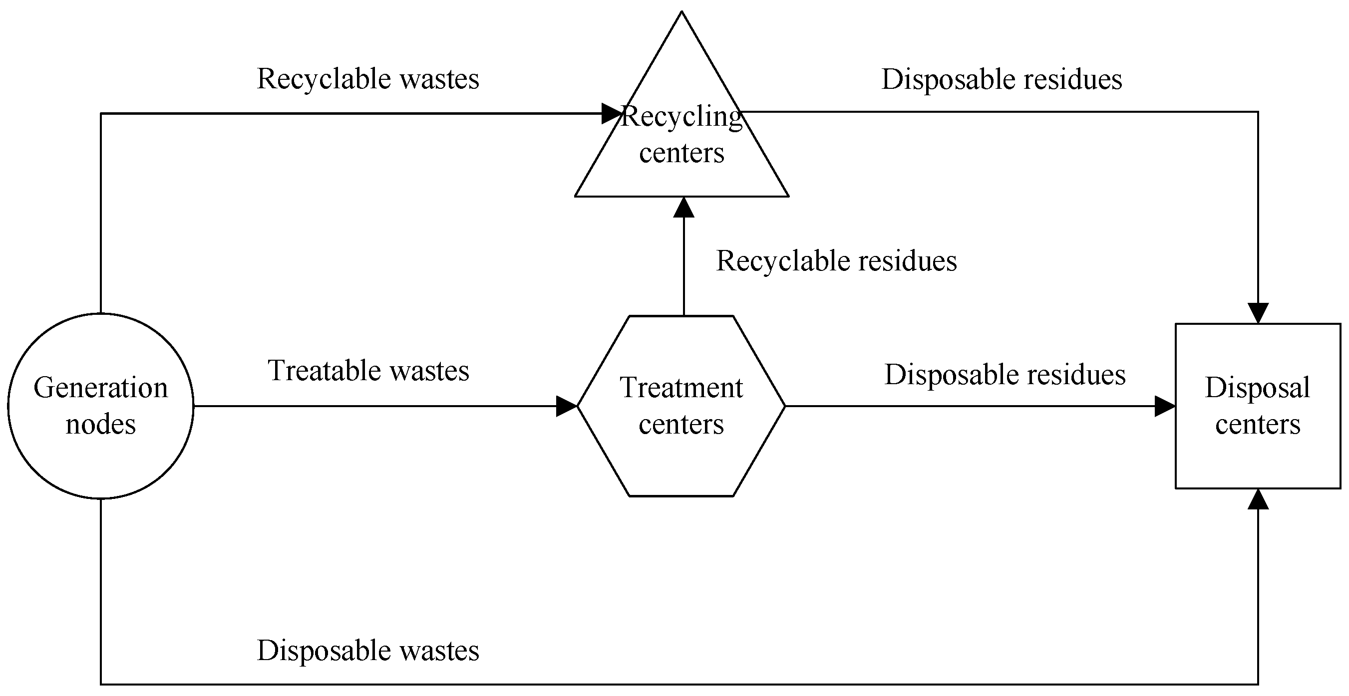
2. Problem Description
- Which existing recycling centers, treatment centers and disposal centers are closed.
- Which new recycling centers, treatment centers with which types of treatment technologies and disposal centers are opened.
- How to transport or allocate the recyclable, treatable and disposable hazardous wastes at generation nodes among recycling centers, treatment centers and disposal centers, respectively.
- How to transport or allocate the recyclable and disposable waste residues at treatment centers among recycling centers and disposal centers, respectively.
- How to transport or allocate the disposable waste residues at recycling centers among disposal centers.
- The planning horizon is discretized into a limited number of periods. The related cost, risk and capacity parameters in each period is deterministic. The cost in each period is uniformly discounted at the beginning of the planning horizon using a discount rate determined by the inflation rate divided by the nominal interest rate.
- The existing waste facilities remained from the last planning horizon are not included into the current planning horizon if they have no attractiveness in the aspects of capacity, cost and risk. Due to this selection, any existing waste facilities chosen into the current planning horizon must be operated by at least one period.
- Each existing waste facility can be closed at the end of a period. It cannot be reopened during the remaining of the planing horizon once it is closed at a period. If an existing waste facility is closed at the last period of the planning horizon, it means that this waste facility is operated in the whole planning horizon.
- Each new waste facility is opened at the beginning of a period. It cannot be closed during the remaining of the planing horizon once it is opened at a period.
3. Multi-Objective Model
3.1. Notations
3.2. Model Formulation
4. Augmented -Constraint Algorithm
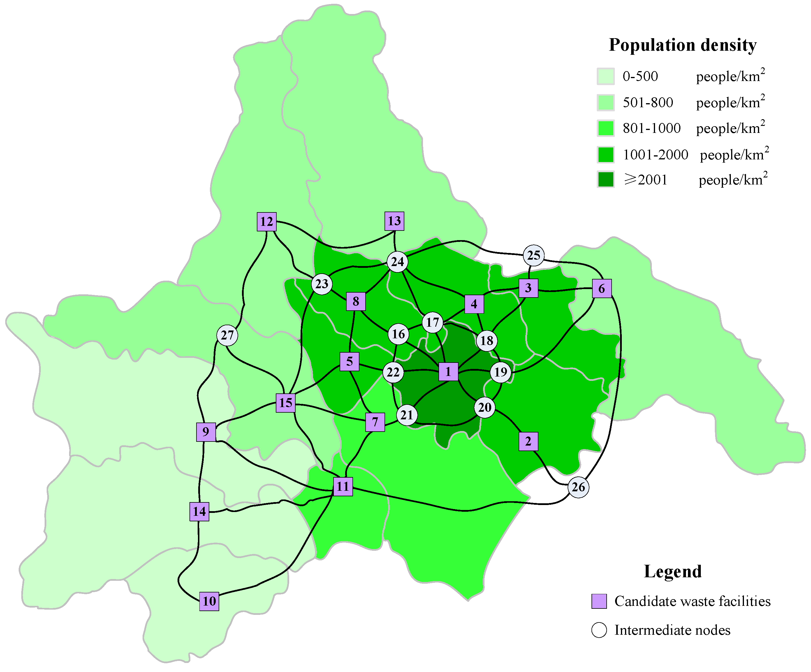
5. Case Study
5.1. Case Description and Parameter Setting
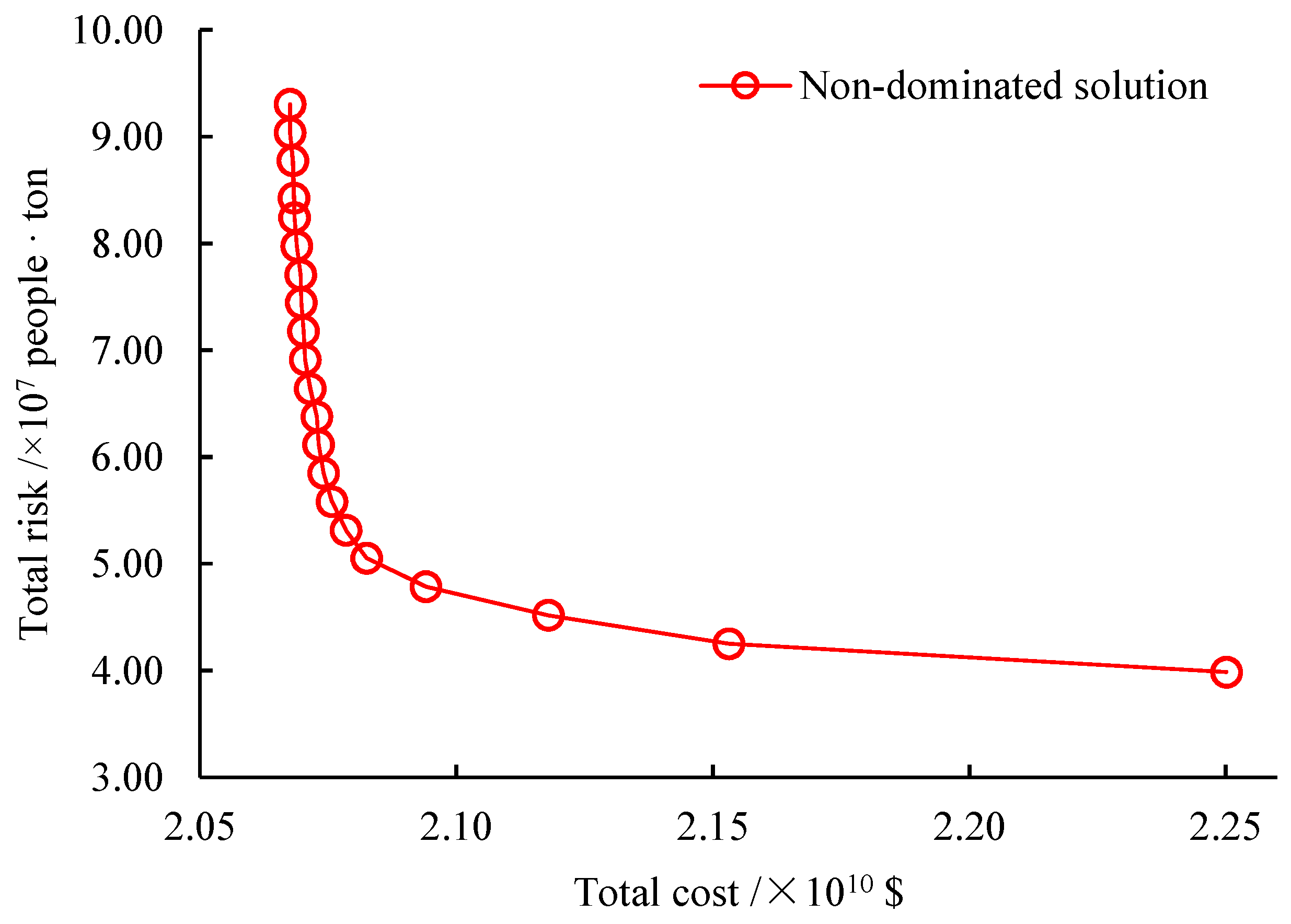
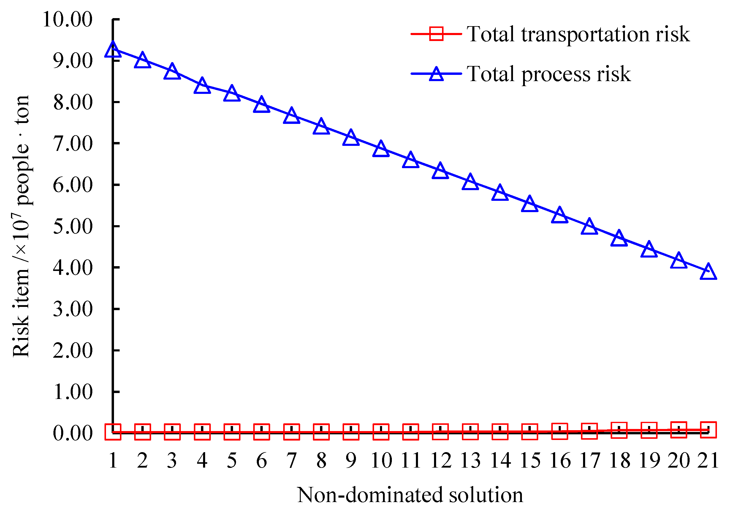
5.2. Computational Results
5.3. The Value of Multi-Period Optimization
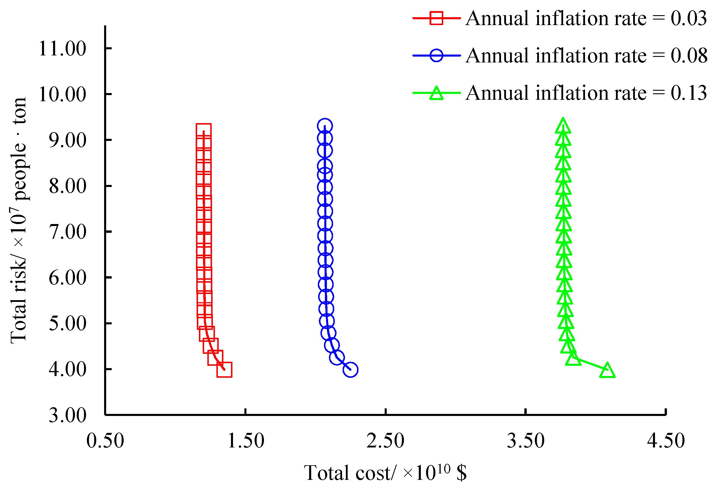
5.4. Sensitivity Analysis
6. Conclusions
Author Contributions
Funding
Acknowledgments
Conflicts of Interest
References
- Liu, W.; Xu, B. China Statistical Yearbook on Environment 2018; China Statistics Press: Beijing, China, 2019. [Google Scholar]
- Erkut, E.; Tjandra, S.A.; Verter, V. Chapter 9 hazardous materials transportation. In Transportation; Handbooks in Operations Research and Management Science; Barnhart, C., Laporte, G., Eds.; Elsevier: Amsterdam, The Netherlands, 2007; Volume 14, pp. 539–621. [Google Scholar]
- Zografros, K.G.; Samara, S. Combined location-routing model for hazardous waste transportation and disposal. Transp. Res. Record 1989, 1245, 52–59. [Google Scholar]
- ReVelle, C.; Cohon, J.; Shobrys, D. Simultaneous siting and routing in the disposal of hazardous wastes. Transp. Sci. 1991, 25, 138–145. [Google Scholar] [CrossRef]
- Stowers, C.L.; Palekar, U.S. Location models with routing considerations for a single obnoxious facility. Transp. Sci. 1993, 27, 350–362. [Google Scholar] [CrossRef]
- Wyman, M.M.; Kuby, M. Proactive optimization of toxic waste transportation, location and technology. Locat. Sci. 1995, 3, 167–185. [Google Scholar] [CrossRef]
- Boyer, O.; Sai Hong, T.; Pedram, A.; Mohd Yusuff, R.B.; Zulkifli, N. A mathematical model for the industrial hazardous waste location-routing problem. J. Appl. Math. 2013, 2013. [Google Scholar] [CrossRef]
- Jacobs, T.L.; Warmerdam, J.M. Simultaneous routing and siting for hazardous-waste operations. J. Urban Plan. Dev. 1994, 120, 115–131. [Google Scholar] [CrossRef]
- Current, J.; Ratick, S. A model to assess risk, equity and efficiency in facility location and transportation of hazardous materials. Locat. Sci. 1995, 3, 187–201. [Google Scholar] [CrossRef]
- Giannikos, I. A multiobjective programming model for locating treatment sites and routing hazardous wastes. Eur. J. Oper. Res. 1998, 104, 333–342. [Google Scholar] [CrossRef]
- Cappanera, P.; Gallo, G.; Maffioli, F. Discrete facility location and routing of obnoxious activities. Discret. Appl. Math. 2004, 133, 3–28. [Google Scholar] [CrossRef]
- List, G.; Mirchandani, P. An integrated network/planar multiobjective model for routing and siting for hazardous materials and wastes. Transp. Sci. 1991, 25, 146–156. [Google Scholar] [CrossRef]
- Alidi, A.S. An integer goal programming model for hazardous waste treatment and disposal. Appl. Math. Model. 1992, 16, 645–651. [Google Scholar] [CrossRef]
- Emek, E.; Kara, B.Y. Hazardous waste management problem: The case for incineration. Comput. Oper. Res. 2007, 34, 1424–1441. [Google Scholar] [CrossRef]
- Nema, A.K.; Gupta, S. Optimization of regional hazardous waste management systems: An improved formulation. Waste Manag. 1999, 19, 441–451. [Google Scholar] [CrossRef]
- Alumur, S.; Kara, B.Y. A new model for the hazardous waste location-routing problem. Comput. Oper. Res. 2007, 34, 1406–1423. [Google Scholar] [CrossRef]
- Samanlioglu, F. A multi-objective mathematical model for the industrial hazardous waste location-routing problem. Eur. J. Oper. Res. 2013, 226, 332–340. [Google Scholar] [CrossRef]
- Ghezavati, V.; Morakabatchian, S. Application of a fuzzy service level constraint for solving a multi-objective location-routing problem for the industrial hazardous wastes. J. Intell. Fuzzy Syst. 2015, 28, 2003–2013. [Google Scholar] [CrossRef]
- Yu, H.; Solvang, W.D. An improved multi-objective programming with augmented ε-constraint method for hazardous waste location-routing problems. Int. J. Environ. Res. Public Health 2016, 13, 548. [Google Scholar] [CrossRef]
- Zhao, J.; Huang, L.; Lee, D.H.; Peng, Q. Improved approaches to the network design problem in regional hazardous waste management systems. Transp. Res. Part E Logist. Transp. Rev. 2016, 88, 52–75. [Google Scholar] [CrossRef]
- Yilmaz, O.; Kara, B.Y.; Yetis, U. Hazardous waste management system design under population and environmental impact considerations. J. Environ. Manag. 2017, 203, 720–731. [Google Scholar] [CrossRef]
- Rabbani, M.; Danesh Shahraki, S.; Farrokhi-Asl, H.; Frederick, W.T.; Lim, S. A new multi-objective mathematical model for hazardous waste management considering social and environmental issues. Iran. J. Manag. Stud. 2018, 11, 831–865. [Google Scholar]
- Aydemir-Karadag, A. A profit-oriented mathematical model for hazardous waste locating- routing problem. J. Clean. Prod. 2018, 202, 213–225. [Google Scholar] [CrossRef]
- Zhao, J.; Verter, V. A bi-objective model for the used oil location-routing problem. Comput. Oper. Res. 2015, 62, 157–168. [Google Scholar] [CrossRef]
- Zhao, J.; Zhu, F. A multi-depot vehicle-routing model for the explosive waste recycling. Int. J. Prod. Res. 2016, 54, 550–563. [Google Scholar] [CrossRef]
- Zhao, J.; Ke, G.Y. Incorporating inventory risks in location-routing models for explosive waste management. Int. J. Prod. Econ. 2017, 193, 123–136. [Google Scholar] [CrossRef]
- Asgari, N.; Rajabi, M.; Jamshidi, M.; Khatami, M.; Farahani, R.Z. A memetic algorithm for a multi-objective obnoxious waste location-routing problem: A case study. Ann. Oper. Res. 2017, 250, 279–308. [Google Scholar] [CrossRef]
- Rabbani, M.; Heidari, R.; Farrokhi-Asl, H.; Rahimi, N. Using metaheuristic algorithms to solve a multi-objective industrial hazardous waste location-routing problem considering incompatible waste types. J. Clean. Prod. 2018, 170, 227–241. [Google Scholar] [CrossRef]
- Nickel, S.; da Gama, F.S. Multi-period facility location. In Location Science; Laporte, G., Nickel, S., Saldanha da Gama, F., Eds.; Springer International Publishing: Cham, Switzerland, 2015; pp. 289–310. [Google Scholar]
- Melachrinoudis, E.; Min, H.; Wu, X. A multiobjective model for the dynamic location of landfills. Locat. Sci. 1995, 3, 143–166. [Google Scholar] [CrossRef]
- Srivastava, A.K.; Nema, A.K. A multi-objective and multi-period location-allocation model for solid waste disposal facilities: A case study of Delhi, India. Int. J. Environ. Health 2008, 2, 184–197. [Google Scholar] [CrossRef]
- Nema, A.K.; Modak, P.M. A strategic design approach for optimization of regional hazardous waste management systems. Waste Manag. Res. 1998, 16, 210–224. [Google Scholar] [CrossRef]
- Najm, M.A.; El-Fadel, M.; Ayoub, G.; El-Taha, M.; Al-Awar, F. An optimisation model for regional integrated solid waste management I. Model formulation. Waste Manag. Res. 2002, 20, 37–45. [Google Scholar] [CrossRef]
- Najm, M.A.; El-Fadel, M.; Ayoub, G.; El-Taha, M.; Al-Awar, F. An optimisation model for regional integrated solid waste management II. Model application and sensitivity analyses. Waste Manag. Res. 2002, 20, 46–54. [Google Scholar] [CrossRef] [PubMed]
- Mitropoulos, P.; Giannikos, I.; Mitropoulos, I.; Adamides, E. Developing an integrated solid waste management system in western Greece: A dynamic location analysis. Int. Trans. Oper. Res. 2009, 16, 391–407. [Google Scholar] [CrossRef]
- LaGrega, M.D.; Buckingham, P.L.; Evans, J.C. Hazardous Waste Management, 2nd ed.; Waveland Press: Long Grove, IL, USA, 2010. [Google Scholar]
- Haimes, Y.Y.; Lasdon, L.S.; Wismer, D.A. On a bicriterion formulation of the problems of integrated system identification and system optimization. IEEE Trans. Syst. Man Cybern. 1971, SMC-1, 296–297. [Google Scholar]
- Mavrotas, G. Effective implementation of the ε-constraint method in multi-objective mathematical programming problems. Appl. Math. Comput. 2009, 213, 455–465. [Google Scholar] [CrossRef]
- Mavrotas, G.; Florios, K. An improved version of the augmented ε-constraint method (AUGMECON2) for finding the exact pareto set in multi-objective integer programming problems. Appl. Math. Comput. 2013, 219, 9652–9669. [Google Scholar] [CrossRef]


| Recycling Node | Recycling Rate | Fixed Opening Cost ( $) | Fixed Closing Cost ( $) | Fixed Operating Cost ( $/yr) | Variable Process Cost ($/t) | Lower Workload (t/yr) | Upper Capacity (t/yr) | Risk Consequence ( People) | Risk Probability () |
|---|---|---|---|---|---|---|---|---|---|
| 2–15 | 0.9 | 3000 | 150 | 200 | 300 | 5000 | 10,000 | [0.79,2.74] | 100 |
| Treatment | Treatment | Residue | Residue | Fixed | Fixed | Fixed | Variable | Lower | Upper | Risk | Risk |
|---|---|---|---|---|---|---|---|---|---|---|---|
| Node | Technology | Generation | Recyclable | Opening | Closing | Operating | Process | Workload | Capacity | Consequence | Probability |
| Rate | Rate | Cost | Cost | Cost | Cost | ||||||
| ( $) | ( $) | ( $/yr) | ($/t) | (t/yr) | (t/yr) | ( People) | () | ||||
| 2–15 | Solidification | 1.3 | 0.2 | 15,000 | 750 | 1000 | 600 | 5000 | 25,000 | [0.79,2.74] | 400 |
| 2–15 | Incineration | 0.2 | 0.0 | 30,000 | 1500 | 2000 | 1200 | 5000 | 25,000 | [0.79,2.74] | 600 |
| Disposal | Disposal | Fixed | Fixed | Fixed | Variable | Lower | Upper | Life | Risk | Risk |
|---|---|---|---|---|---|---|---|---|---|---|
| Node | Technology | Opening | Closing | Operating | Process | Workload | Capacity | Cycle | Consequence | Probability |
| Cost | Cost | Cost | Cost | Capacity | ||||||
| ( $) | ( $) | ( $/yr) | ($/t) | (t/yr) | (t/yr) | (t) | ( People) | () | ||
| 2–15 | Landfill | 27,000 | 13,500 | 1800 | 900 | 5000 | 30,000 | 600,000 | [0.79,2.74] | 200 |
| # | Total Cost | Total Risk | Computation Time |
|---|---|---|---|
| ($) | (People · ton) | (s) | |
| 1 | 20,676,026,329.8 | 93,053,886.4 | 6840.1 |
| 2 | 20,676,290,993.6 | 90,401,881.3 | 6480.2 |
| 3 | 20,680,992,688.7 | 87,742,662.8 | 6120.5 |
| 4 | 20,683,748,372.7 | 84,278,640.5 | 5760.2 |
| 5 | 20,684,303,588.8 | 82,424,225.8 | 5400.5 |
| 6 | 20,688,579,661.1 | 79,746,973.4 | 5040.1 |
| 7 | 20,697,031,567.1 | 77,105,788.8 | 4680.1 |
| 8 | 20,697,984,919.7 | 74,446,570.2 | 4321.1 |
| 9 | 20,701,497,158.4 | 71,787,351.7 | 3960.1 |
| 10 | 20,704,825,265.3 | 69,097,504.5 | 3600.1 |
| 11 | 20,712,097,631.4 | 66,441,114.6 | 3240.2 |
| 12 | 20,727,792,658.3 | 63,788,573.7 | 2880.1 |
| 13 | 20,731,113,889.2 | 61,150,477.7 | 2520.1 |
| 14 | 20,741,294,484.5 | 58,491,259.2 | 2160.9 |
| 15 | 20,757,661,992.1 | 55,832,040.7 | 1800.1 |
| 16 | 20,784,403,178.3 | 53,172,822.1 | 1440.1 |
| 17 | 20,825,111,380.6 | 50,513,603.6 | 1080.1 |
| 18 | 20,940,839,801.3 | 47,854,385.1 | 720.3 |
| 19 | 21,179,278,507.8 | 45,195,166.6 | 360.1 |
| 20 | 21,531,865,418.3 | 42,535,948.1 | 57.8 |
| 21 | 22,501,278,056.4 | 39,876,729.6 | 1.4 |
| Average | 3260.2 |
| # | Period | Recycling | Treatment | Treatment | Disposal | Total | Total |
|---|---|---|---|---|---|---|---|
| Centers | Centers | Centers | Centers | Cost | Risk | ||
| (Tech 1) | (Tech 2) | ($) | (People · ton) | ||||
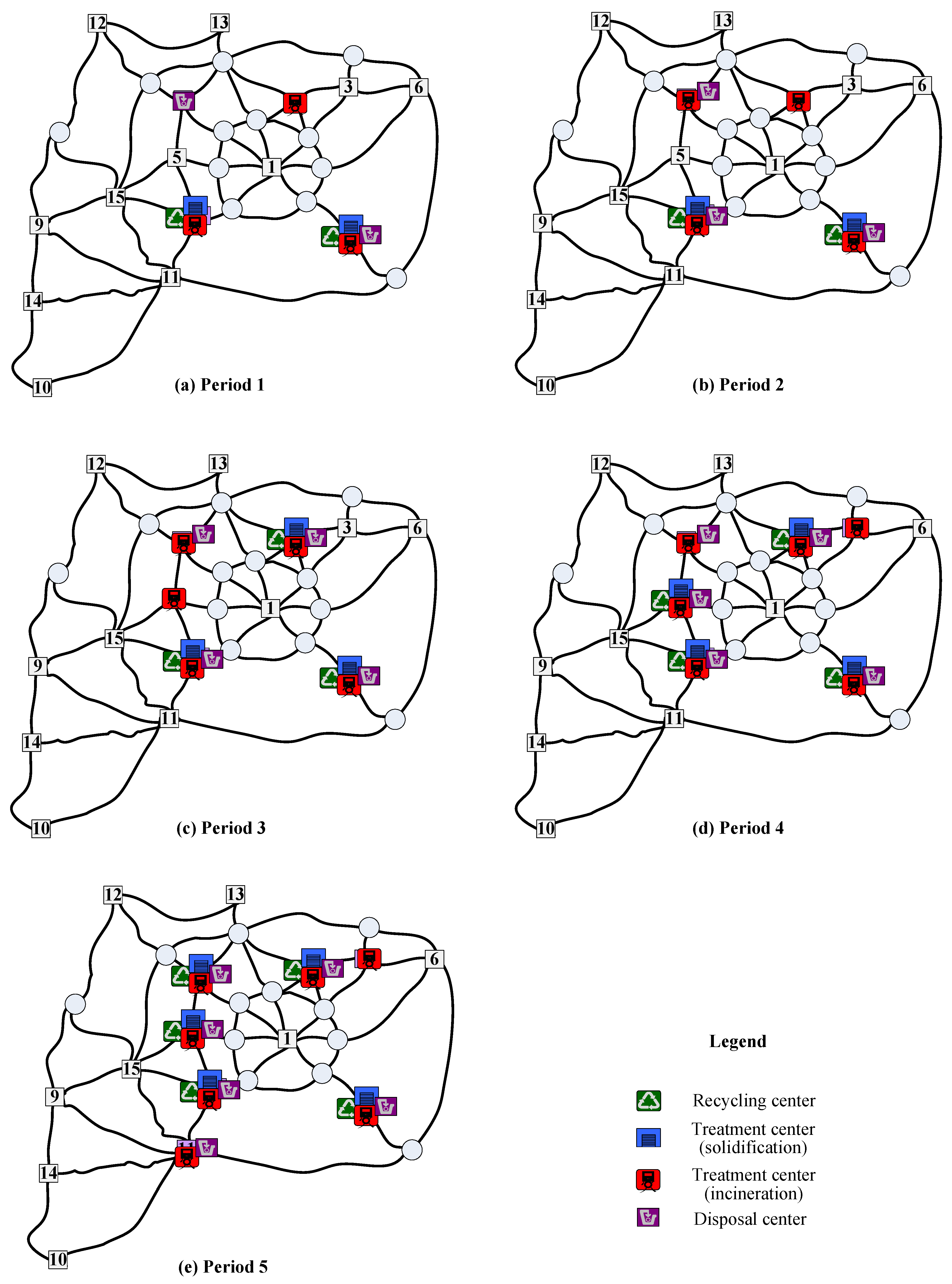
| 1 | 1 | 2,7 | 2,7 | 2,4,7 | 2,8 | 4,032,467,155.4 | 13,417,995.2 |
| 2 | 2,7 | 2,7 | 2,4,7,8 | 2,7,8 | 2,781,239,596.1 | 14,951,583.8 | |
| 3 | 2,4,7 | 2,4,7 | 2,4,5,7,8 | 2,4,7,8 | 3,557,848,264.7 | 18,733,069.8 | |
| 4 | 2,4,5,7 | 2,4,5,7 | 2,3,4,5,7 | 2,4,5,7,8 | 4,023,538,292.0 | 22,039,760.8 | |
| 8 | |||||||
| 5 | 2,4,5,7,8 | 2,4,5,7,8 | 2,3,4,5,7 | 2,4,5,7,8 | 6,280,933,021.5 | 23,911,476.8 | |
| 8,11 | 11 | ||||||
| Sum | 20,676,026,329.8 | 93,053,886.4 | |||||
| 2 | 1 | 2,9 | 2,9 | 2,7,13 | 2,9 | 4,034,422,517.5 | 9,433,350.4 |
| 2 | 2,9 | 2,9 | 2,3,7,13 | 2,9,13 | 2,788,936,065.9 | 10,428,807.1 | |
| 3 | 2,9,13 | 2,9,13 | 2,3,7,13,15 | 2,9,13,15 | 3,569,417,866.7 | 12,091,936.4 | |
| 4 | 2,3,9,13 | 2,3,9,13 | 2,3,7,8,13 | 2,3,9,13,15 | 4,032,625,809.9 | 15,804,776.6 | |
| 15 | |||||||
| 5 | 2,3,7,9,13 | 2,3,7,9,13 | 2,3,4,7,8 | 2,3,7,9,13 | 6,286,695,371.3 | 18,682,244.0 | |
| 13,15 | 15 | ||||||
| Sum | 20,712,097,631.4 | 66,441,114.6 | |||||
| 3 | 1 | 2,9 | 2,9,10 | 2,9,10,14 | 2,9,10 | 6,644,062,276.5 | 5,869,751.5 |
| 2 | 9,10 | 9,10 | 9,10,12,14 | 9,10,14 | 2,909,901,720.2 | 6,312,141.8 | |
| 3 | 9,10,14 | 9,10,14 | 9,10,12,13,14 | 9,10,12,14 | 3,625,857,963.5 | 7,738,874.6 | |
| 4 | 9,10,12,14 | 9,10,12,14 | 9,10,12,13,14 | 9,10,12,13,14 | 4,112,653,780.6 | 9,193,084.6 | |
| 15 | |||||||
| 5 | 9,10,12,13,14 | 9,10,12,13,14 | 9,10,12,13,14 | 6,9,10,12,13 | 5,208,802,315.6 | 10,762,877.0 | |
| 15 | 15 | 15 | 14,15 | ||||
| Sum | 22,501,278,056.4 | 39,876,729.6 |
| # | Period | Recycling | Treatment | Treatment | Disposal | Total | Total |
|---|---|---|---|---|---|---|---|
| Centers | Centers | Centers | Centers | Cost | Risk | ||
| (Tech 1) | (Tech 2) | ($) | (People · ton) | ||||
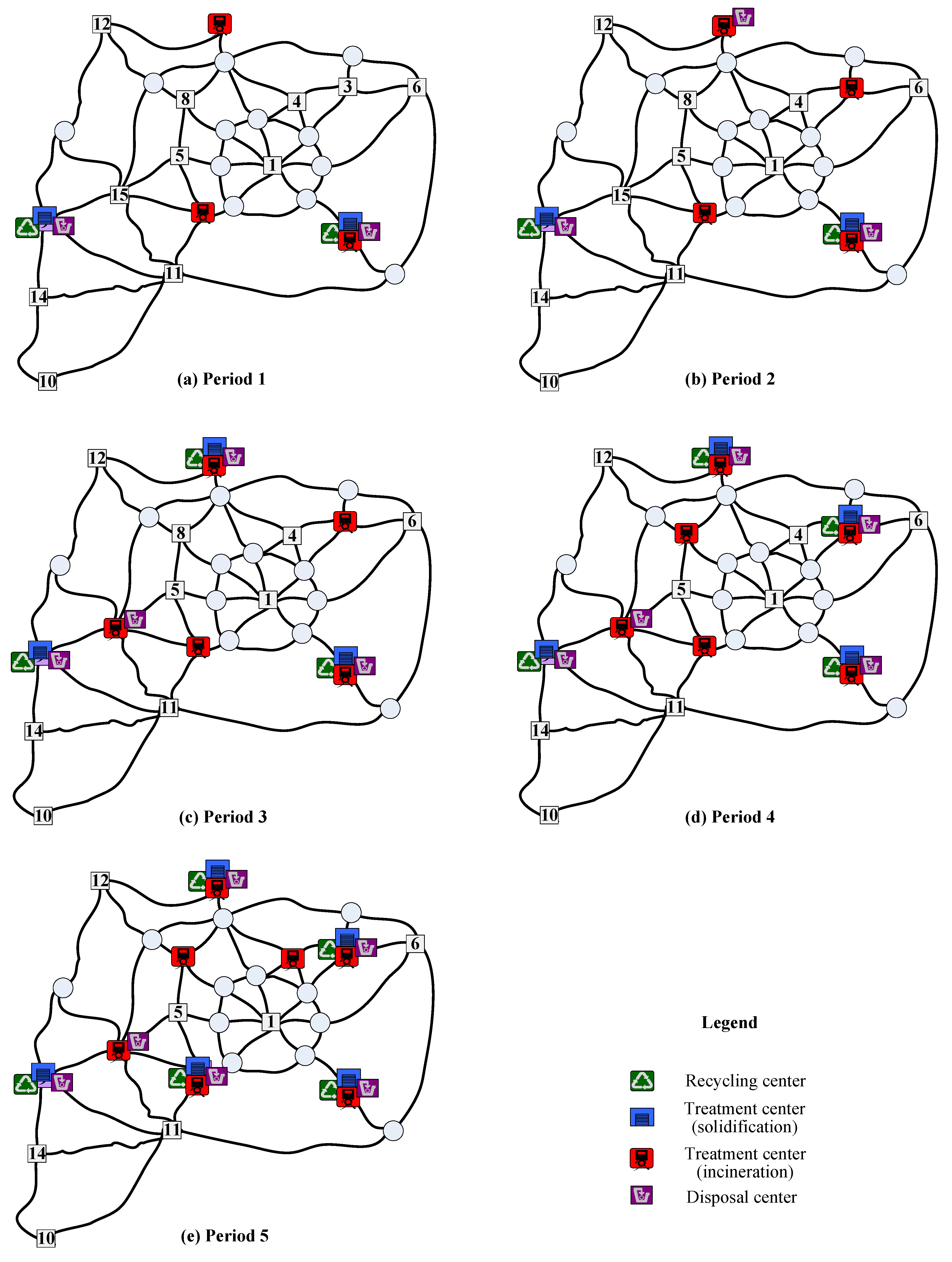
| 1 | 1 | 2,7 | 2,7 | 2,4,7 | 2,7 | 4,029,517,342.5 | 12,450,811.5 |
| 2 | 2,7 | 2,7 | 2,4,7,8 | 2,4,7 | 2,778,059,962.4 | 15,130,080.3 | |
| 3 | 2,4,7,8 | 2,4,7,8 | 2,4,7,8 | 2,4,7,8 | 3,292,300,142.7 | 19,482,053.2 | |
| 4 | 2,4,7,8 | 2,4,5,7,8 | 2,4,5,7,8 | 2,4,5,7,8 | 3,998,289,177.1 | 22,688,820.5 | |
| 5 | 2,4,7,8 | 2,4,5,7,8 | 2,3,4,5,7,8, | 2,3,4,5,7, | 7,578,642,683.3 | 23,195,257.7 | |
| 11,13 | 8,11 | ||||||
| Sum | 21,676,809,307.9 | 92,947,023.1 | |||||
| 2 | 1 | 2,15 | 2,15 | 2,13,15 | 2,15 | 4,034,817,674.7 | 9,777,504.4 |
| 2 | 2,15 | 2,15 | 2,9,13,15 | 2,9,15 | 2,789,513,985.0 | 10,198,248.5 | |
| 3 | 2,9,13,15 | 2,9,13,15 | 2,9,13,15 | 2,9,13,15 | 3,311,216,166.8 | 11,179,811.9 | |
| 4 | 2,9,13,15 | 2,9,12,13,15 | 2,9,12,13,15 | 2,9,12,13,15 | 4,622,778,191.0 | 12,391,553.1 | |
| 5 | 2,9,12,13,15 | 2,9,12,13,15 | 2,6,7,9,12, | 6,7,9,12,13, | 7,116,808,513.8 | 13,718,022.2 | |
| 13,15 | 14,15 | ||||||
| Sum | 21,875,134,531.4 | 57,265,140.2 | |||||
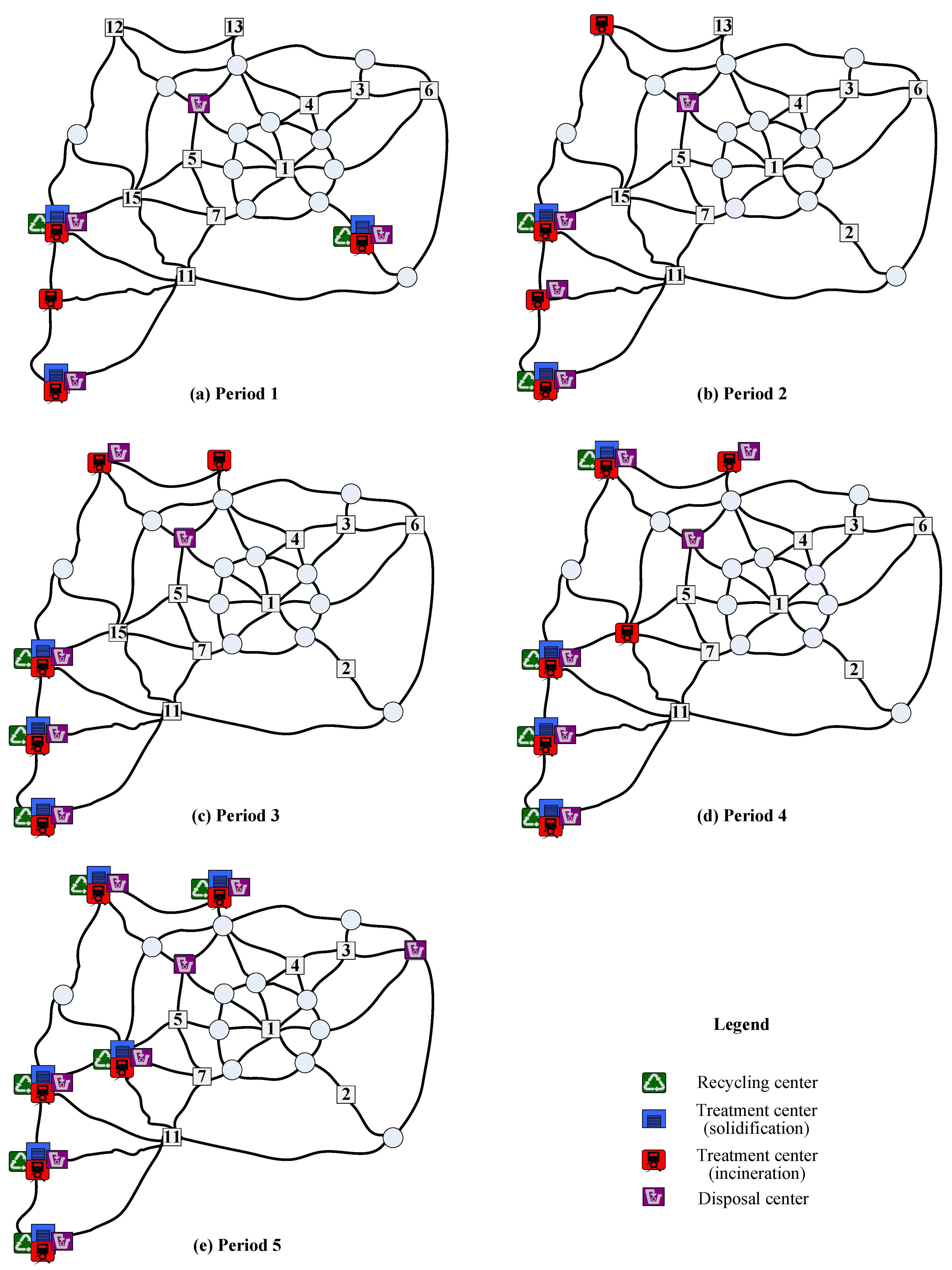
| 3 | 1 | 2,9,10 | 2,9,10 | 2,9,10 | 2,9,10,14 | 6,262,803,336.0 | 6,583,088.2 |
| 2 | 2,9,10 | 2,9,10,14 | 2,9,10,14 | 2,9,10,14 | 2,523,499,826.8 | 7,487,661.2 | |
| 3 | 2,9,10,14 | 2,9,10,12,14 | 2,9,10,12,14 | 2,9,10,12,14 | 3,682,431,946.3 | 8,675,022.0 | |
| 4 | 2,9,10,12,14 | 2,9,10,12,13, | 2,9,10,12,13, | 2,9,10,12,13, | 4,167,151,377.3 | 9,748,280.9 | |
| 14 | 14 | 14 | |||||
| 5 | 2,9,10,12,13, | 2,9,10,12,13, | 2,9,10,12,13, | 2,6,7,9,10,11, | 8,015,546,047.8 | 11,722,559.3 | |
| 14 | 14,15 | 14,15 | 12,13,14,15 | ||||
| Sum | 24,651,432,534.2 | 44,216,611.5 |
© 2019 by the authors. Licensee MDPI, Basel, Switzerland. This article is an open access article distributed under the terms and conditions of the Creative Commons Attribution (CC BY) license (http://creativecommons.org/licenses/by/4.0/).
Share and Cite
Zhao, J.; Huang, L. Multi-Period Network Design Problem in Regional Hazardous Waste Management Systems. Int. J. Environ. Res. Public Health 2019, 16, 2042. https://doi.org/10.3390/ijerph16112042
Zhao J, Huang L. Multi-Period Network Design Problem in Regional Hazardous Waste Management Systems. International Journal of Environmental Research and Public Health. 2019; 16(11):2042. https://doi.org/10.3390/ijerph16112042
Chicago/Turabian StyleZhao, Jun, and Lixiang Huang. 2019. "Multi-Period Network Design Problem in Regional Hazardous Waste Management Systems" International Journal of Environmental Research and Public Health 16, no. 11: 2042. https://doi.org/10.3390/ijerph16112042
APA StyleZhao, J., & Huang, L. (2019). Multi-Period Network Design Problem in Regional Hazardous Waste Management Systems. International Journal of Environmental Research and Public Health, 16(11), 2042. https://doi.org/10.3390/ijerph16112042