Predicted Mercury Soil Concentrations from a Kriging Approach for Improved Human Health Risk Assessment

 ,
,
Abstract
1. Introduction
2. Materials and Methods
2.1. Study Population
2.2. Collection of HBM-Data and Questionnaire Data
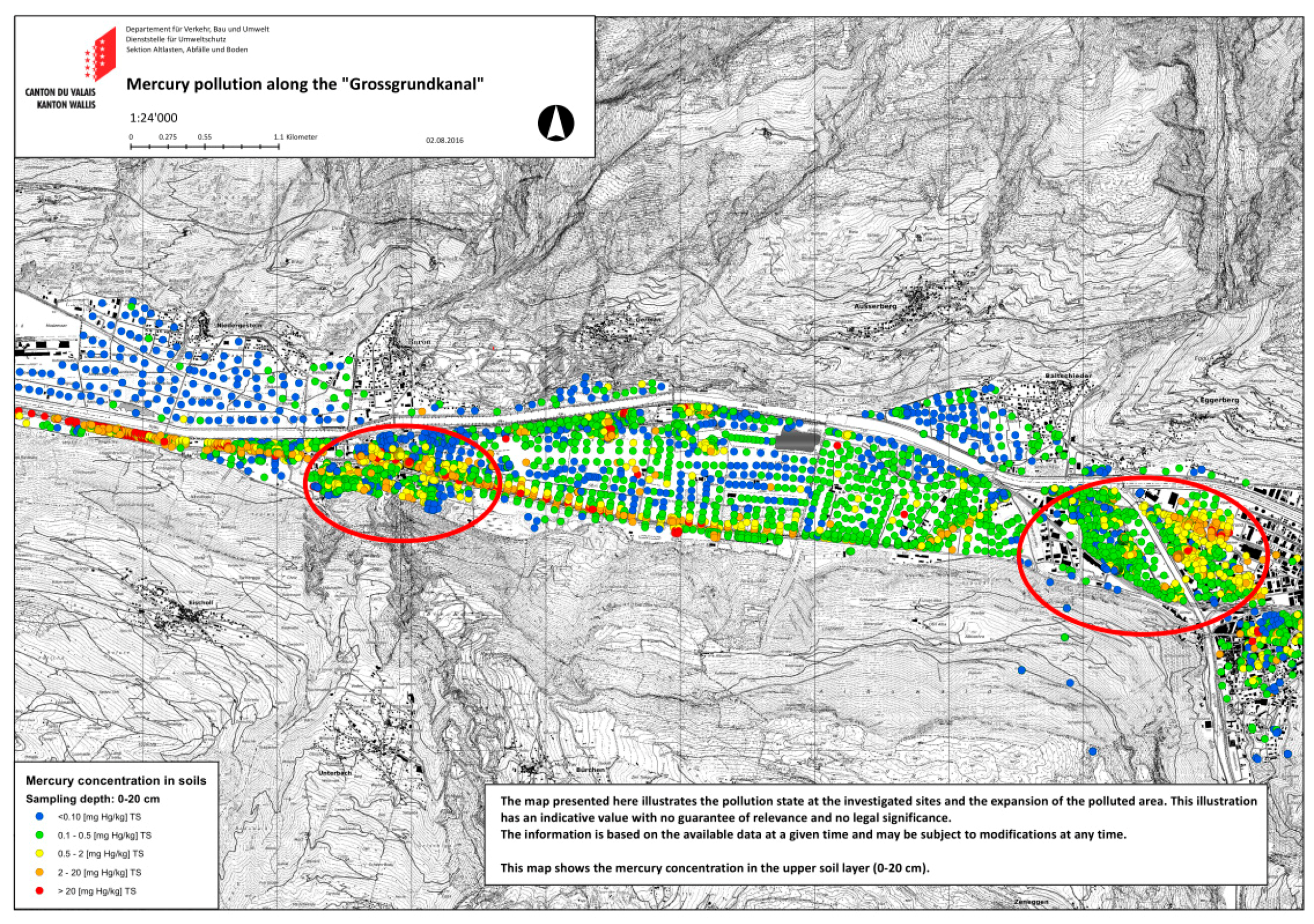
2.3. Study Site
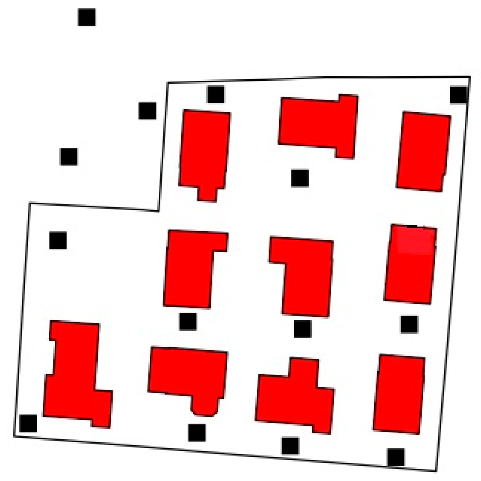
2.4. Soil Data
2.5. Distance to Canal
2.6. External Drift Kriging
2.7. Kriging-Induced Measurement Error
2.8. Explanatory Variables
2.9. Statistical Analyses
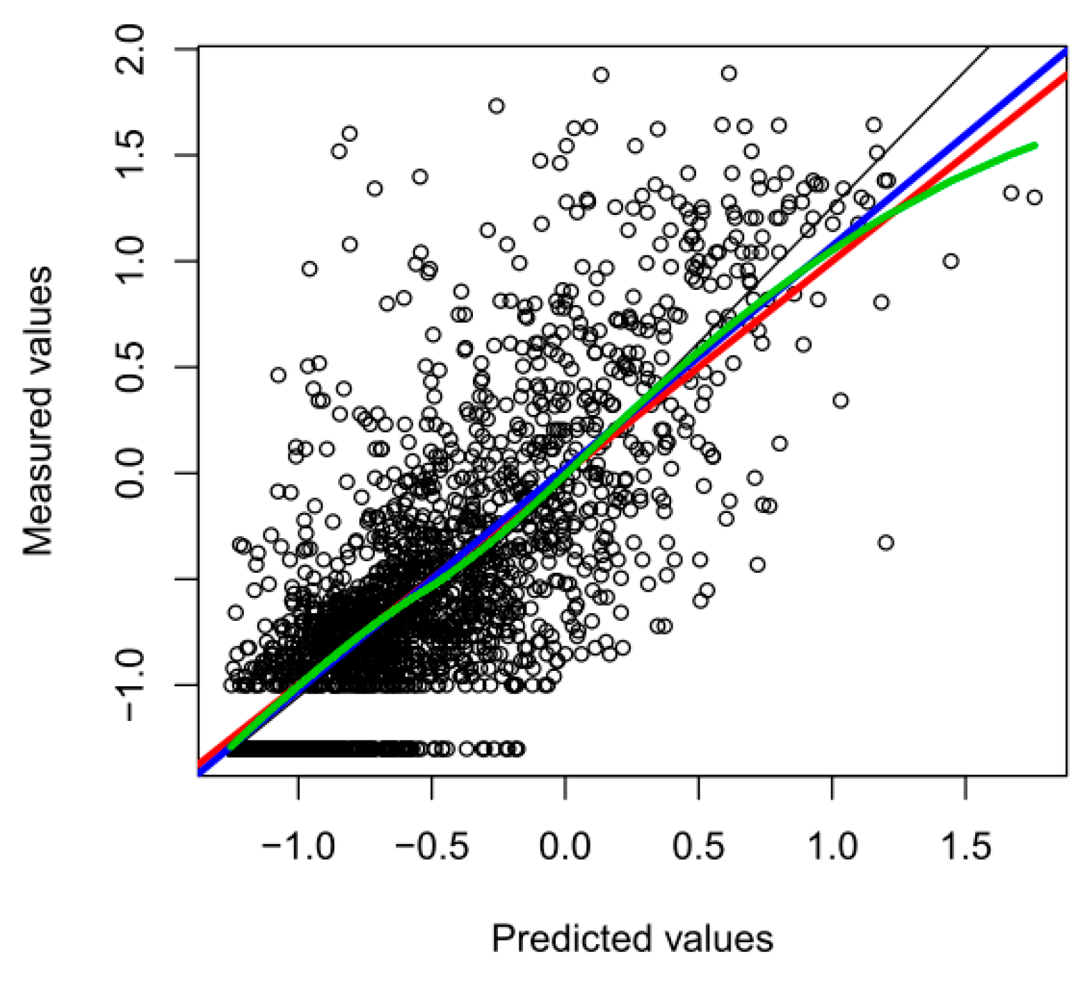
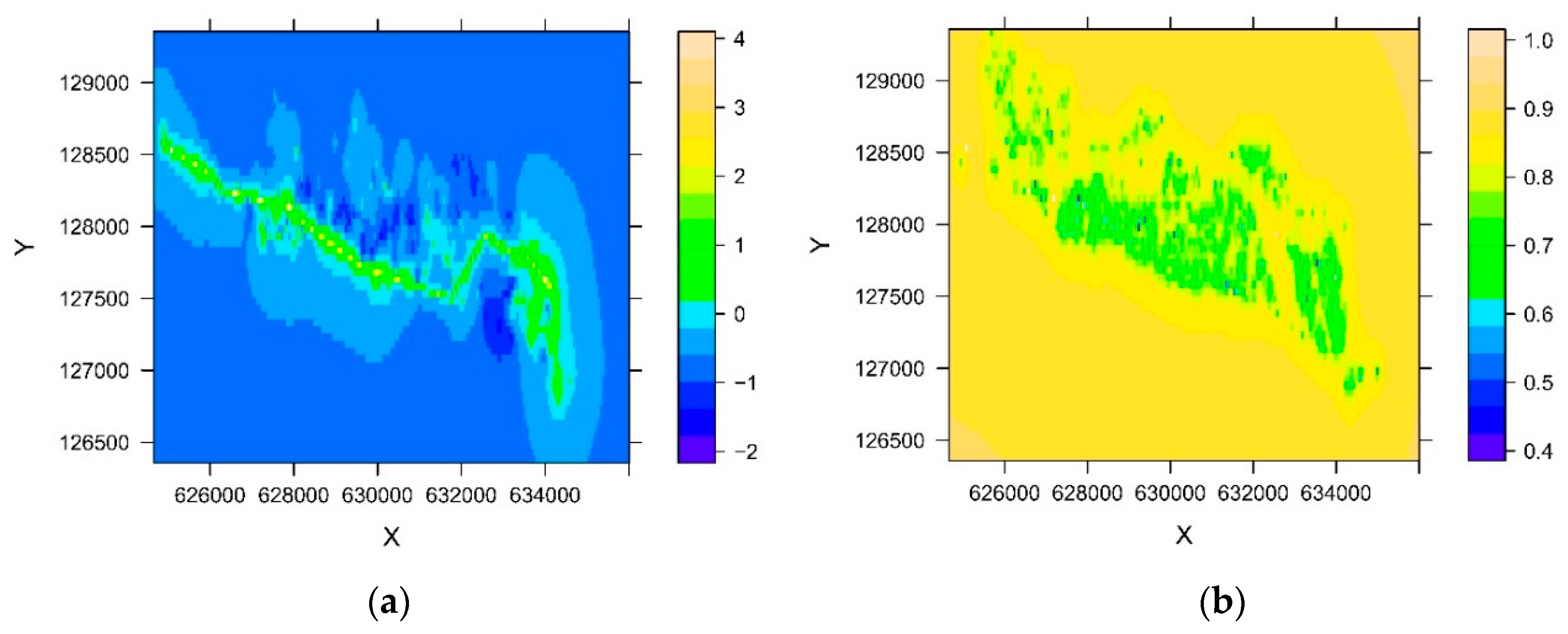
3. Results
4. Discussion
5. Conclusions
Author Contributions
Funding
Conflicts of Interest
References
- Molina, J.A.; Oyarzun, R.; Esbri, J.M.; Higueras, P. Mercury accumulation in soils and plants in the Almaden mining district, Spain: One of the most contaminated sites on Earth. Environ. Geochem. Health 2006, 28, 487–498. [Google Scholar] [CrossRef] [PubMed]
- Bailey, E.A.; Gray, J.E.; Theodorakos, P.M. Mercury in vegetation and soils at abandoned mercury mines in southwestern Alaska, USA. Geochem. Explor. Environ. Anal. 2002, 2, 275–285. [Google Scholar] [CrossRef]
- Biester, H.; Müller, G.; Schöler, H.F. Binding and mobility of mercury in soils contaminated by emissions from chlor-alkali plants. Sci. Total Environ. 2002, 284, 191–203. [Google Scholar] [CrossRef]
- Boszke, L.; Kowalski, A.; Astel, A.; Barański, A.; Gworek, B.; Siepak, J. Mercury mobility and bioavailability in soil from contaminated area. Environ. Geol. 2008, 55, 1075–1087. [Google Scholar] [CrossRef]
- Gray, J.E.; Crock, J.G.; Fey, D.L. Environmental geochemistry of abandoned mercury mines in West-Central Nevada, USA. Appl. Geochem. 2002, 17, 1069–1079. [Google Scholar] [CrossRef]
- Higueras, P.; Oyarzun, R.; Biester, H.; Lillo, J.; Lorenzo, S. A first insight into mercury distribution and speciation in soils from the Almadén mining district, Spain. J. Geochem. Explor. 2003, 80, 95–104. [Google Scholar] [CrossRef]
- Kocman, D.; Horvat, M.; Kotnik, J. Mercury fractionation in contaminated soils from the Idrija mercury mine region. J. Environ. Monit. 2004, 6, 696–703. [Google Scholar] [CrossRef] [PubMed]
- Reis, A.T.; Rodrigues, S.M.; Davidson, C.M.; Pereira, E.; Duarte, A.C. Extractability and mobility of mercury from agricultural soils surrounding industrial and mining contaminated areas. Chemosphere 2010, 81, 1369–1377. [Google Scholar] [CrossRef] [PubMed]
- Angerer, J.; Ewers, U.; Wilhelm, M. Human biomonitoring: State of the art. Int. J. Hyg. Environ. Health 2007, 210, 201–228. [Google Scholar] [CrossRef] [PubMed]
- Zhao, F.J.; McGrath, S.P.; Merrington, G. Estimates of ambient background concentrations of trace metals in soils for risk assessment. Environ. Pollut. 2007, 148, 221–229. [Google Scholar] [CrossRef] [PubMed]
- Imo, D.; Muff, S.; Schierl, R.; Byber, K.; Hitzke, C.; Bopp, M.; Bose-O’Reilly, S.; Held, L.; Dressel, H. Human-biomonitoring and Individual Soil Measurements for Children and Mothers in an area with recently detected mercury-contaminations and public health concerns: A Cross-sectional Study. Int. J. Environ. Health Res. 2018, in press. [Google Scholar]
- Hu, K.-L.; Zhang, F.-R.; Li, H.; Huang, F.; Li, B.-G. Spatial Patterns of Soil Heavy Metals in Urban-Rural Transition Zone of Beijing1 1Project supported by the National Natural Science Foundation of China (Nos. 40401025 and 49871005) and the Program for Changjiang Scholars and Innovative Research Team in University (No. IRT0412). Pedosphere 2006, 16, 690–698. [Google Scholar]
- Rodrigues, S.; Pereira, M.E.; Sarabando, L.; Lopes, L.; Cachada, A.; Duarte, A. Spatial distribution of total Hg in urban soils from an Atlantic coastal city (Aveiro, Portugal). Sci. Total Environ. 2006, 368, 40–46. [Google Scholar] [CrossRef] [PubMed]
- Marchant, B.P.; Tye, A.M.; Rawlins, B.G. The assessment of point-source and diffuse soil metal pollution using robust geostatistical methods: A case study in Swansea (Wales, UK). Eur. J. Soil Sci. 2011, 62, 346–358. [Google Scholar] [CrossRef]
- Núñez, O.; Fernández-Navarro, P.; Martín-Méndez, I.; Bel-Lan, A.; Locutura, J.F.; López-Abente, G. Arsenic and chromium topsoil levels and cancer mortality in Spain. Environ. Sci. Pollut. Res. Int. 2016, 23, 17664–17675. [Google Scholar] [CrossRef] [PubMed]
- Paul, R.; Cressie, N. Lognormal block kriging for contaminated soil. Eur. J. Soil Sci. 2011, 62, 337–345. [Google Scholar] [CrossRef]
- Saito, H.; Goovaerts, P. Accounting for source location and transport direction into geostatistical prediction of contaminants. Environ. Sci. Technol. 2001, 35, 4823–4829. [Google Scholar] [CrossRef] [PubMed]
- Cressie, N. Statistics for Spatial Data; John Wiley & Sons: New York, NY, USA, 1993. [Google Scholar]
- Carrat, F.; Valleron, A.-J. Epidemiologic Mapping using the “Kriging” Method: Application to an Influenza-like Epidemic in France. Am. J. Epidemiol. 1992, 135, 1293–1300. [Google Scholar] [CrossRef] [PubMed]
- Graham, A.J.; Atkinson, P.M.; Danson, F.M. Spatial analysis for epidemiology. Acta Trop. 2004, 91, 219–225. [Google Scholar] [CrossRef] [PubMed]
- Sampson, P.D.; Richards, M.; Szpiro, A.A.; Bergen, S.; Sheppard, L.; Larson, T.V.; Kaufman, J.D. A regionalized national universal kriging model using Partial Least Squares regression for estimating annual PM2.5 concentrations in epidemiology. Atmos. Environ. 2013, 75, 383–392. [Google Scholar] [CrossRef] [PubMed]
- Yang, W.; Wang, L. Spatial analysis and hazard assessment of mercury in soil around the coal-fired power plant: A case study from the city of Baoji, China. Environ. Geol. 2008, 53, 1381–1388. [Google Scholar] [CrossRef]
- Fang, F.; Wang, H.; Lin, Y. Spatial distribution, bioavailability, and health risk assessment of soil Hg in Wuhu urban area, China. Environ. Monit. Assess. 2011, 179, 255–265. [Google Scholar] [CrossRef] [PubMed]
- Ewers, U.; Boening, D.; Albrecht, J.; Radel, R.; Peter, G.; Uthoff, T. Risk assessment of soil contamination in a residential area: The importance and role of human biological monitoring—A case report. Gesundheitswesen 2004, 66, 536–544. [Google Scholar] [CrossRef] [PubMed]
- Gebel, T.; Behmke, C.; Dunkelberg, H. Influence of exposure to mercury, arsenic and antimony on body burden—A biomonitoring study. Zentralblatt fur Hygiene und Umweltmedizin Int. J. Hyg. Environ. Med. 1998, 201, 103–120. [Google Scholar]
- Safruk, A.M.; Berger, R.G.; Jackson, B.J.; Pinsent, C.; Hair, A.T.; Sigal, E.A. The bioaccessibility of soil-based mercury as determined by physiological based extraction tests and human biomonitoring in children. Sci. Total Environ. 2015, 518–519, 545–553. [Google Scholar] [CrossRef] [PubMed]
- World Health Organization. Biological Monitoring of Chemical Exposure in the Workplace–Guidelines; WHO: Geneva, Switzerland, 1996; Volume 1, p. 23. [Google Scholar]
- Cressie, N. The origins of kriging. Math. Geol. 1990, 22, 239–252. [Google Scholar] [CrossRef]
- Hengl, T.; Heuvelink, G.B.M.; Rossiter, D.G. About regression-kriging: From equations to case studies. Comput. Geosci. 2007, 33, 1301–1315. [Google Scholar] [CrossRef]
- Hofer, C.; Borer, F.; Bono, R.; Kayser, A.; Papritz, A. Predicting topsoil heavy metal content of parcels of land: An empirical validation of customary and constrained lognormal block kriging and conditional simulations. Geoderma 2013, 193, 200–212. [Google Scholar] [CrossRef]
- Papritz, A.; Herzig, C.; Borer, F.; Bono, R. Modelling the spatial distribution of copper in the soils around a metal smelter in northwestern Switzerland. Geostat. Environ. Appl. Proc. 2005, 343–354. [Google Scholar] [CrossRef]
- Papritz, A.; Schwierz, C. R-Package ‘Georob’. Robust Geostatistical Analysis of Spatial Data. 2017. Available online: https://cran.r-project.org/web/packages/georob/index.html (accessed on 16 April 2018).
- Gneiting, T. Correlation functions for atmospherical data analysis. Q. J. R. Meteorol. Soc. Part A 2007, 125, 2449–2464. [Google Scholar] [CrossRef]
- Kuensch, H.R.; Papritz, A.; Schwierz, C.; Stahel, W.A. Robust estimation of the external drift and the variogram of spatial data. In Proceedings of the ISI 58th World Statistics Congress of the International Statistical Institute, Dublin, Ireland, 21–26 August 2011. [Google Scholar]
- Matheron, G. Traité de Géostatistique Appliquée; Number 14 in Mem. Bur. Rech. Geog. Minieres; Editions Technip: Paris, France, 1962. [Google Scholar]
- Mazzella, A.; Mazzella, A. The Importance of the Model Choice for Experimental Semivariogram Modeling and Its Consequence in Evaluation Process. J. Eng. 2013, 2013. [Google Scholar] [CrossRef]
- Cleveland, W.S.; Grosse, E.; Shyu, W.M. Local regression models. Statistical Models in S. Wadsworth & Brooks/Cole; Springer: Berlin, Germany, 1992. [Google Scholar]
- Gryparis, A.; Paciorek, C.J.; Zeka, A.; Schwartz, J.; Coull, B.A. Measurement error caused by spatial misalignment in environmental epidemiology. Biostatistics (Oxf. Engl.) 2009, 10, 258–274. [Google Scholar] [CrossRef] [PubMed]
- Lopiano, K.K.; Young, L.J.; Gotway, C.A. Estimated generalized least squares in spatially misaligned regression models with Berkson error. Biostatistics (Oxf. Engl.) 2013, 14, 737–751. [Google Scholar] [CrossRef] [PubMed]
- Berkson, J. Are there Two Regressions? J. Am. Stat. Assoc. 1950, 45, 164–180. [Google Scholar] [CrossRef]
- Muff, S.; Riebler, A.; Held, L.; Rue, H.; Saner, P. Bayesian analysis of measurement error models using integrated nested Laplace approximations. J. R. Stat. Soc. Ser. C (Appl. Stat.) 2015, 64, 231–252. [Google Scholar] [CrossRef]
- R Core Team. R: A Language and Environment for Statistical Computing; R Foundation for Statistical Computing: Vienna, Austria, 2017; Available online: https://www.R-project.org/ (accessed on 16 April 2018).
- Bland, M. An Introduction to Medical Statistics, 4th ed.; Oxford University Press: Oxford, UK, 2015; p. 141. [Google Scholar]
- United Nations Environment Programme (UNEP); World Health Organization (WHO). Guidance for Identifying Populations at Risk from Mercury Exposure; WHO: Geneva, Switzerland, 2008. [Google Scholar]
- Albering, H.J.; van Leusen, S.M.; Moonen, E.J.; Hoogewerff, J.A.; Kleinjans, J.C. Human health risk assessment: A case study involving heavy metal soil contamination after the flooding of the river Meuse during the winter of 1993–1994. Environ. Health Perspect. 1999, 107, 37–43. [Google Scholar] [CrossRef] [PubMed]
- Cai, L.-M.; Xu, Z.-C.; Qi, J.-Y.; Feng, Z.-Z.; Xiang, T.-S. Assessment of exposure to heavy metals and health risks among residents near Tonglushan mine in Hubei, China. Chemosphere 2015, 127 (Suppl. C), 127–135. [Google Scholar] [CrossRef] [PubMed]
- Chabukdhara, M.; Nema, A.K. Heavy metals assessment in urban soil around industrial clusters in Ghaziabad, India: Probabilistic health risk approach. Ecotoxicol. Environ. Saf. 2013, 87 (Suppl. C), 57–64. [Google Scholar] [CrossRef] [PubMed]
- Khan, S.; Cao, Q.; Zheng, Y.M.; Huang, Y.Z.; Zhu, Y.G. Health risks of heavy metals in contaminated soils and food crops irrigated with wastewater in Beijing, China. Environ. Pollut. 2008, 152, 686–692. [Google Scholar] [CrossRef] [PubMed]
- Lai, H.-Y.; Hseu, Z.-Y.; Chen, T.-C.; Chen, B.-C.; Guo, H.-Y.; Chen, Z.-S. Health Risk-Based Assessment and Management of Heavy Metals-Contaminated Soil Sites in Taiwan. Int. J. Environ. Res. Public Health 2010, 7, 3595–3614. [Google Scholar] [CrossRef] [PubMed]
- Lim, H.-S.; Lee, J.-S.; Chon, H.-T.; Sager, M. Heavy metal contamination and health risk assessment in the vicinity of the abandoned Songcheon Au–Ag mine in Korea. J. Geochem. Explor. 2008, 96, 223–230. [Google Scholar] [CrossRef]
- Man, Y.B.; Sun, X.L.; Zhao, Y.G.; Lopez, B.N.; Chung, S.S.; Wu, S.C.; Cheung, K.C.; Wong, M.H. Health risk assessment of abandoned agricultural soils based on heavy metal contents in Hong Kong, the world’s most populated city. Environ. Int. 2010, 36, 570–576. [Google Scholar] [CrossRef] [PubMed]
- Manay, N.; Cousillas, A.Z.; Alvarez, C.; Heller, T. Lead contamination in Uruguay: The “La Teja” neighborhood case. Rev. Environ. Contam. Toxicol. 2008, 195, 93–115. [Google Scholar] [PubMed]
- Olawoyin, R.; Oyewole, S.A.; Grayson, R.L. Potential risk effect from elevated levels of soil heavy metals on human health in the Niger delta. Ecotoxicol. Environ. Saf. 2012, 85 (Suppl. C), 120–130. [Google Scholar] [CrossRef] [PubMed]
- Wcisło, E.; Ioven, D.; Kucharski, R.; Szdzuj, J. Human health risk assessment case study: An abandoned metal smelter site in Poland. Chemosphere 2002, 47, 507–515. [Google Scholar] [CrossRef]
- Aelion, C.M.; Davis, H.T.; Liu, Y.; Lawson, A.B.; McDermott, S. Validation of Bayesian kriging of arsenic, chromium, lead, and mercury surface soil concentrations based on internode sampling. Environ. Sci. Technol. 2009, 43, 4432–4438. [Google Scholar] [CrossRef] [PubMed]
- Journel, A.G. Nonparametric estimation of spatial distributions. Math. Geol. 1983, 15, 445. [Google Scholar] [CrossRef]
- Awata, H.; Linder, S.; Mitchell, L.E.; Delclos, G.L. Association of Dietary Intake and Biomarker Levels of Arsenic, Cadmium, Lead, and Mercury among Asian Populations in the U.S.: NHANES 2011–2012. Environ. Health Perspect. 2017, 125, 314–323. [Google Scholar] [PubMed]
- Awata, H.; Linder, S.; Mitchell, L.E.; Delclos, G.L. Biomarker Levels of Toxic Metals among Asian Populations in the U.S.: NHANES 2011–2012. Environ. Health Perspect. 2017, 125, 306–313. [Google Scholar] [PubMed]
- Muff, S.; Ott, M.; Braun, J.; Held, L. Bayesian two-component measurement error modelling for survival analysis using INLA—A case study on cardiovascular disease mortality in Switzerland. Comput. Stat. Data Anal. 2017, 113, 177–193. [Google Scholar] [CrossRef]
- Szpiro, A.A.; Paciorek, C.J. Measurement error in two-stage analyses, with application to air pollution epidemiology. Environmetrics 2013, 24, 501–517. [Google Scholar] [CrossRef] [PubMed]
- Szpiro, A.A.; Sheppard, L.; Lumley, T. Efficient measurement error correction with spatially misaligned data. Biostatistics (Oxf. Engl.) 2011, 12, 610–623. [Google Scholar] [CrossRef] [PubMed]
- Goovaerts, P. Geostatistics for Natural Resources Evaluation; Applied Geostatistics Series; Oxford University Press: New York, NY, USA, 1997. [Google Scholar]


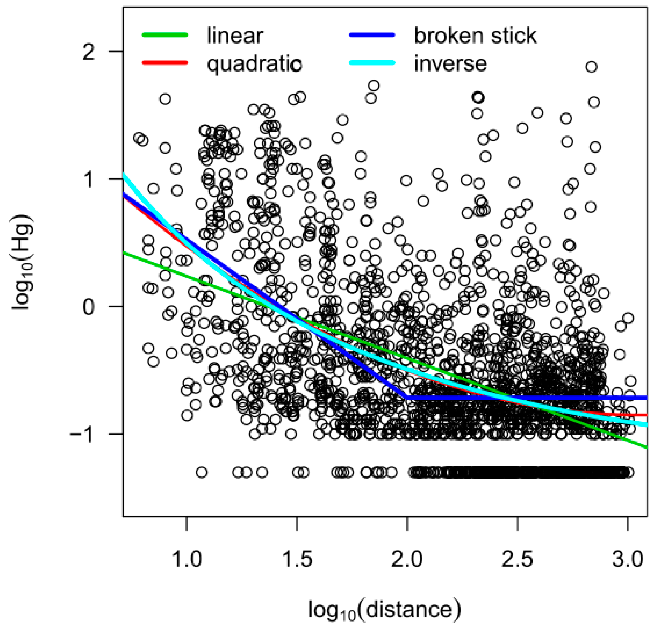
| Model | Coefficient | 95% CI | p-Value | AIC | BIC |
|---|---|---|---|---|---|
| Linear model | |||||
| logdist | −0.64 | −0.69 to −0.59 | <0.001 | 3435 | 3452 |
| Quadratic model | |||||
| logdist (logdist)2 | −1.91 0.31 | −2.29 to −1.54 0.22 to 0.40 | <0.001 <0.001 | 3393 | 3415 |
| Broken stick model | |||||
| logdist, bp | −1.24 | −1.33 to −1.15 | <0.001 | 3423 | 3439 |
| Inverse model | |||||
| logdist (1 + logdist)−1 | 0.16 6.90 | −0.10 to 0.42 4.72 to 9.08 | <0.001 <0.001 | 3399 | 3421 |
| Model Parameters | Estimates | 95% CI | p-Value |
|---|---|---|---|
| Intercept | 2.34 | 1.90 to 2.79 | <0.001 |
| log10 Hg | −2.23 | −2.72 to −1.73 | <0.001 |
| log10 Hg2 | 0.38 | 0.24 to 0.51 | <0.001 |
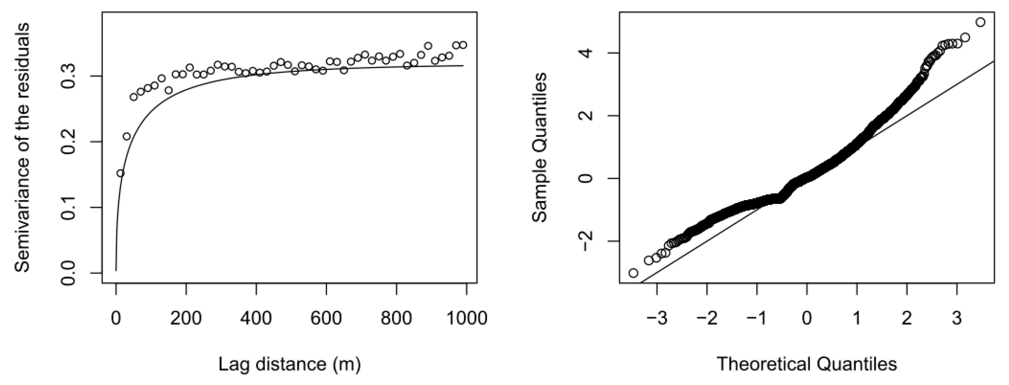
| Sill σ2 | 0.32 | ||
| Nugget-effect τ2 | 0.003 | ||
| Range parameter α | 46.67 |
| Variable | Coefficient | 95% CI | p-Value | Evidence for an Association |
|---|---|---|---|---|
| Amalgam fillings | 0.33 | 0.24 to 0.42 | <0.001 | Very strong evidence |
| Last time sea fish | 0.32 | 0.17 to 0.47 | <0.001 | |
| Age | −0.04 | −0.06 to −0.02 | <0.001 | |
| Interaction age × mother | 0.05 | 0.02, 0.08 | <0.001 | |
| Mother (indicator) | −0.97 | −1.64 to −0.31 | 0.004 | Strong evidence |
| Smoking | 0.30 | 0.09, 0.50 | 0.005 | |
| Sea fish | 0.08 | 0.03, 0.13 | 0.003 | |
| Log10 Hg soil | 0.02 | −0.06 to 0.10 | 0.64 | Little or no evidence |
| Determination limit | −0.08 | −0.25 to 0.09 | 0.37 | |
| Country of birth near the sea | −0.01 | −0.16 to 0.15 | 0.93 | |
| Eats vegetables from region | 0.07 | −0.03 to 0.18 | 0.18 |
| Variable | Coefficient | 95% CI | p-Value | Evidence for an Association |
|---|---|---|---|---|
| Amalgam fillings | 0.28 | 0.20 to 0.35 | <0.001 | Very strong evidence |
| Last time sea fish | 0.29 | 0.15 to 0.43 | <0.001 | |
| Age | −0.04 | −0.06 to −0.02 | <0.001 | |
| Mother (indicator) | −0.74 | −1.25 to −0.22 | 0.006 | Strong evidence |
| Smoking | 0.22 | 0.03 to 0.40 | 0.02 | Evidence |
| Sea fish | 0.06 | 0.01 to 0.11 | 0.04 | |
| Log10 Hg soil (predicted) Country of birth near the sea Eats vegetables from region Family variance σ2family Residual variance σ2ɛ | 0.08 0.03 0.01 0.03 0.06 | −0.23 to 0.42 −0.16 to 0.22 −0.11 to 0.13 0.01 to 0.06 0.04 to 0.07 | 0.61 0.78 0.81 | Little or no evidence |
| Variable | Coefficient | 95% CI | p-Value | Evidence for an Association |
|---|---|---|---|---|
| Sea fish | 0.17 | 0.11 to 0.22 | <0.001 | Very strong evidence |
| Country of birth near the sea | 0.19 | 0.01 to 0.37 | 0.041 | Evidence |
| Hair dyeing | −0.19 | −0.39 to 0.02 | 0.072 | Weak evidence |
| Mother (indicator) | −0.67 | −1.46 to 0.12 | 0.095 | |
| Log10 Hg soil (measured) | 0.05 | −0.05 to 0.14 | 0.32 | Little or no evidence |
| Determination limit | −0.02 | −0.22 to 0.17 | 0.81 | |
| Eats vegetables from region | 0.06 | −0.06 to 0.18 | 0.31 | |
| Smoking | 0.12 | −0.12 to 0.36 | 0.33 | |
| Amalgam fillings | 0.04 | −0.06 to 0.14 | 0.43 | |
| Age | 0.01 | −0.02 to 0.03 | 0.51 | |
| Interaction age × mother | 0.01 | −0.02 to 0.04 | 0.46 |
| Variable | Coefficient | 95% CI | p-Value | Evidence for an Association |
|---|---|---|---|---|
| Sea fish | 0.15 | 0.10 to 0.21 | <0.001 | Very strong evidence |
| Country of birth near the sea | 0.18 | −0.01 to 0.37 | 0.070 | Weak evidence |
| Hair dyeing | −0.15 | −0.34 to 0.05 | 0.15 | Little or no evidence |
| Mother (indicator) | −0.49 | −1.13 to 0.16 | 0.15 | |
| Log10 Hg soil (predicted) | 0.03 | −0.11 to 0.17 | 0.67 | |
| Eats vegetables from region | 0.06 | −0.06 to 0.18 | 0.33 | |
| Smoking | 0.07 | −0.16 to 0.30 | 0.54 | |
| Amalgam fillings | 0.03 | −0.06 to 0.13 | 0.51 | |
| Age | 0.01 | −0.02 to 0.03 | 0.33 | |
| Family variance σ2family | 0.01 | 0.01 to 0.04 | ||
| Residual variance σ2ɛ | 0.11 | 0.08 to 0.16 |
| Evidence for an Association | p-Value |
|---|---|
| Very strong evidence | <0.001 |
| Strong evidence | <0.01 |
| Evidence | Between 0.01 and 0.05 |
| Weak evidence | Between 0.05 and 0.1 |
| Little or no evidence | >0.1 |
© 2018 by the authors. Licensee MDPI, Basel, Switzerland. This article is an open access article distributed under the terms and conditions of the Creative Commons Attribution (CC BY) license (http://creativecommons.org/licenses/by/4.0/).
Share and Cite
Imo, D.; Dressel, H.; Byber, K.; Hitzke, C.; Bopp, M.; Maggi, M.; Bose-O’Reilly, S.; Held, L.; Muff, S. Predicted Mercury Soil Concentrations from a Kriging Approach for Improved Human Health Risk Assessment. Int. J. Environ. Res. Public Health 2018, 15, 1326. https://doi.org/10.3390/ijerph15071326
Imo D, Dressel H, Byber K, Hitzke C, Bopp M, Maggi M, Bose-O’Reilly S, Held L, Muff S. Predicted Mercury Soil Concentrations from a Kriging Approach for Improved Human Health Risk Assessment. International Journal of Environmental Research and Public Health. 2018; 15(7):1326. https://doi.org/10.3390/ijerph15071326
Chicago/Turabian StyleImo, David, Holger Dressel, Katarzyna Byber, Christine Hitzke, Matthias Bopp, Marion Maggi, Stephan Bose-O’Reilly, Leonhard Held, and Stefanie Muff. 2018. "Predicted Mercury Soil Concentrations from a Kriging Approach for Improved Human Health Risk Assessment" International Journal of Environmental Research and Public Health 15, no. 7: 1326. https://doi.org/10.3390/ijerph15071326
APA StyleImo, D., Dressel, H., Byber, K., Hitzke, C., Bopp, M., Maggi, M., Bose-O’Reilly, S., Held, L., & Muff, S. (2018). Predicted Mercury Soil Concentrations from a Kriging Approach for Improved Human Health Risk Assessment. International Journal of Environmental Research and Public Health, 15(7), 1326. https://doi.org/10.3390/ijerph15071326