4.2.2. Spatial Panel Data Results
We will now turn to the spatial econometric analysis.
Table 4 and
Table 5 report the estimated results of the SDM model that controls for both spatial and time effects. Two fields (fixed effects estimates and random effects estimates) with triple columns contain these results in each table. In
Table 4, the three columns in each field list and compare the results of three model specifications: the model with a cubic term of GDP (M1), the model with a quadratic term of GPD (M2), and the model with a linear term of GDP (M3). In a similar way,
Table 5 compares the estimated results of the three models incorporating urbanization’s cubic, quadratic, and linear terms.
As shown in
Table 4 and
Table 5, Hausman tests (against fixed effects) under the three model specifications all reject the null hypothesis: the unobserved individual effects in the provinces are not correlated with the independent variables in the models. Thus, we only focus on the results of the GDP–nitrogen oxides and urbanization–nitrogen oxides models with two-way fixed effects in the following discussion.
When including two-way fixed effects in M1 and M2, all the Chi-square statistics of all LR and Wald tests of the GDP–nitrogen oxides and urbanization–nitrogen oxides models reject both hypotheses,
H0:
and
H0:
. In other words: the SDM cannot be simplified to either the SLM or the SEM if one of the polynomial models is adopted. On the other hand, the Wald and LR tests in M3 (
Table 4 and
Table 5) do not reject their null hypothesis.
It is noteworthy that the coefficients’ estimates in the non-spatial model indicate the marginal effects of the driving forces (population and energy intensity) on the dependent variable (nitrogen oxides emissions), whereas the parameters’ estimates in the SDM or SLM do not. Instead, the independent variables’ direct and indirect (spillover) effects on the SDM need to be calculated by Equation (13), and the estimate results are reported in
Table 6 and
Table 7. Equation (13) is derived from Equation (14), and Equation (14) from Equation (6). The reciprocal term
is calculated by Equation (15). All the parameters that need to be brought into Equations (13) and (15) are already estimated and reported in
Table 4 and
Table 5. The diagonal elements of the partial derivatives matrix in Equation (13) indicates the direct effects (elasticity) of the kth explanatory variable, and all the off-diagonal elements refer to its spillover effects. Consequently, if
and
, then spillover effects do not exist. The difference between the driving forces’ direct effects and their estimated coefficients is due to the feedback effects that travel through adjacent provinces and then back to the provinces themselves. The feedback effects consist of two parts: the value of the spatially lagged dependent variable (W*ln NOx) and the coefficients of the spatially lagged explanatory variables (population and energy intensity). Some prior EKC studies that applied the spatial econometric approaches either mistakenly reported the coefficient estimates as the direct and spillover effects, or avoided to report these effects in the SDM/SLM [
18,
20,
36].
Another issue that has never been correctly discussed is the calculation of the turning points in the environmental Kuznets curve estimated by the SDM/SLM. Kang, Zhao, and Yang [
26] applied a spatial econometric approach and found an inverse N-shaped CO
2 EKC in China. However, they derived the turning points directly from the estimates of the GDP coefficients, which is invalid. The same problem occurred in Zhou, Ye, and Ge’s [
19] study. In most situations, the EKC function is smooth, thus the limit points of the EKC function are the turning points. As for the SDM, its right-hand side contains the dependent variable, thus one needs to first derive the Equations (6)–(14) and then let the first-order derivative to be zero, so that the parameters for calculating EKC’s turning points can be obtained (here, we assume the EKC as a single variable function, since the EKC hypothesis solely focuses on the affluence’s impact). Thus, we argue that, when fitting the EKC by the SDM, one needs to apply the direct effects estimated through Equation (14), instead of using parameter estimates of the spatially lagged variable, to calculate the turning points.
Table 6 and
Table 7 report the direct and spillover effects estimated according to
Table 4 and
Table 5 (fixed effects estimates). Model 1 (M1), Model 2 (M2), and Model 3 (M3) are respectively the GDP–nitrogen oxides/urbanization–nitrogen oxides models with cubic, quadratic, and linear terms of GDP/urbanization.
Turning our attention to the GDP–nitrogen oxides model results, the cubic, quadratic, and linear terms of the GDP’s coefficient (
Table 4, M1) and direct effects (
Table 6, M1) are statistically significant at a 5% level. Besides, the greater adjusted R
2 and log likelihood (
Table 4, M1) of the cubic model suggests that Model 1 (
Table 6) fits the data better than Models 2 and 3 (
Table 6). The significant effect estimates of energy intensity have the expected signs in Model 1. As we mentioned in
Section 4.2.2, if we adopt the polynomial model, the SDM should not be simplified to the SLM or SEM. Therefore, the cubic form of the GDP–nitrogen oxides model is the appropriate specification for empirical analysis (the linear and quadratic models are inherently nested in the cubic model, therefor the cubic model should be adopted when parameters of linear and polynomial terms are significant at the same time).
This finding shows that the estimated direct and spillover effects (elasticity) of energy intensity are highly significant at the 1% and 10% level respectively, and their signs are positive as expected. The effect of 1% growth in local energy intensity will lead to an increase in local nitrogen oxides emissions by 0.297%, other conditions being constant. LeSage and Pace [
37] pointed out that the spillover effects are defined as the impact that a specific region exerts on all adjacent regions or vice versa. Thus, the impact of a 1% growth in local energy intensity will, on average, cause a 0.375% increase in nitrogen oxides emissions in neighboring provinces, all else being equal. On the other hand, both the direct and the spillover effects of the population are not significantly different from zero, which implies that a specific province’s population barely affects local and other provinces’ emissions. The highly significant linear, quadratic, and cubic terms of GDP per capita (
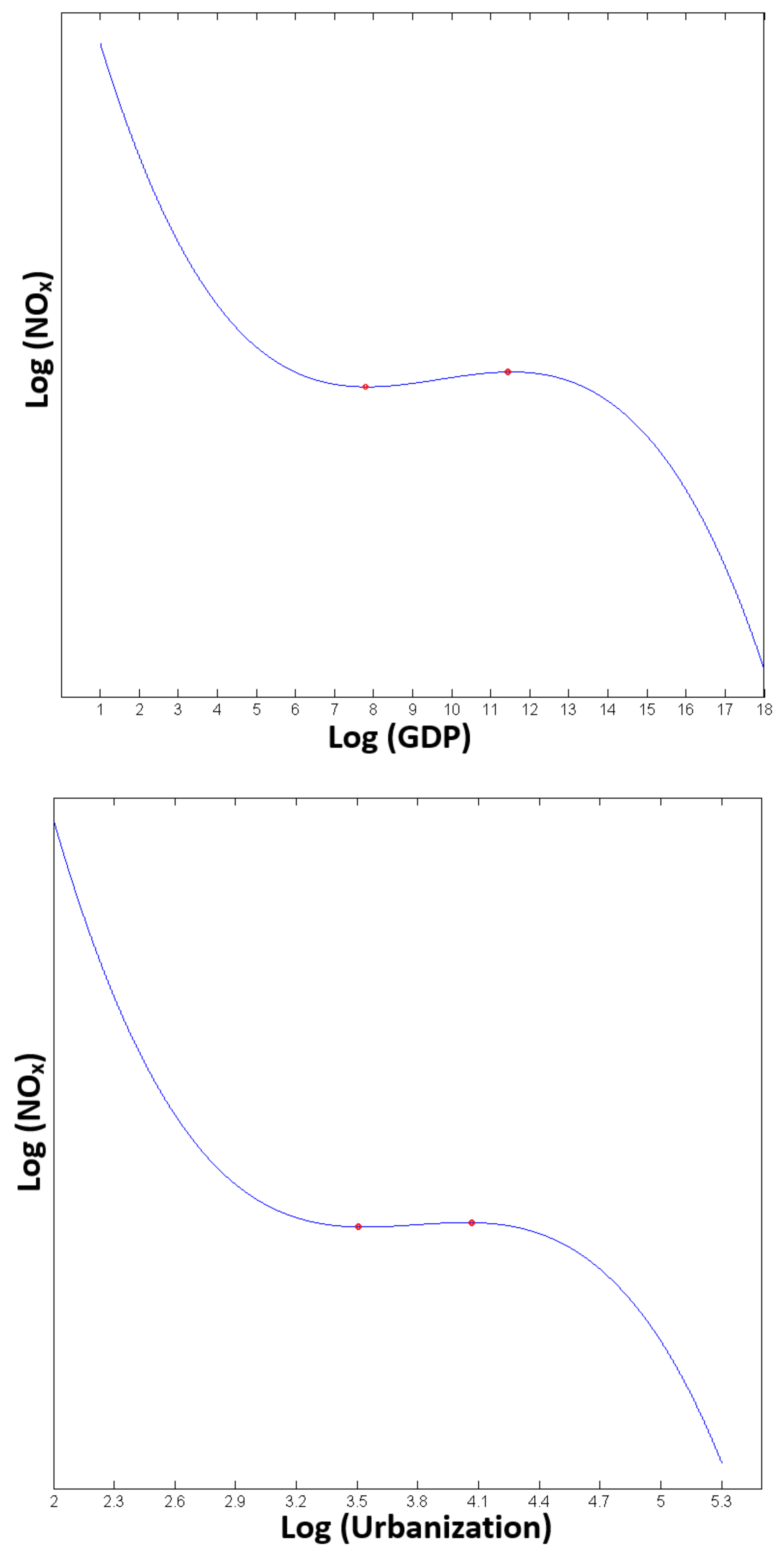
Table 6, M1) point to an inversely N-shaped EKC for the nexus between NO
x emission and economic growth (
Figure 2), which is consistent with the findings in prior China’s CO
2 and SO
2 EKC studies [
19,
20,
26]. Moreover, two turning points of the inverse N-shaped trajectory are approximately 2551 Renminbi (RMB) and 102,775 RMB, respectively (these two turning points are estimated on the basis of the polynomial equation
). Based on our sample, most of the economically developing provinces/cities (e.g., Guangxi, Xinjiang, and Qinghai provinces) are in the upward phase after the first turning point. There exists a general uptrend in nitrogen oxides emissions in such areas, and the personal incomes in the areas are between these two turning points. On the contrary, several developed cities with GDP per capita over 102,775 RMB (Beijing, Tianjin, and Shanghai) are experiencing a persisting decline in nitrogen oxides emissions. None of the observed per capita GDP is below 2551 RMB. The lowest one is 8237 RMB, in Guizhou province in 2010.
We will now turn to the Urbanization–nitrogen oxides model results. Similar to the GDP-nitrogen oxides model outcomes, all the polynomial terms of the urbanization’s coefficient (
Table 5, M1) and direct effects (
Table 7, M1) are statistically significant. Besides, the greater adjusted R
2 and log likelihood (
Table 5, M1) of the cubic model suggest that this model has the best explanatory power. Other than that, the energy intensity estimates remain positive, significant, and almost unchanged (0.240 and 0.355). Statistically, the population’s direct and spillover effects on emission are still not different from zero. Thus, the cubic Urbanization–nitrogen oxides model results are consistent with the cubic GDP–nitrogen oxides model results.
Because of the significant linear and polynomial terms of urbanization (
Table 7, M1), we infer that there exists an inversely N-shaped EKC for the Urbanization–nitrogen oxides nexus (
Figure 2), which is somewhat different from a prior study of China’s urbanization and industrial pollution [
38]. This is probably because this prior study did not apply the EKC model as the theoretical foundation for its empirical analysis and applied different pollution indicators. Two turning points of the inverse N-shape trajectory are approximately 34.56% and 56.67%, respectively (these two turning points are estimated on the basis of the polynomial equation
). In our sample, the urbanization levels of Beijing, Tianjin, Shanghai, and Guangdong and Jiangsu provinces are already over 56.67% at the beginning, and their local nitrogen oxides emissions indeed experienced downward trends as urbanization proceeded in the whole study period. Conversely, emissions in the rest of the provinces in the sample firstly experienced upward trends and then declined after approximately reaching 56.67%.
Unlike the population term, the autoregressive parameters of W log NO
x in the SDM (
Table 4 and
Table 5) are positive and statistically significant at the 1% level, which further testifies and demonstrates the spillover effects of nitrogen oxides emissions among the neighboring provinces. Specifically, a 1% increase and decrease of local nitrogen oxides emissions would lead to about a 0.3% corresponding variation in neighboring provinces and vice versa.


