Evaluation of Sources and Patterns of Elemental Composition of PM2.5 at Three Low-Income Neighborhood Schools and Residences in Quito, Ecuador

 ,
, 
Abstract
1. Introduction
2. Materials and Methods
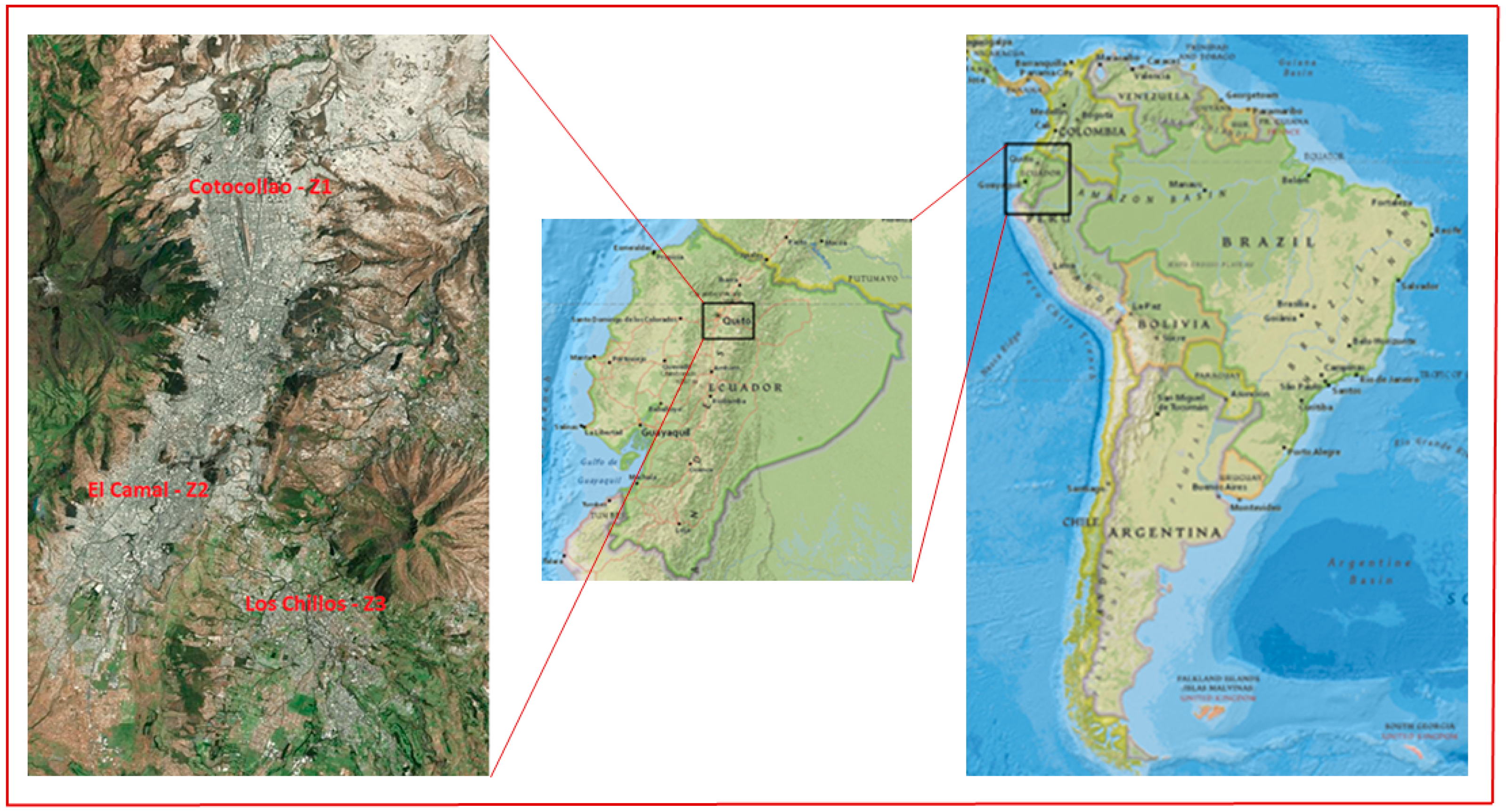
2.1. Study Sites and Meteorology
2.2. Sampling Plan
2.3. PM2.5 Gravitational and Elemental Analysis
2.4. Statistical Data Analysis
3. Results
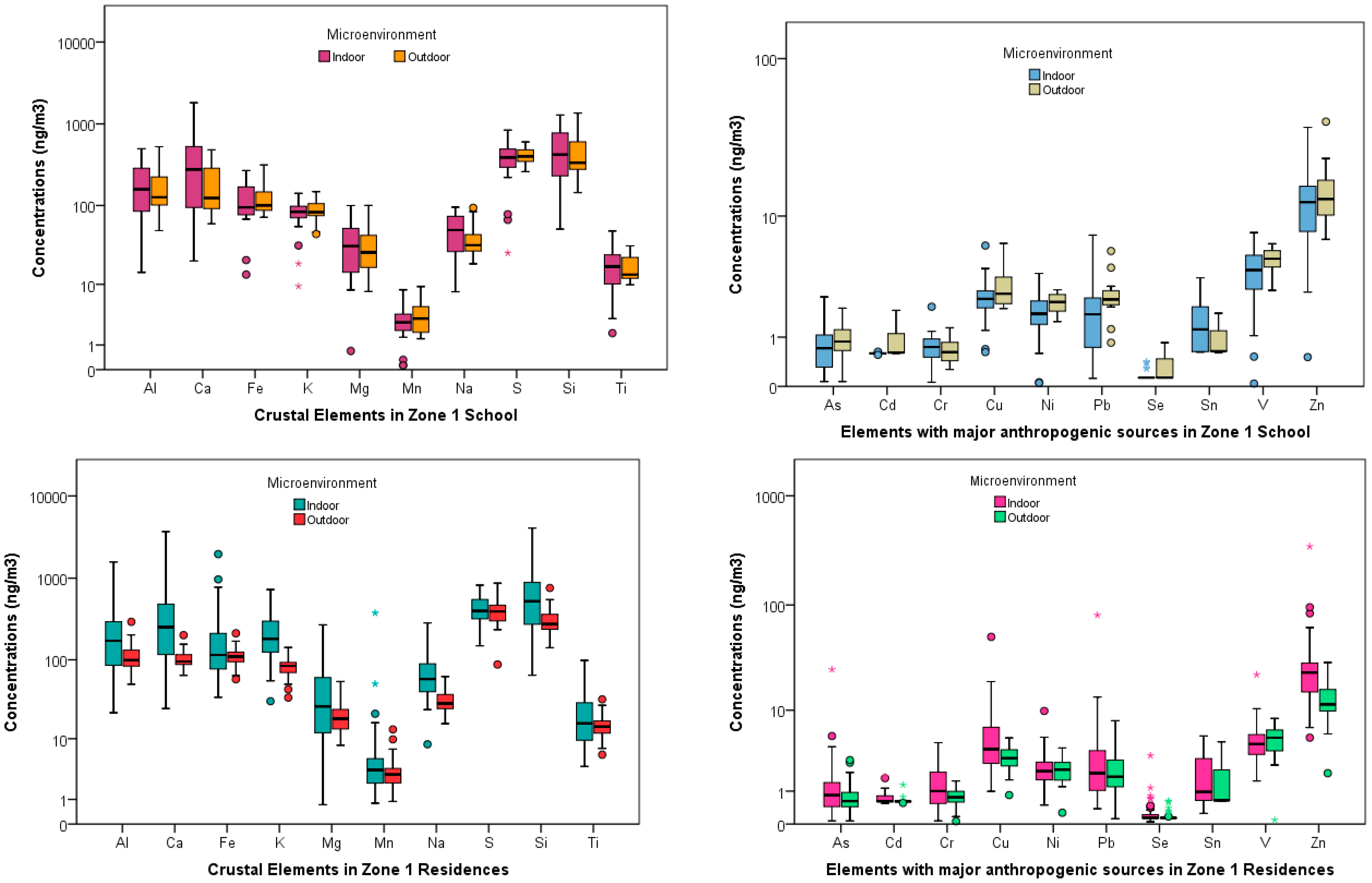
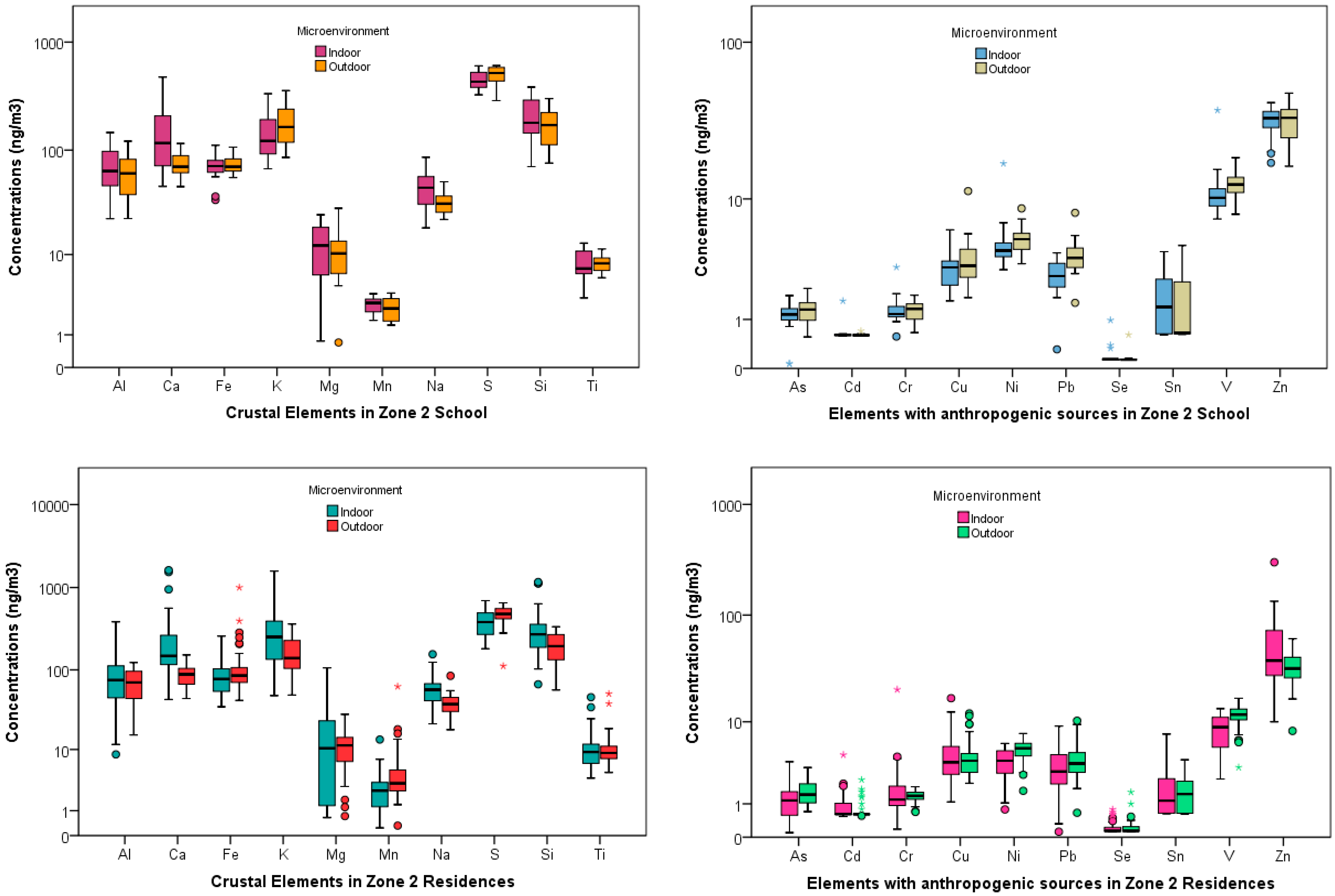
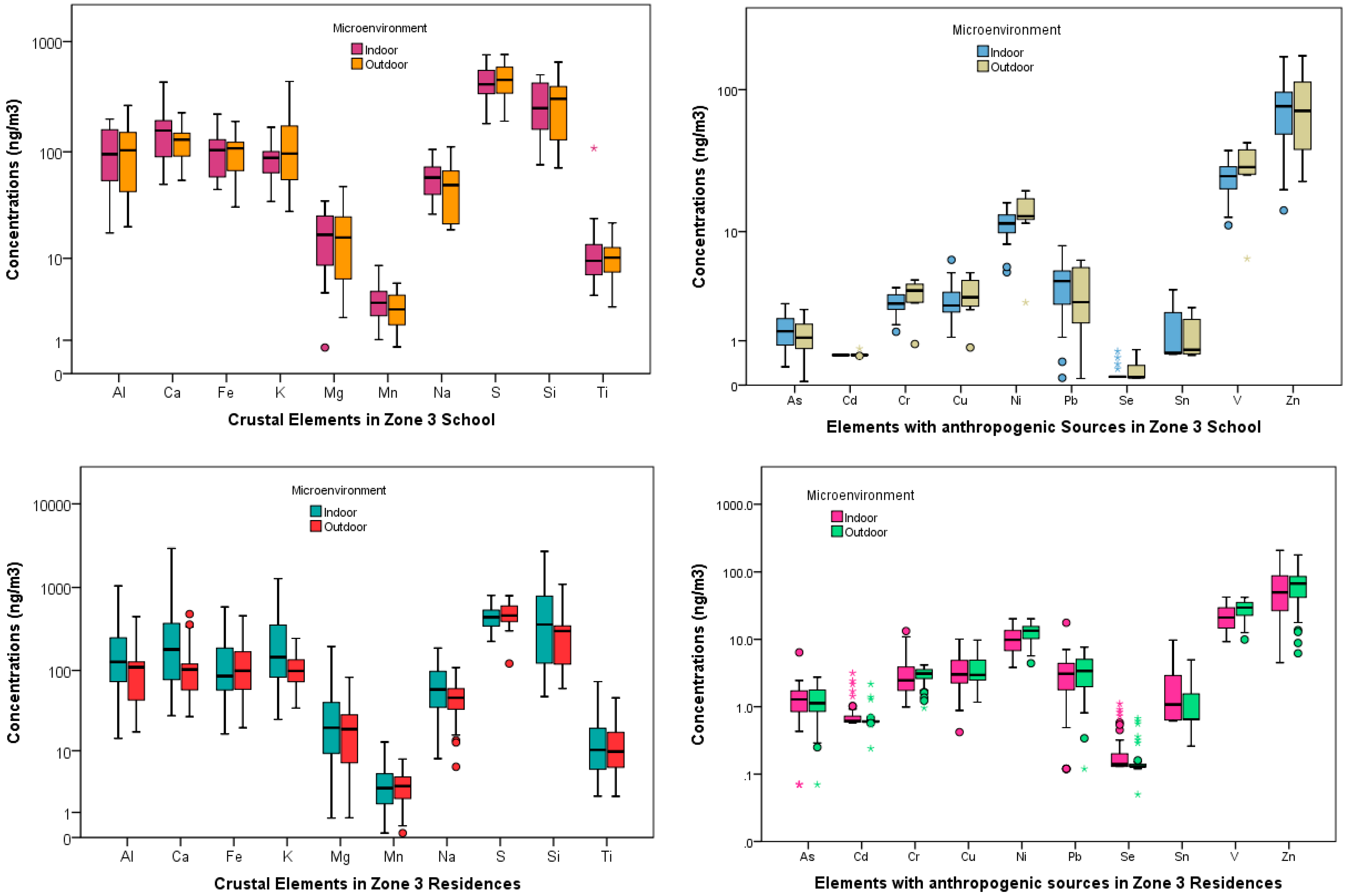
School and Residences Elemental Concentrations
4. Discussion
4.1. Indoor-Outdoor Relationships at the Three Schools
4.2. Inter-Element Correlation Relationships
4.3. Enrichment Factor Analysis
4.4. Principal Component Analysis
5. Conclusions
Acknowledgments
Author Contributions
Conflicts of Interest
References
- Brokamp, C.; Rao, M.B.; Fan, Z.; Ryan, P.H. Does the elemental composition of indoor and outdoor PM2.5 accurately represent the elemental composition of personal PM2.5? Atmos. Environ. 2015, 101, 226–234. [Google Scholar] [CrossRef]
- Oeder, S.; Dietrich, S.; Weichenmeier, I.; Schober, W.; Pusch, G.; Jorres, R.A.; Schierl, R.; Nowak, D.; Fromme, H.; Behrendt, H.; et al. Toxicity and elemental composition of particulate matter from outdoor and indoor air of elementary schools in Munich, Germany. Indoor Air 2012, 22, 148–158. [Google Scholar] [CrossRef] [PubMed]
- Dockery, D.W. Health effects of particulate air pollution. Ann. Epidemiol. 2009, 19, 257–263. [Google Scholar] [CrossRef] [PubMed]
- Sarnat, S.E.; Raysoni, A.U.; Li, W.W.; Holguin, F.; Johnson, B.A.; Luevano, S.F.; Garcia, J.H.; Sarnat, J.A. Air pollution and acute respiratory response in a panel of asthmatic children along the US–Mexico border. Environ. Health Perspect. 2012, 120, 437–444. [Google Scholar] [CrossRef] [PubMed]
- Spira-Cohen, A.; Chen, L.C.; Kendall, M.; Lall, R.; Thurston, G.D. Personal exposures to traffic-related pollution and acute respiratory health among Bronx schoolchildren with asthma. Environ. Health Perspect. 2011, 119, 559–565. [Google Scholar] [CrossRef] [PubMed]
- Kelly, F.J.; Fussell, J.C. Air pollution and airway disease. Clin. Exp. Allergy 2011, 41, 1059–1071. [Google Scholar] [CrossRef] [PubMed]
- Adar, S.D.; Sheppard, L.; Vedal, S.L.; Polak, J.F.; Sampson, P.D.; Roux, A.V.D.; Budoff, M.; Jacobs, D.R., Jr.; Barr, R.G.; Watson, K.; et al. Fine particulate air pollution and the progression of carotid intima-media thickness: A prospective cohort study from the multi-ethnic study of atherosclerosis and air pollution. PLoS Med. 2013, 10, e1001430. [Google Scholar] [CrossRef] [PubMed]
- Medina-Ramon, M.; Goldberg, R.; Melly, S.; Mittleman, M.A.; Schwartz, J. Residential exposure to traffic-related air pollution and survival after heart failure. Environ. Health Perspect. 2008, 116, 481–485. [Google Scholar] [CrossRef] [PubMed]
- Zanobetti, A.; Franklin, M.; Koutrakis, P.; Schwartz, J. Fine particulate air pollution and its components in association with cause-specific emergency admissions. Environ. Health 2009, 8, 58. [Google Scholar] [CrossRef] [PubMed]
- Bell, M.L.; Belanger, K.; Ebisu, K.; Gent, J.F.; Lee, H.J.; Koutrakis, P.; Leaderer, B.P. Prenatal exposure to fine particulate matter and birth weight: Variations by particulate constituents and sources. Epidemiology 2010, 21, 884–891. [Google Scholar] [CrossRef] [PubMed]
- Bell, M.; Ebisu, K.; Peng, R.D.; Samet, J.M.; Dominici, F. Hospital admissions and chemical composition of fine particulate air pollution. Am. J. Respir. Crit. Care Med. 2009, 179, 1115–1120. [Google Scholar] [CrossRef] [PubMed]
- Franklin, M.; Koutrakis, P.; Schwartz, P. The role of particle composition on the association between PM2.5 and mortality. Epidemiology 2008, 19, 680–689. [Google Scholar] [CrossRef] [PubMed]
- Kawata, K.; Yokoo, H.; Shimazaki, R.; Okabe, S. Classification of heavy metal toxicity by human DNA microarray analysis. Environ. Sci. Technol. 2007, 41, 3769–3774. [Google Scholar] [CrossRef] [PubMed]
- Gregoris, E.; Argiriadis, E.; Vecchaito, M.; Zambon, S.; De Pieri, S.; Donateo, A.; Contini, D.; Piazza, R.; Barbante, C.; Gambaro, A. Gas-particle distributions, sources and health effects of polycyclic aromatic hydrocarbons (PAHs), polychlorinated biphenyls (PCBs) and polychlorinated naphthalenes (PCNs) in Venice aerosols. Sci. Total Environ. 2014, 476, 393–405. [Google Scholar] [CrossRef] [PubMed]
- Kong, S.; Lu, B.; Ji, Y.; Zhao, X.; Bai, Z.; Xu, Y.; Liu, Y.; Jiang, H. Risk assessment of heavy metals in road and soil dusts within PM2.5, PM10, and PM100 fractions in Dongying city, Shandong Province, China. J. Environ. Monit. 2012, 14, 791–803. [Google Scholar] [CrossRef] [PubMed]
- United States Environmental Protection Agency (USEPA). Framework for Metals Risk Assessment EPA 120/R-7/001 March 2007. Available online: https://www.epa.gov/sites/production/files/2013-09/documents/metals-risk-assessment-final.pdf (accessed on 12 February 2017).
- International Agency for Research on Cancer (IARC). IARC Monographs on the Evaluation of Carcinogenic Risks to Humans. 2016. Available online: http://monographs.iarc.fr/ENG/Classification/latest_classif.php (accessed on 10 January 2017).
- Tchounwou, P.B.; Yedjou, C.G.; Patlolla, A.K.; Sutton, D.J. Heavy metals toxicity and the environment. Springer Basel 2012, 101, 133–164. [Google Scholar]
- Cakmak, S.; Dales, R.; Kauri, L.M.; Mahmud, M.; Ryswyk, K.V.; Vanos, J.; Liu, L.; Kumarathasan, P.; Thomson, E.; Vincent, R.; et al. Metal composition of fine particulate air pollution and acute changes in cardiorespiratory physiology. Environ. Pollut. 2014, 189, 208–214. [Google Scholar] [CrossRef] [PubMed]
- Landolph, J. Molecular mechanism of transformation of CH3/10T1/2C18 mouse embryo cells and diploid human fibroblasts by carcinogenic metal compounds. Environ. Health Perspect. 1994, 102, 119–125. [Google Scholar] [PubMed]
- Prahalad, A.K.; Inmon, J.; Dailey, L.A.; Madden, M.C.; Ghio, A.J.; Gallagher, J.E. Air pollution particles mediated oxidative DNA base damage in a cell free system and in human airway epithelial cells in relation to particulate metal content and bioreactivity. Chem. Res. Toxicol. 2001, 14, 879–887. [Google Scholar] [CrossRef] [PubMed]
- Miller, F.J. Dosimetry of particles: Critical factors having risk assessment implications. Inhal. Toxicol. 2000, 12, 389–395. [Google Scholar] [CrossRef] [PubMed]
- Saldarriaga-Norena, H.; Hernandex-Mena, L.; Ramirez-Muniz, M.; Carbajal-Romero, P.; Cosio-Ramirez, R.; Esquivel-Hernandez, B. Characterization of trace metals of risk to human health in airborne particulate matter (PM2.5) at two sites in Guadalajara, Mexico. J. Environ. Monit. 2009, 11, 887–894. [Google Scholar] [CrossRef] [PubMed]
- Stohos, S.J.; Bagchi, D. Oxidative mechanisms in the toxicity of metal ions. Free Radic. Biol. Med. 1995, 18, 321–336. [Google Scholar] [CrossRef]
- Tchounwou, P.; Newsome, C.; Williams, J.; Glass, K. Copper-induced cytotoxicity and transcriptional activation of stress genes in human live carcinoma cells. Metal Ions Biol. Med. 2008, 10, 285–290. [Google Scholar]
- Harrison, R.M.; Smith, D.J.T.; Kibble, A.J. What is responsible for the carcinogenicity of PM2.5? Occup. Environ. Med. 2003, 61, 799–805. [Google Scholar] [CrossRef] [PubMed]
- Clairborn, C.S.; Larson, T.; Sheppard, L. Testing the metals hypothesis in Spokane, Washington. Environ. Health Perspect. 2002, 110, 547–552. [Google Scholar] [CrossRef]
- Magari, S.R.; Schwarz, J.; Williams, P.L.; Hauser, R.; Smith, T.J.; Christiani, D.C. The association of particulate air metals concentrations with heart rate variability. Environ. Health Perspect. 2002, 110, 875–880. [Google Scholar] [CrossRef] [PubMed]
- Armijos, R.X.; Weigel, M.M.; Myers, O.B.; Li, W.W.; Racines, M.; Berwick, M. Residential exposure to urban traffic is associated with increased carotid intima-media thickness in children. J. Environ. Public Health 2015, 2015, 713540. [Google Scholar] [CrossRef] [PubMed]
- Bogo, H.; Otero, P.; Castro, P.; Ozafran, M.J.; Kreiner, A.; Calvo, E.J.; Negri, R.M. Study of atmospheric particulate matter in Buenos Aires city. Atmos. Environ. 2003, 37, 1135–1147. [Google Scholar] [CrossRef]
- Jurado, J.; Southgate, D. Dealing with air pollution in Latin America: The case of Quito, Ecuador. Environ. Dev. Econ. 1999, 4, 375–388. [Google Scholar] [CrossRef]
- Hassan, R.; Scholes, R.; Ash, N. (Eds.) Mountain systems. In Ecosystems and Human Well-Being: Current State and Trends; Millennium Ecosystem Assessment; Island Press: Washington, DC, USA, 2005; Chapter 24; Volume 1, p. 948. [Google Scholar]
- United Nations Environmental Program. Environment Climate Change Outlook: ECCO Metropolitan District of Quito; Regional Office for Latin America and the Caribbean, Division of Early Warning and Assessment, United Nations Environmental Program: Panama City, Panama, 2011; p. 64. [Google Scholar]
- Secretaria de Ambiente. Informe de la Calidad del Aire de Quito. 2011. Available online: http://www.quitoambiente.gob.ec (accessed on 15 October 2016).
- Brachtl, M.V.; Durant, J.L.; Perez, C.P.; Oviedo, J.; Sempertegui, F.; Naumova, E.N.; Griffiths, J.K. Spatial and temporal variations and mobile source emissions of polycyclic aromatic hydrocarbons in Quito, Ecuador. Environ. Pollut. 2009, 157, 528–536. [Google Scholar] [CrossRef] [PubMed]
- Estrella, B.; Estrella, R.; Oviedo, J.; Narvaez, X.; Reyes, M.T.; Gutierrez, M.; Naumova, E.N. Acute respiratory diseases and carboxyhemoglobin status in school children of Quito, Ecuador. Environ. Health Perspect. 2005, 113, 607–611. [Google Scholar] [CrossRef] [PubMed]
- Raysoni, A.U.; Armijos, R.X.; Weigel, M.M.; Montoya, T.; Eschanique, P.; Racines, M.; Li, W.W. Assessment of indoor and outdoor PM species at schools and residences in a high-altitude Ecuadorian urban center. Environ. Pollut. 2016, 214, 668–679. [Google Scholar] [CrossRef] [PubMed]
- Ecogestion. Desarrollo de un Instrumento para la Gestion de la Calidad del Aire en Quito: Sintesis de Proyecto y Lecciones Aprendidas. 2005. Available online: www.iadb.org/sds/doc/LeccionesAprendidasQuito.pdf (accessed on 15 October 2016).
- Corporacion para el Mejoramiento del Aire de Quito (CORPAIRE). Inventario de Emisiones Atmosferico de Quito. 2007. Available online: http://190.152.144.74/paginas/articulos.html (accessed on 20 October 2016).
- Raysoni, A.U.; Sarnat, J.A.; Sarnat, S.E.; Garcia, J.H.; Holguin, F.; Luevano, S.F.; Li, W.W. Binational school-based monitoring of traffic-related air pollutants in El Paso, Texas (USA) and Ciudad Juarez, Chihuahua (Mexico). Environ. Pollut. 2011, 159, 2476–2486. [Google Scholar] [CrossRef] [PubMed]
- Clague Romero, J.W. Experimental and Theoretical Investigation of the Mobilization, Immobilization and Sequestration of Subsurface Metals through Manipulation of Carbonate Equilibria; Paper AAI3023412; University of Texas at El Paso: El Paso, TX, USA, 2001; Available online: http://digitalcommons.utep.edu/dissertations/AAI3023412 (accessed on 9 September 2016).
- Wang, X.; Bi, X.; Sheng, G.; Fu, J. Chemical composition and sources of PM10 and PM2.5 aerosols in Guangzhou, China. Environ. Monit. Assess. 2006, 119, 425–439. [Google Scholar] [CrossRef] [PubMed]
- Hwang, Y.H.; Lin, Y.S.; Lin, C.Y.; Wang, I.J. Incense burning at home and the blood lead level of preschoolers in Taiwan. Environ. Sci. Pollut. Res. 2014, 21, 13480–13487. [Google Scholar] [CrossRef] [PubMed]
- Wasson, S.J.; Guo, Z.; McBrian, J.A.; Beach, L.O. Lead in candle emissions. Sci. Total Environ. 2002, 296, 159–174. [Google Scholar] [CrossRef]
- Chow, J.C. Measurement methods to determine compliance with ambient air quality standards for suspended particles. J. Air Waste Manag. Assoc. 1995, 45, 320–382. [Google Scholar] [CrossRef] [PubMed]
- Mazzei, F.; D’Alessandro, A.; Lucarelli, F.; Nava, S.; Prati, P.; Valli, G.; Vecchi, R. Characterization of particulate matter sources in an urban environment. Sci. Total Environ. 2008, 401, 81–89. [Google Scholar] [CrossRef] [PubMed]
- Schwander, S.; Okello, C.D.; Freers, J.; Chow, J.C.; Watson, J.G.; Corry, M.; Meng, Q. Ambient particulate matter air pollution in Mpererwe District, Kampala, Uganda: A pilot study. J. Environ. Public Health 2014, 2014, 763934. [Google Scholar] [CrossRef] [PubMed]
- Cesari, D.; Genga, A.; Ielpo, P.; Siciliano, M.; Mascolo, G.; Grasso, F.M.; Contini, D. Source apportionment of PM2.5 in the harbor-industrial area of Brindisi (Italy): Identification and estimation of the contribution of in-port ship emissions. Sci. Total Environ. 2014, 497–498, 392–400. [Google Scholar] [CrossRef] [PubMed]
- Braga, C.F.; Teixeira, E.C.; Meira, L.; Wiegand, F.; Yoneama, M.L.; Dias, J.F. Elemental composition of PM10 and PM2.5 in urban environment in South Brazil. Atmos. Environ. 2005, 39, 1801–1815. [Google Scholar] [CrossRef]
- Manno, E.; Varrica, D.; Dongarra, G. Metal distribution in road dust samples collected in an urban area close to a petrochemical plant at Gela, Sicily. Atmos. Environ. 2006, 40, 5929–5941. [Google Scholar] [CrossRef]
- Xu, L.; Yu, Y.; Yu, J.; Chen, J.; Niu, Z.; Yin, L.; Zhang, F.; Liao, X.; Chen, Y. Spatial distribution and sources identification of elements in PM2.5 among the coastal city group in the Western Taiwan Strait region, China. Sci. Total Environ. 2013, 442, 77–85. [Google Scholar] [CrossRef] [PubMed]
- Likuku, A.S.; Mmolawa, K.B.; Gaboutloeloe, G.K. Assessment of heavy metal enrichment and degree of contamination around the Copper-Nickel mine in the Selebi Phikwe Region, Eastern Botswana. Environ. Ecol. Res. 2013, 1, 32–40. [Google Scholar]
- Kim, M.K.; Jo, W.K. Elemental composition and source characterization of airborne PM10 at residences with relative proximities to metal-industrial complex. Int. Arch. Occup. Environ. Health 2006, 80, 40–50. [Google Scholar] [CrossRef] [PubMed]
- Ergenekon, P.; Ulutas, K. Heavy metal content of total suspended air particles in the heavily industrialized town of Gebze, Turkey. Bull. Environ. Contam. Toxicol. 2014, 92, 90–95. [Google Scholar] [CrossRef] [PubMed]
- Celo, V.; Dabek-Zlotorzynska, E. Concentration and source origin of trace metals in PM2.5 collected at selected Canadian sites within the Canadian national air pollution surveillance program. In Urban Airborne Particulate Matter: Origin, Chemistry, Fate and Health Impacts, 1st ed.; Zereini, F., Wiseman, C.L.S., Eds.; Springer: Berlin/Heidelberg, Germany, 2011; pp. 19–38. [Google Scholar]
- Huang, S.S.; Tu, J.; Liu, H.Y.; Hua, M.; Liao, Q.L.; Feng, J.S.; Weng, Z.H.; Huang, G.M. Multivariate analysis of trace element concentrations in atmospheric deposition in the Yangtze River Delta, East China. Atmos. Environ. 2009, 43, 5781–5790. [Google Scholar] [CrossRef]
- Taylor, S.R.; McLennan, S.M. The Continental Crust: Its Composition and Evaluation; Blackwell Scientific Publication: Oxford, UK, 1985; p. 353. [Google Scholar]
- Taner, S.; Pekey, B.; Pekey, H. Fine particulate matter in the indoor air of barbeque restaurants: Elemental compositions, sources, and health risks. Sci. Total Environ. 2013, 454–455, 79–87. [Google Scholar] [CrossRef] [PubMed]
- Cesari, D.; Contini, D.; Genga, A.; Siciliano, M.; Elefante, C.; Baglivi, F.; Daniele, L. Analysis of raw soils and their re-suspended PM10 fractions: Characterization of source profiles and enrichment factors. Appl. Geochem. 2012, 27, 1238–1246. [Google Scholar] [CrossRef]
- Ragosta, M.; Caggiano, R.; Macchiato, M.; Sabia, S.; Trippetta, S. Trace elements in daily collected aerosol: Level characterization and source identification in a four-year study. Atmos. Res. 2008, 89, 206–217. [Google Scholar] [CrossRef]
- Swietlicki, E.; Puri, S.; Hansson, H.C. Urban air pollution source apportionment using a combination of aerosol and gas monitoring techniques. Atmos. Environ. 1996, 15, 2795–2809. [Google Scholar] [CrossRef]
- Zabalza, J.; Ogulei, D.; Hopke, P.K.; Lee, J.H.; Hwang, I.; Querol, X.; Alastuey, A.S.; Santamaria, J.M. Concentration and sources of PM10 and its constituents in Alsasua, Spain. Water Air Soil Pollut. 2006, 174, 385–404. [Google Scholar] [CrossRef]
- Han, I.; Mihalic, J.N.; Ramos-Bonilla, J.P.; Rule, A.M.; Polyak, L.M.; Peng, R.D.; Geyh, A.S.; Breysse, P.N. Assessment of heterogeneity of metal composition of fine particulate matter collected from eight US counties using principal component analysis. J. Air Waste Manag. Assoc. 2012, 62, 773–782. [Google Scholar] [CrossRef] [PubMed]
- Lim, J.M.; Jeong, J.H.; Lee, J.H.; Moon, J.H.; Chung, Y.S.; Kim, K.H. The analysis of PM2.5 and associated elements and their indoor/outdoor pollution status in an urban area. Indoor Air 2011, 21, 145–155. [Google Scholar] [CrossRef] [PubMed]
- Pakkanen, T.A.; Loukkola, K.; Korhonen, C.H.; Aurela, M.; Makela, T.; Hillamo, R.E.; Aarnio, P.; Koskentalo, T.; Kousa, A.; Maenhaut, W. Sources and chemical composition of atmospheric fine and coarse particles in the Helsinki area. Atmos. Environ. 2001, 35, 5381–5391. [Google Scholar] [CrossRef]
- Kim, B.M.; Henry, R.C. Extension of self-modeling curve resolution to mixtures of more than three components: Part 3. Atmospheric aerosol data simulation studies. Chemom. Intell. Lab. Syst. 2000, 52, 145–154. [Google Scholar] [CrossRef]
- Gemenetzis, P.; Moussas, P.; Arditsoglou, A.; Samara, C. Mass concentration and elemental composition of indoor PM2.5 and PM10 in university rooms in Thessaloniki, northern Greece. Atmos. Environ. 2006, 40, 3195–3206. [Google Scholar] [CrossRef]
- Landsberger, S.; Wu, D. The impact of heavy metals from environmental tobacco smoke on indoor air quality as determined by Compton suppression neutron activation analysis. Sci. Total Environ. 1995, 173–174, 323–337. [Google Scholar] [CrossRef]
- Slezakova, K.; Pereira, M.C.; Alvim-Ferraz, M.C. Influence of tobacco smoke on the elemental composition of indoor particles of different sizes. Atmos. Environ. 2009, 43, 486–493. [Google Scholar] [CrossRef]
- Gomez, D.R.; Gine, M.F.; Bellato, A.C.S.; Smichowski, P. Antimony: A traffic-related elements in the atmosphere of Buenos Aires, Argentina. J. Environ. Monit. 2005, 7, 1162–1168. [Google Scholar] [CrossRef] [PubMed]
- Lough, G.C.; Schauer, J.J.; Park, J.S.; Shafer, M.M.; Deminter, J.T.; Weinstein, J.P. Emissions of metals associated with motor vehicle roadways. Environ. Sci. Technol. 2005, 39, 826–836. [Google Scholar] [CrossRef] [PubMed]
- Majestic, B.J.; Turner, J.A.; Marcotte, A.R. Respirable antimony and other trace-elements inside and outside an elementary school in Flagstaff, AZ, USA. Sci. Total Environ. 2012, 435–436, 253–261. [Google Scholar] [CrossRef] [PubMed]
- Furuta, N.; Iijima, A.; Kambe, A.; Sakai, K.; Sato, K. Concentrations, enrichment and predominant sources of Sb and other trace elements in size classified airborne particulate matter collected in Tokyo from 1995 to 2004. J. Environ. Monit. 2005, 7, 1155–1161. [Google Scholar] [CrossRef] [PubMed]
- Dobrowolski, R.; Dobrzynska, J.; Gawronska, B. Determination of bismuth in environmental samples by slurry sampling graphite furnace atomic absorption spectrometry using combined chemical modifiers. Environm. Monit. Assess. 2015, 187, 4125. [Google Scholar] [CrossRef] [PubMed]
- Wiseman, C.L.S.; Zereini, F. Airborne particulate matter, platinum group elements and human health: A review of recent evidence. Sci. Total Environ. 2009, 407, 2493–2500. [Google Scholar] [CrossRef] [PubMed]
- Kielhorn, J.; Melber, C.; Keller, D.; Mangelsdorf, I. Palladium—A review of exposure and effects to human health. Int. J. Hyg. Environ. Health 2002, 205, 417–432. [Google Scholar] [CrossRef] [PubMed]
- Fathi, Z.; Alt, F.; Messerschmidt, J.; Wiseman, C.; Feldmann, I.; von Bohlen, A.; Muller, J.; Liebl, K.; Puttmann, W. Concentration and particle size distribution of heavy metals in urban airborne particulate matter in Frankfurt am Main, Germany. Environ. Sci. Technol. 2005, 39, 2983–2989. [Google Scholar]
- Lin, C.W.; Chen, Y.R.; Yen, C.H.; Kao, T.C. Chemical mass balance source apportionment of ambient total suspended particulate matters near Jhuoshuei river in Central Taiwan. Environ. Forensics 2010, 11, 216–222. [Google Scholar] [CrossRef]
- Alastuey, A.; Querol, X.; Plana, F.; Viana, M.; Ruiz, C.R.; Campa, A.S.D.L.; Rosa, J.D.L.; Mantilla, E.; Santosm, S.G.D. Identification and chemical characterization of industrial particulate matter sources in southwest Spain. J. Air Waste Manag. Assoc. 2006, 56, 993–1006. [Google Scholar] [CrossRef] [PubMed]
- Belis, C.A.; Karagulian, F.; Larsen, B.R.; Hopke, P.K. Critical review and meta-analysis of ambient particulate matter source apportionment using receptor models in Europe. Atmos. Environ. 2013, 69, 94–108. [Google Scholar] [CrossRef]
- Viana, M.; Kuhlbusch, T.A.J.; Querol, X.; Alastuey, A.; Harrison, R.M.; Hopke, P.K.; Winiwarter, W.; Vallius, M.; Szidat, S.; Prevot, A.S.H.; et al. Source apportionment of particulate matter in Europe: A review of methods and results. J. Aerosol Sci. 2008, 39, 827–849. [Google Scholar] [CrossRef]
- Nriagu, J.; Davidson, C. Toxic Metals in the Atmosphere, 1st ed.; Wiley Interscience Publications: Hoboken, NJ, USA, 1986; p. 635. [Google Scholar]
- Lopez, M.L.; Ceppi, S.; Palancar, G.G.; Olcese, L.E.; Tirao, G.; Toselli, B.M. Elemental concentration and source identification of PM10 and PM2.5 by SR-XRF in Cordoba City, Argentina. Atmos. Environ. 2011, 45, 5450–5457. [Google Scholar] [CrossRef]
- Cong, Z.Y.; Kang, S.C.; Liu, X.D.; Wang, G.F. Elemental composition of aerosol in the Nam Co region, Tibetan Plateau, during summer monsoon season. Atmos. Environ. 2007, 41, 1180–1187. [Google Scholar] [CrossRef]
- Lucarelli, F.; Mando, A.; Nava, S.; Prati, P.; Zucchiatti, A. One year study of the elemental composition and source apportionment of PM10 aerosols in Florence, Italy. J. Air Waste Manag. Assoc. 2004, 54, 1372–1382. [Google Scholar] [CrossRef] [PubMed]
- Demoisson, A.; Tedeschi, G.; Piassola, J. A model for the atmospheric transport of sea-salt particles in coastal areas. Atmos. Res. 2013, 132–133, 144–153. [Google Scholar] [CrossRef]
- Martello, D.V.; Pekney, N.J.; Anderson, R.R.; Davidson, C.I.; Hopke, P.K.; Kim, E.; Christensen, W.F.; Mangelson, N.F.; Eatough, D.J. Apportionment of ambient primary and secondary fine particulate matter at the Pittsburgh National Energy Laboratory particulate matter characterization site using positive matrix factorization and a potential source contributions function analysis. J. Air Waste Manag. Assoc. 2008, 58, 357–368. [Google Scholar] [PubMed]
- Waheed, S.; Jaafar, M.Z.; Siddique, N.; Markwitz, A.; Brereton, R.G. PIXE Analysis of PM2.5 and PM2.5−10 for air quality assessment of Islamabad, Pakistan: Application of chemometrics for source identification. J. Environ. Sci. Health 2012, 47, 2016–2027. [Google Scholar] [CrossRef] [PubMed]


| Elements | DL |
|---|---|
| Na | 0.0085 |
| Mg | 0.0106 |
| Al | 0.0089 |
| Si | 0.0044 |
| S | 0.0010 |
| K | 0.0011 |
| Ca | 0.0017 |
| Sc | 0.0034 |
| Ti | 0.0010 |
| V | 0.0006 |
| Cr | 0.0009 |
| Mn | 0.0020 |
| Fe | 0.0020 |
| Co | 0.0005 |
| Ni | 0.0008 |
| Cu | 0.0013 |
| Zn | 0.0014 |
| As | 0.0010 |
| Se | 0.0020 |
| Rb | 0.0007 |
| Sr | 0.0013 |
| Y | 0.0011 |
| Mo | 0.0028 |
| Rh | 0.0033 |
| Pd | 0.0065 |
| Ag | 0.0069 |
| Cd | 0.0088 |
| Sn | 0.0094 |
| Sb | 0.0086 |
| Te | 0.0102 |
| Cs | 0.0117 |
| Ba | 0.0127 |
| W | 0.0222 |
| Pt | 0.0056 |
| Au | 0.0046 |
| Pb | 0.0018 |
| Bi | 0.0043 |
| La | 0.0189 |
| Th | 0.0053 |
| Zones | Z1 | Z2 | Z3 | |||
|---|---|---|---|---|---|---|
| Schools | Indoor (n = 23) | Outdoor (n = 10) | Indoor (n = 16) | Outdoor (n = 11) | Indoor (n = 19) | Outdoor (n = 10) |
| Elements | Mean ± SD | Mean ± SD | Mean ± SD | Mean ± SD | Mean ± SD | Mean ± SD |
| PM2.5 | 10.70 ± 4.94 | 10.87 ± 3.23 | 14.66 ± 15.64 | 13.19 ± 3.47 | 10.83 ± 8.85 | 12.98 ± 8.71 |
| Al | 192.49 ± 135.38 | 198.51 ± 165.78 | 71.75 ± 36.38 | 63.66 ± 33.68 | 102.38 ± 59.31 | 106.01 ± 74.12 |
| Ca | 406.64 ± 424.17 | 193.97 ± 146.32 | 163.27 ± 134.24 | 75.27 ± 23.10 | 164.12 ± 108.28 | 124.99 ± 49.40 |
| Fe | 123.65 ± 68.58 | 139.14 ± 87.90 | 70.12 ± 19.19 | 76.10 ± 17.23 | 99.73 ± 47.56 | 100.53 ± 43.80 |
| K | 80.85 ± 31.05 | 88.58 ± 31.25 | 152.00 ± 76.25 | 186.54 ± 90.51 | 90.79 ± 39.23 | 129.81 ± 118.55 |
| Mg | 37.00 ± 28.35 | 36.67 ± 30.76 | 12.49 ± 7.56 | 11.16 ± 7.68 | 17.87 ± 11.17 | 18.25 ± 15.21 |
| Mn | 3.15 ± 2.07 | 3.86 ± 2.46 | 2.81 ± 0.66 | 2.51 ± 0.91 | 3.55 ± 1.72 | 2.98 ± 1.51 |
| Na | 49.42 ± 28.40 | 41.48 ± 25.31 | 45.74 ± 18.08 | 32.93 ± 9.45 | 60.47 ± 23.14 | 53.02 ± 30.18 |
| S | 400.55 ± 208.62 | 412.45 ± 99.56 | 447.63 ± 87.53 | 503.43 ± 101.78 | 437.22 ± 144.75 | 463.19 ± 162.04 |
| Si | 524.08 ± 360.25 | 535.58 ± 432.47 | 204.19 ± 93.08 | 173.23 ± 78.16 | 276.60 ± 141.20 | 290.83 ± 179.77 |
| Ti | 18.69 ± 11.60 | 17.74 ± 7.99 | 8.18 ± 2.86 | 8.24 ± 1.82 | 15.57 ± 23.01 | 10.67 ± 5.13 |
| As | 0.83 ± 0.71 | 0.91 ± 0.55 | 1.09 ± 0.46 | 1.29 ± 0.48 | 1.36 ± 0.59 | 1.17 ± 0.64 |
| Cd | 0.59 ± 0.02 | 0.91 ± 0.50 | 0.66 ± 0.25 | 0.61 ± 0.03 | 0.60 ± 0.01 | 0.61 ± 0.06 |
| Cr | 0.75 ± 0.42 | 0.66 ± 0.31 | 1.32 ± 0.57 | 1.25 ± 0.34 | 2.58 ± 0.63 | 3.15 ± 0.96 |
| Cu | 2.49 ± 1.13 | 3.25 ± 1.55 | 3.27 ± 1.26 | 4.10 ± 2.65 | 2.84 ± 1.22 | 3.07 ± 1.19 |
| Ni | 1.83 ± 0.91 | 2.22 ± 0.51 | 5.15 ± 3.32 | 5.39 ± 1.51 | 11.27 ± 3.15 | 13.78 ± 4.96 |
| Pb | 2.12 ± 1.89 | 2.67 ± 1.36 | 2.75 ± 1.01 | 4.05 ± 1.69 | 3.82 ± 2.09 | 3.03 ± 2.12 |
| Se | 0.18 ± 0.10 | 0.31 ± 0.24 | 0.22 ± 0.22 | 0.18 ± 0.14 | 0.21 ± 0.16 | 0.25 ± 0.20 |
| Sn | 1.52 ± 1.05 | 0.93 ± 0.46 | 1.55 ± 1.08 | 1.70 ± 1.51 | 1.28 ± 0.94 | 1.18 ± 0.69 |
| V | 4.04 ± 1.98 | 4.95 ± 1.20 | 11.95 ± 7.13 | 12.73 ± 3.07 | 24.81 ± 6.89 | 30.14 ± 10.50 |
| Zn | 13.19 ± 7.92 | 15.60 ± 9.77 | 31.99 ± 7.35 | 32.48 ± 9.96 | 77.17 ± 42.76 | 77.21 ± 48.50 |
| Ag | 0.51 ± 0.22 | 0.49 ± 0.06 | 0.47 ± 0.01 | 0.47 ± 0.02 | 0.47 ± 0.01 | 0.48 ± 0.04 |
| Au | 0.50 ± 0.31 | 0.77 ± 0.65 | 0.50 ± 0.35 | 0.72 ± 0.66 | 0.84 ± 0.75 | 0.45 ± 0.41 |
| Ba | 7.23 ± 5.01 | 11.17 ± 6.78 | 4.91 ± 3.79 | 8.57 ± 5.03 | 7.51 ± 5.45 | 7.52 ± 4.82 |
| Bi | 0.50 ± 0.35 | 0.51 ± 0.45 | 0.47 ± 0.32 | 0.73 ± 0.63 | 0.40 ± 0.31 | 0.54 ± 0.39 |
| Co | 0.14 ± 0.21 | 0.30 ± 0.76 | 0.12 ± 0.22 | 0.04 ± 0.02 | 0.16 ± 0.36 | 0.05 ± 0.07 |
| Cs | 1.08 ± 1.12 | 1.35 ± 0.90 | 1.33 ± 1.08 | 0.97 ± 0.53 | 1.34 ± 1.08 | 0.91 ± 0.26 |
| La | 3.07 ± 2.61 | 2.70 ± 1.81 | 4.70 ± 3.51 | 2.75 ± 2.04 | 3.36 ± 2.35 | 3.70 ± 2.43 |
| Mo | 0.19 ± 0.00 | 0.20 ± 0.03 | 0.19 ± 0.01 | 0.20 ± 0.01 | 0.19 ± 0.00 | 0.22 ± 0.08 |
| Pd | 0.53 ± 0.46 | 0.52 ± 0.18 | 0.50 ± 0.21 | 0.65 ± 0.67 | 0.54 ± 0.42 | 0.54 ± 0.26 |
| Pt | 1.54 ± 1.08 | 1.52 ± 1.44 | 3.02 ± 1.25 | 3.10 ± 1.56 | 6.32 ± 3.50 | 6.58 ± 4.28 |
| Rb | 0.16 ± 0.22 | 0.13 ± 0.13 | 0.23 ± 0.24 | 0.21 ± 0.15 | 0.16 ± 0.19 | 0.16 ± 0.19 |
| Rh | 0.36 ± 0.28 | 0.26 ± 0.10 | 0.43 ± 0.60 | 0.49 ± 0.50 | 0.34 ± 0.34 | 0.36 ± 0.30 |
| Sb | 1.39 ± 1.04 | 0.98 ± 0.58 | 1.46 ± 1.30 | 1.24 ± 1.01 | 0.76 ± 0.46 | 0.75 ± 0.49 |
| Sc | 0.35 ± 0.29 | 0.35 ± 0.35 | 0.34 ± 0.22 | 0.24 ± 0.01 | 0.27 ± 0.14 | 0.28 ± 0.13 |
| Sr | 1.64 ± 1.08 | 1.39 ± 0.87 | 0.85 ± 0.58 | 0.74 ± 0.37 | 0.98 ± 0.56 | 0.94 ± 0.68 |
| Te | 0.99 ± 0.77 | 1.71 ± 1.25 | 1.00 ± 1.20 | 1.07 ± 1.19 | 1.50 ± 1.49 | 1.26 ± 0.83 |
| Th | 0.41 ± 0.18 | 0.51 ± 0.43 | 0.67 ± 0.57 | 0.42 ± 0.20 | 0.52 ± 0.47 | 0.48 ± 0.35 |
| U | 0.49 ± 0.49 | 0.37 ± 0.28 | 0.54 ± 0.63 | 0.47 ± 0.28 | 0.62 ± 0.70 | 0.44 ± 0.33 |
| W | 2.53 ± 1.87 | 1.57 ± 0.21 | 1.51 ± 0.04 | 2.33 ± 2.61 | 3.51 ± 3.34 | 4.62 ± 3.26 |
| Y | 0.24 ± 0.22 | 0.19 ± 0.18 | 0.25 ± 0.19 | 0.22 ± 0.16 | 0.16 ± 0.19 | 0.29 ± 0.24 |
| Zones | Z1 | Z2 | Z3 | |||
|---|---|---|---|---|---|---|
| Residences | Indoor (n = 44) | Outdoor (n = 42) | Indoor (n = 44) | Outdoor (n = 43) | Indoor (n = 40) | Outdoor (n = 41) |
| Element | Mean ± SD | Mean ± SD | Mean ± SD | Mean ± SD | Mean ± SD | Mean ± SD |
| PM2.5 | 28.95 ± 30.49 | 12.48 ± 4.55 | 20.76 ± 10.37 | 12.91 ± 3.25 | 19.32 ± 14.63 | 13.45 ± 7.22 |
| Al | 251.88 ± 283.54 | 111.36 ± 45.29 | 101.39 ± 94.42 | 70.87 ± 30.48 | 189.01 ± 193.37 | 117.74 ± 91.90 |
| Ca | 445.43 ± 662.39 | 103.91 ± 28.13 | 259.35 ± 331.08 | 87.68 ± 26.18 | 323.72 ± 508.70 | 117.83 ± 92.16 |
| Fe | 220.33 ± 328.96 | 113.16 ± 28.70 | 91.06 ± 54.35 | 128.11 ± 152.16 | 130.14 ± 116.31 | 125.30 ± 91.11 |
| K | 240.16 ± 167.16 | 82.83 ± 23.56 | 339.49 ± 323.49 | 169.21 ± 84.27 | 250.49 ± 255.29 | 106.03 ± 49.22 |
| Mg | 46.87 ± 56.22 | 20.15 ± 9.58 | 17.67 ± 23.09 | 11.30 ± 6.60 | 31.21 ± 35.48 | 21.94 ± 18.57 |
| Mn | 13.71 ± 56.28 | 3.44 ± 2.25 | 2.78 ± 2.39 | 5.92 ± 9.66 | 3.57 ± 2.96 | 3.33 ± 2.00 |
| Na | 75.82 ± 57.34 | 31.96 ± 10.19 | 59.65 ± 27.24 | 38.27 ± 11.69 | 68.38 ± 45.93 | 48.31 ± 25.10 |
| S | 444.02 ± 167.26 | 421.20 ± 164.16 | 394.62 ± 134.31 | 476.52 ± 104.85 | 461.82 ± 144.53 | 493.21 ± 157.47 |
| Si | 726.24 ± 759.68 | 308.28 ± 115.27 | 346.62 ± 275.05 | 198.13 ± 77.35 | 508.89 ± 530.59 | 312.47 ± 233.59 |
| Ti | 22.40 ± 19.47 | 15.41 ± 5.37 | 11.26 ± 7.91 | 11.14 ± 8.14 | 16.23 ± 17.31 | 12.82 ± 9.33 |
| As | 1.67 ± 3.74 | 0.79 ± 0.60 | 1.27 ± 0.92 | 1.56 ± 0.63 | 1.39 ± 1.05 | 1.25 ± 0.67 |
| Cd | 0.74 ± 0.26 | 0.63 ± 0.11 | 0.91 ± 0.68 | 0.74 ± 0.36 | 0.84 ± 0.57 | 0.67 ± 0.30 |
| Cr | 1.26 ± 0.97 | 0.78 ± 0.32 | 1.88 ± 3.02 | 1.36 ± 0.26 | 3.38 ± 2.70 | 2.92 ± 0.81 |
| Cu | 6.50 ± 8.27 | 3.07 ± 0.88 | 4.92 ± 3.51 | 4.43 ± 2.43 | 3.72 ± 2.27 | 3.72 ± 2.05 |
| Ni | 2.34 ± 1.53 | 2.19 ± 0.75 | 3.77 ± 1.45 | 5.20 ± 1.36 | 10.57 ± 4.60 | 12.97 ± 3.88 |
| Pb | 4.45 ± 12.02 | 2.19 ± 1.56 | 3.47 ± 2.32 | 4.02 ± 1.82 | 3.29 ± 2.93 | 3.48 ± 1.99 |
| Se | 0.32 ± 0.51 | 0.19 ± 0.13 | 0.22 ± 0.16 | 0.24 ± 0.26 | 0.25 ± 0.25 | 0.18 ± 0.13 |
| Sn | 1.77 ± 1.39 | 1.37 ± 1.09 | 1.68 ± 1.42 | 1.60 ± 0.99 | 1.95 ± 1.81 | 1.22 ± 1.13 |
| V | 4.88 ± 3.25 | 5.03 ± 1.73 | 8.29 ± 3.18 | 11.72 ± 2.87 | 22.72 ± 9.69 | 28.43 ± 8.23 |
| Zn | 33.99 ± 51.74 | 12.46 ± 4.84 | 53.59 ± 48.12 | 33.60 ± 10.43 | 59.57 ± 44.25 | 69.11 ± 41.12 |
| Ag | 0.59 ± 0.33 | 0.48 ± 0.02 | 0.55 ± 0.14 | 0.48 ± 0.05 | 0.51 ± 0.10 | 0.47 ± 0.05 |
| Au | 0.77 ± 0.65 | 0.52 ± 0.37 | 0.98 ± 0.99 | 0.66 ± 0.57 | 0.64 ± 0.57 | 0.61 ± 0.46 |
| Ba | 10.34 ± 9.26 | 11.22 ± 6.06 | 6.43 ± 4.71 | 6.93 ± 4.55 | 8.55 ± 6.54 | 14.52 ± 14.59 |
| Bi | 0.74 ± 0.61 | 0.68 ± 0.57 | 0.75 ± 0.59 | 0.56 ± 0.40 | 0.59 ± 0.50 | 0.40 ± 0.34 |
| Co | 0.33 ± 0.62 | 0.17 ± 0.35 | 0.36 ± 1.52 | 0.17 ± 0.29 | 0.19 ± 0.35 | 0.16 ± 0.36 |
| Cs | 1.48 ± 1.35 | 1.24 ± 1.40 | 1.47 ± 1.39 | 1.81 ± 1.66 | 1.80 ± 1.64 | 1.43 ± 1.49 |
| La | 4.63 ± 3.67 | 2.71 ± 2.39 | 4.55 ± 4.77 | 3.88 ± 4.02 | 4.89 ± 4.43 | 2.54 ± 2.15 |
| Mo | 0.24 ± 0.14 | 0.20 ± 0.01 | 0.25 ± 0.14 | 0.20 ± 0.02 | 0.21 ± 0.04 | 0.21 ± 0.09 |
| Pd | 0.59 ± 0.34 | 0.50 ± 0.30 | 0.56 ± 0.20 | 0.58 ± 0.28 | 0.57 ± 0.28 | 0.46 ± 0.13 |
| Pt | 3.41 ± 5.26 | 1.33 ± 1.00 | 4.49 ± 4.32 | 3.25 ± 1.58 | 5.65 ± 4.11 | 5.95 ± 3.61 |
| Rb | 0.18 ± 0.27 | 0.16 ± 0.16 | 0.23 ± 0.24 | 0.33 ± 0.30 | 0.29 ± 0.30 | 0.18 ± 0.18 |
| Rh | 0.35 ± 0.33 | 0.27 ± 0.19 | 0.43 ± 0.46 | 0.33 ± 0.33 | 0.34 ± 0.30 | 0.40 ± 0.50 |
| Sb | 1.24 ± 1.30 | 1.29 ± 1.18 | 1.70 ± 2.55 | 1.57 ± 1.58 | 1.51 ± 1.52 | 1.40 ± 1.52 |
| Sc | 0.40 ± 0.41 | 0.25 ± 0.06 | 0.32 ± 0.22 | 0.32 ± 0.28 | 0.36 ± 0.35 | 0.28 ± 0.19 |
| Sr | 2.19 ± 2.54 | 0.99 ± 0.44 | 1.04 ± 1.06 | 0.68 ± 0.36 | 1.60 ± 1.78 | 1.26 ± 1.08 |
| Te | 1.70 ± 1.59 | 1.13 ± 0.85 | 1.50 ± 1.44 | 1.42 ± 1.45 | 1.14 ± 0.71 | 1.16 ± 0.80 |
| Th | 0.52 ± 0.43 | 0.42 ± 0.23 | 0.64 ± 0.60 | 0.48 ± 0.31 | 0.57 ± 0.43 | 0.47 ± 0.29 |
| U | 0.54 ± 0.38 | 0.53 ± 0.41 | 0.66 ± 0.59 | 0.49 ± 0.38 | 0.53 ± 0.47 | 0.43 ± 0.39 |
| W | 5.31 ± 17.78 | 2.09 ± 2.00 | 2.73 ± 2.18 | 2.33 ± 2.14 | 4.28 ± 4.17 | 3.38 ± 3.32 |
| Y | 0.27 ± 0.25 | 0.21 ± 0.20 | 0.26 ± 0.22 | 0.23 ± 0.17 | 0.20 ± 0.16 | 0.20 ± 0.20 |
| Zone 1 (n = 19) | Zone 2 (n = 14) | Zone 3 (n = 17) | ||||||||||||||||
|---|---|---|---|---|---|---|---|---|---|---|---|---|---|---|---|---|---|---|
| Elements | Mean | Median | Stdev | Min | Max | p-Value | Mean | Median | Stdev | Min | Max | p-Value | Mean | Median | Stdev | Min | Max | p-Value |
| PM2.5 | 1.00 | 0.93 | 0.59 | 0.02 | 2.54 | 0.453 | 1.23 | 0.91 | 1.15 | 0.34 | 5.03 | 0.541 | 1.06 | 0.95 | 0.61 | 0.38 | 2.86 | 0.719 |
| Al | 1.23 | 0.94 | 1.03 | 0.09 | 4.13 | 0.651 | 1.43 | 1.17 | 1.49 | 0.50 | 6.44 | 0.518 | 1.11 | 1.03 | 0.57 | 0.30 | 2.42 | 0.501 |
| Ca | 2.61 | 1.45 | 2.86 | 0.15 | 9.54 | 0.058 | 2.31 | 1.34 | 2.53 | 0.69 | 10.45 | 0.034 | 1.33 | 1.15 | 0.85 | 0.37 | 3.26 | 0.219 |
| Fe | 1.04 | 0.86 | 0.67 | 0.11 | 2.71 | 0.357 | 0.92 | 0.93 | 0.26 | 0.53 | 1.50 | 0.206 | 1.07 | 0.97 | 0.53 | 0.36 | 2.46 | 0.793 |
| K | 0.95 | 0.96 | 0.42 | 0.08 | 1.99 | 0.176 | 0.89 | 0.97 | 0.21 | 0.41 | 1.14 | 0.043 | 1.10 | 0.96 | 0.77 | 0.21 | 3.32 | 0.267 |
| Mg | 1.25 | 0.96 | 0.95 | 0.02 | 3.45 | 0.843 | 3.26 | 1.06 | 7.65 | 0.29 | 29.63 | 0.456 | 1.40 | 1.14 | 1.09 | 0.19 | 3.98 | 0.539 |
| Mn | 1.04 | 0.95 | 0.71 | 0.02 | 2.63 | 0.319 | 1.10 | 1.10 | 0.22 | 0.78 | 1.63 | 0.292 | 1.38 | 0.98 | 1.18 | 0.49 | 5.58 | 0.424 |
| Na | 1.43 | 1.01 | 1.20 | 0.17 | 5.12 | 0.359 | 1.39 | 1.27 | 0.49 | 0.58 | 2.40 | 0.009 | 1.27 | 1.03 | 0.60 | 0.64 | 2.70 | 0.363 |
| S | 0.88 | 1.00 | 0.34 | 0.05 | 1.31 | 0.112 | 0.95 | 0.96 | 0.19 | 0.63 | 1.41 | 0.168 | 1.12 | 0.97 | 0.63 | 0.59 | 3.11 | 0.878 |
| Si | 1.23 | 0.91 | 1.01 | 0.12 | 3.92 | 0.697 | 1.37 | 1.21 | 1.12 | 0.52 | 5.08 | 0.354 | 1.06 | 1.03 | 0.45 | 0.32 | 2.02 | 0.413 |
| Ti | 1.09 | 1.01 | 0.59 | 0.11 | 2.35 | 0.765 | 1.05 | 0.99 | 0.47 | 0.43 | 2.08 | 0.977 | 1.36 | 1.09 | 1.07 | 0.30 | 4.89 | 0.307 |
| As | 1.20 | 0.98 | 1.15 | 0.05 | 5.03 | 0.853 | 0.92 | 0.90 | 0.57 | 0.08 | 2.09 | 0.212 | 4.23 | 0.99 | 9.23 | 0.39 | 28.98 | 0.535 |
| Cd | 0.78 | 0.97 | 0.28 | 0.31 | 1.01 | 0.005 | 1.12 | 1.01 | 0.45 | 0.93 | 2.67 | 0.343 | 0.98 | 0.99 | 0.08 | 0.77 | 1.07 | 0.262 |
| Cr | 1.29 | 1.08 | 0.80 | 0.07 | 3.35 | 0.419 | 1.09 | 0.95 | 0.66 | 0.38 | 3.12 | 0.911 | 0.98 | 0.89 | 0.41 | 0.58 | 2.22 | 0.052 |
| Cu | 0.82 | 0.90 | 0.30 | 0.16 | 1.25 | 0.013 | 0.97 | 1.00 | 0.29 | 0.49 | 1.54 | 0.342 | 1.14 | 0.94 | 0.77 | 0.46 | 3.23 | 0.715 |
| Ni | 0.85 | 0.93 | 0.39 | 0.02 | 1.37 | 0.088 | 1.05 | 0.84 | 0.89 | 0.57 | 4.10 | 0.922 | 1.05 | 0.92 | 0.61 | 0.51 | 3.04 | 0.074 |
| Pb | 0.91 | 0.83 | 0.73 | 0.03 | 2.77 | 0.246 | 0.80 | 0.69 | 0.43 | 0.10 | 1.77 | 0.023 | 8.65 | 1.02 | 15.84 | 0.07 | 52.03 | 0.370 |
| Se | 1.00 | 0.98 | 0.98 | 0.15 | 3.15 | 0.038 | 1.65 | 1.01 | 1.79 | 0.22 | 7.42 | 0.437 | 1.13 | 1.00 | 0.97 | 0.18 | 4.11 | 0.417 |
| Sn | 2.04 | 1.02 | 1.82 | 0.35 | 5.67 | 0.054 | 1.80 | 0.99 | 1.86 | 0.39 | 6.82 | 0.561 | 1.80 | 1.00 | 1.67 | 0.28 | 5.24 | 0.316 |
| V | 0.83 | 0.92 | 0.35 | 0.01 | 1.22 | 0.040 | 1.03 | 0.86 | 0.86 | 0.51 | 3.98 | 0.846 | 1.05 | 0.93 | 0.63 | 0.49 | 3.11 | 0.087 |
| Zn | 1.06 | 1.03 | 0.64 | 0.04 | 2.88 | 0.517 | 0.99 | 0.95 | 0.35 | 0.55 | 1.80 | 0.282 | 1.08 | 0.92 | 0.72 | 0.59 | 3.49 | 0.387 |
| Ag | 1.04 | 0.99 | 0.29 | 0.68 | 2.26 | 0.530 | 1.00 | 1.00 | 0.03 | 0.93 | 1.07 | 0.676 | 0.98 | 0.99 | 0.08 | 0.77 | 1.07 | 0.262 |
| Au | 1.08 | 0.97 | 0.98 | 0.13 | 3.82 | 0.107 | 1.18 | 0.99 | 1.04 | 0.15 | 3.63 | 0.373 | 2.41 | 1.02 | 2.34 | 0.19 | 7.91 | 0.165 |
| Ba | 0.89 | 0.74 | 0.99 | 0.07 | 4.76 | 0.015 | 0.78 | 0.79 | 0.54 | 0.07 | 2.07 | 0.059 | 2.14 | 1.00 | 2.41 | 0.19 | 7.94 | 0.988 |
| Bi | 1.17 | 0.99 | 0.84 | 0.17 | 3.45 | 0.416 | 1.11 | 0.99 | 0.86 | 0.14 | 2.86 | 0.240 | 1.19 | 0.99 | 1.00 | 0.26 | 3.84 | 0.797 |
| Co | 1.93 | 1.00 | 2.86 | 0.01 | 10.18 | 0.291 | 2.94 | 1.01 | 4.51 | 0.28 | 16.50 | 0.141 | 5.12 | 0.99 | 12.07 | 0.77 | 44.71 | 0.179 |
| Cs | 1.17 | 0.98 | 1.59 | 0.26 | 7.71 | 0.444 | 1.71 | 1.01 | 1.49 | 0.30 | 5.79 | 0.193 | 1.30 | 0.99 | 1.09 | 0.49 | 5.17 | 0.380 |
| La | 1.59 | 0.99 | 1.59 | 0.19 | 4.99 | 0.583 | 2.41 | 1.04 | 2.31 | 0.23 | 7.38 | 0.145 | 1.34 | 0.99 | 1.22 | 0.16 | 4.64 | 0.490 |
| Mo | 0.96 | 0.99 | 0.10 | 0.68 | 1.10 | 0.116 | 1.00 | 1.00 | 0.03 | 0.93 | 1.07 | 0.676 | 0.91 | 0.99 | 0.19 | 0.44 | 1.07 | 0.102 |
| Pd | 1.07 | 0.99 | 0.72 | 0.43 | 4.10 | 0.807 | 1.13 | 1.00 | 0.49 | 0.93 | 2.84 | 0.354 | 1.14 | 0.99 | 1.03 | 0.35 | 5.03 | 0.978 |
| Pt | 2.08 | 1.00 | 2.13 | 0.24 | 6.95 | 0.462 | 1.34 | 0.91 | 1.65 | 0.26 | 6.81 | 0.475 | 1.27 | 0.90 | 0.95 | 0.41 | 3.33 | 0.275 |
| Sb | 1.89 | 1.20 | 1.60 | 0.25 | 5.88 | 0.085 | 1.69 | 1.01 | 1.61 | 0.29 | 5.45 | 0.419 | 1.19 | 0.99 | 0.76 | 0.28 | 3.24 | 0.991 |
| Rb | 2.40 | 0.99 | 4.22 | 0.11 | 15.78 | 0.875 | 3.00 | 1.14 | 4.28 | 0.11 | 14.44 | 0.561 | 2.01 | 0.99 | 2.37 | 0.08 | 7.93 | 0.590 |
| Rh | 1.30 | 0.99 | 1.13 | 0.41 | 5.29 | 0.415 | 1.09 | 1.01 | 0.55 | 0.14 | 2.44 | 0.986 | 1.46 | 1.00 | 1.68 | 0.20 | 7.44 | 0.913 |
| Sc | 1.25 | 0.99 | 1.23 | 0.16 | 5.91 | 0.862 | 1.49 | 1.01 | 0.97 | 0.96 | 3.46 | 0.082 | 1.13 | 0.99 | 0.62 | 0.77 | 3.54 | 0.426 |
| Sr | 1.33 | 1.07 | 1.02 | 0.30 | 4.58 | 0.267 | 2.32 | 1.13 | 3.62 | 0.13 | 14.10 | 0.357 | 1.85 | 1.29 | 2.42 | 0.09 | 10.66 | 0.758 |
| Te | 0.73 | 0.94 | 0.41 | 0.22 | 1.91 | 0.006 | 1.43 | 0.99 | 1.88 | 0.15 | 7.91 | 0.904 | 2.11 | 0.99 | 2.35 | 0.24 | 7.88 | 0.295 |
| Th | 1.04 | 1.00 | 0.58 | 0.19 | 3.27 | 0.368 | 1.81 | 1.01 | 1.61 | 0.93 | 6.45 | 0.084 | 0.95 | 0.99 | 0.21 | 0.24 | 1.27 | 0.480 |
| U | 1.72 | 1.00 | 1.87 | 0.22 | 8.69 | 0.311 | 1.61 | 1.01 | 1.76 | 0.27 | 6.98 | 0.426 | 2.19 | 1.02 | 2.77 | 0.77 | 11.32 | 0.083 |
| W | 1.61 | 1.00 | 1.27 | 0.68 | 4.85 | 0.045 | 0.87 | 0.98 | 0.30 | 0.15 | 1.03 | 0.159 | 0.99 | 1.01 | 0.98 | 0.17 | 4.50 | 0.168 |
| Y | 1.70 | 1.00 | 1.23 | 0.45 | 4.17 | 0.153 | 1.95 | 1.26 | 2.05 | 0.12 | 7.63 | 0.502 | 0.92 | 0.99 | 0.80 | 0.11 | 3.38 | 0.164 |
| Zone 1 | Al | Ca | Fe | K | Mg | Mn | Na | S | Si | Ti | As | Cd | Cr | Cu | Ni | Pb | Se | Sn | V | Zn |
|---|---|---|---|---|---|---|---|---|---|---|---|---|---|---|---|---|---|---|---|---|
| Al | 1 | |||||||||||||||||||
| Ca | 0.91 ** | 1 | ||||||||||||||||||
| Fe | 0.77 ** | 0.69 ** | 1 | |||||||||||||||||
| K | 0.46** | 0.59** | 0.33 ** | 1 | ||||||||||||||||
| Mg | 0.91 ** | 0.81 ** | 0.77 ** | 0.36 ** | 1 | |||||||||||||||
| Mn | 0.55 ** | 0.54 ** | 0.79 ** | 0.34 ** | 0.56 ** | 1 | ||||||||||||||
| Na | 0.81 ** | 0.85 ** | 0.67 ** | 0.70 ** | 0.71 ** | 0.57 ** | 1 | |||||||||||||
| S | 0.24 ** | 0.26 ** | 0.14 | 0.30 ** | 0.20 * | 0.10 | 0.24 ** | 1 | ||||||||||||
| Si | 0.99 ** | 0.92 ** | 0.78 ** | 0.52 ** | 0.89 ** | 0.56 ** | 0.86 ** | 0.25 ** | 1 | |||||||||||
| Ti | 0.76 ** | 0.68 ** | 0.86 ** | 0.30 ** | 0.74 ** | 0.69 ** | 0.65 ** | 0.15 | 0.76 ** | 1 | ||||||||||
| As | 0.34 ** | 0.33 ** | 0.43 ** | 0.28 ** | 0.37 ** | 0.52 ** | 0.38 ** | 0.01 | 0.36 ** | 0.40 ** | 1 | |||||||||
| Cd | 0.10 | 0.03 | 0.15 | 0.16 | 0.05 | 0.14 | 0.14 | −0.02 | 0.14 | 0.22 * | 0.11 | 1 | ||||||||
| Cr | 0.09 | 0.18 * | 0.34 ** | 0.36 ** | 0.08 | 0.41 ** | 0.27 ** | 0.14 | 0.12 | 0.38 ** | 0.38 ** | 0.14 | 1 | |||||||
| Cu | 0.31 ** | 0.35 ** | 0.59 ** | 0.43 ** | 0.27 ** | 0.62 ** | 0.47 ** | 0.04 | 0.36 ** | 0.48 ** | 0.33 ** | 0.44 ** | 0.48 ** | 1 | ||||||
| Ni | −0.05 | 0.00 | 0.22 * | 0.06 | −0.04 | 0.35 ** | 0.05 | 0.25 ** | −0.03 | 0.25 ** | 0.25 ** | 0.34 ** | 0.68 ** | 0.42 ** | 1 | |||||
| Pb | 0.25 ** | 0.28 ** | 0.38 ** | 0.17 | 0.27 ** | 0.48 ** | 0.28 ** | −0.06 | 0.26 ** | 0.38 ** | 0.76 ** | 0.13 | 0.39 ** | 0.39 ** | 0.37 ** | 1 | ||||
| Se | 0.07 | 0.09 | 0.09 | 0.14 | 0.03 | 0.05 | 0.11 | 0.03 | 0.09 | 0.04 | 0.00 | 0.38 ** | 0.07 | 0.36 ** | 0.18 * | 0.07 | 1 | |||
| Sn | 0.12 | 0.08 | 0.14 | 0.16 | 0.13 | 0.13 | 0.21 * | −0.03 | 0.15 | 0.14 | 0.18 | 0.26 ** | 0.21 * | 0.13 | 0.20 * | 0.13 | 0.23 * | 1 | ||
| V | −0.15 | −0.08 | 0.12 | −0.01 | −0.15 | 0.26 ** | −0.04 | 0.28 ** | −0.14 | 0.17 | 0.16 | 0.27 ** | 0.64 ** | 0.31 ** | 0.93 ** | 0.28 ** | 0.11 | 0.13 | 1 | |
| Zn | 0.23 * | 0.39 ** | 0.34 ** | 0.55 ** | 0.14 | 0.50 ** | 0.54 ** | 0.03 | 0.29 ** | 0.35 ** | 0.29 ** | 0.21 * | 0.45 ** | 0.53 ** | 0.37 ** | 0.34 ** | 0.14 | 0.12 | 0.31 ** | 1 |
| Zone 2 | Al | Ca | Fe | K | Mg | Mn | Na | S | Si | Ti | As | Cd | Cr | Cu | Ni | Pb | Se | Sn | V | Zn |
| Al | 1 | |||||||||||||||||||
| Ca | 0.73 ** | 1 | ||||||||||||||||||
| Fe | 0.73 ** | 0.48 ** | 1 | |||||||||||||||||
| K | 0.15 | 0.38 ** | 0.15 | 1 | ||||||||||||||||
| Mg | 0.77 ** | 0.53 ** | 0.53 ** | 0.04 | 1 | |||||||||||||||
| Mn | 0.41 ** | 0.21 * | 0.74 ** | 0.06 | 0.33 ** | 1 | ||||||||||||||
| Na | 0.52 ** | 0.79 ** | 0.47 ** | 0.63 ** | 0.34 ** | 0.28 ** | 1 | |||||||||||||
| S | 0.16 | −0.14 | 0.26 ** | 0.08 | 0.17 | 0.20 * | −0.09 | 1 | ||||||||||||
| Si | 0.91 ** | 0.87 ** | 0.63 ** | 0.31 ** | 0.64 ** | 0.27 ** | 0.70 ** | 0.00 | 1 | |||||||||||
| Ti | 0.72 ** | 0.62 ** | 0.80 ** | 0.26 ** | 0.57 ** | 0.48 ** | 0.55 ** | 0.16 | 0.70 ** | 1 | ||||||||||
| As | 0.17 | 0.04 | 0.34 ** | 0.32 ** | 0.23 * | 0.28 ** | 0.18 * | 0.29 ** | 0.10 | 0.32 ** | 1 | |||||||||
| Cd | 0.00 | 0.19 * | 0.09 | 0.30 ** | −0.09 | 0.07 | 0.32 ** | −0.12 | 0.15 | 0.13 | 0.22 * | 1 | ||||||||
| Cr | 0.16 | −0.01 | 0.25 ** | −0.01 | 0.18 * | 0.08 | 0.03 | 0.40 ** | 0.07 | 0.28 ** | 0.29 ** | −0.02 | 1 | |||||||
| Cu | 0.06 | 0.11 | 0.25 ** | 0.45 ** | −0.08 | 0.28 ** | 0.32 ** | 0.12 | 0.14 | 0.21 * | 0.29** | 0.23 * | −0.05 | 1 | ||||||
| Ni | −0.14 | −0.39 ** | 0.06 | −0.28 ** | −0.05 | 0.06 | −0.35 ** | 0.69 ** | −0.28 ** | −0.03 | 0.23 * | −0.10 | 0.51 ** | −0.17 | 1 | |||||
| Pb | 0.13 | 0.02 | 0.32 ** | 0.31 ** | 0.14 | 0.39 ** | 0.13 | 0.15 | 0.03 | 0.26 ** | 0.74 ** | 0.16 | 0.16 | 0.42 ** | 0.06 | 1 | ||||
| Se | −0.06 | 0.09 | 0.07 | 0.21 * | −0.11 | −0.02 | 0.22 * | −0.13 | 0.06 | 0.14 | 0.16 | 0.50 ** | −0.06 | 0.22 * | −0.16 | 0.11 | 1 | |||
| Sn | 0.11 | 0.17 | 0.08 | 0.21 * | 0.20 * | 0.02 | 0.25 ** | −0.09 | 0.15 | 0.15 | 0.24 ** | 0.19 * | 0.03 | 0.19 * | −0.13 | 0.27 ** | 0.22 * | 1 | ||
| V | −0.13 | −0.44 ** | 0.05 | −0.26 ** | 0.00 | 0.09 | −0.40 ** | 0.73 ** | −0.31 ** | −0.06 | 0.17 | −0.15 | 0.47 ** | −0.14 | 0.94 ** | 0.06 | −0.16 | −0.13 | 1 | |
| Zn | 0.11 | 0.33 ** | 0.23 * | 0.69 ** | 0.00 | 0.30 ** | 0.58 ** | 0.06 | 0.25 ** | 0.21 * | 0.27 ** | 0.30 ** | 0.09 | 0.41 ** | −0.08 | 0.40 ** | 0.10 | 0.15 | −0.09 | 1 |
| Zone 3 | Al | Ca | Fe | K | Mg | Mn | Na | S | Si | Ti | As | Cd | Cr | Cu | Ni | Pb | Se | Sn | V | Zn |
| Al | 1 | |||||||||||||||||||
| Ca | 0.84 ** | 1 | ||||||||||||||||||
| Fe | 0.88 ** | 0.81 ** | 1 | |||||||||||||||||
| K | 0.76 ** | 0.63 ** | 0.61 ** | 1 | ||||||||||||||||
| Mg | 0.88 ** | 0.73 ** | 0.79 ** | 0.67 ** | 1 | |||||||||||||||
| Mn | 0.69 ** | 0.64 ** | 0.86 ** | 0.46 ** | 0.66 ** | 1 | ||||||||||||||
| Na | 0.72 ** | 0.73 ** | 0.79 ** | 0.64 ** | 0.61 ** | 0.77 ** | 1 | |||||||||||||
| S | 0.39 ** | 0.32 ** | 0.46 ** | 0.41 ** | 0.38 ** | 0.40 ** | 0.29 ** | 1 | ||||||||||||
| Si | 0.96 ** | 0.89 ** | 0.93 ** | 0.72 ** | 0.82 ** | 0.74 ** | 0.77 ** | 0.44 ** | 1 | |||||||||||
| Ti | 0.91 ** | 0.84 ** | 0.95 ** | 0.65 ** | 0.83 ** | 0.78 ** | 0.73 ** | 0.44 ** | 0.94 ** | 1 | ||||||||||
| As | 0.38 ** | 0.41 ** | 0.54 ** | 0.36 ** | 0.35 ** | 0.67 ** | 0.65 ** | 0.35 ** | 0.44 ** | 0.47 ** | 1 | |||||||||
| Cd | 0.42 ** | 0.43 ** | 0.40 ** | 0.46 ** | 0.32 ** | 0.32 ** | 0.42 ** | 0.12 | 0.42 ** | 0.46 ** | 0.15 | 1 | ||||||||
| Cr | 0.44 ** | 0.43 ** | 0.52 ** | 0.41 ** | 0.37 ** | 0.41 ** | 0.39 ** | 0.61 ** | 0.51 ** | 0.50 ** | 0.15 | 0.23 * | 1 | |||||||
| Cu | 0.62 ** | 0.55 ** | 0.73 ** | 0.58 ** | 0.67 ** | 0.68 ** | 0.61 ** | 0.36 ** | 0.64 ** | 0.72 ** | 0.52 ** | 0.32 ** | 0.37 ** | 1 | ||||||
| Ni | 0.32 ** | 0.26 ** | 0.41 ** | 0.15 | 0.27 ** | 0.32 ** | 0.19 * | 0.61 ** | 0.38 ** | 0.39 ** | 0.03 | 0.06 | 0.81 ** | 0.14 | 1 | |||||
| Pb | 0.26 ** | 0.26 ** | 0.44 ** | 0.28 ** | 0.22 * | 0.61 ** | 0.59 ** | 0.32 ** | 0.32 ** | 0.36 ** | 0.86 ** | 0.15 | 0.19 | 0.45 ** | 0.04 | 1 | ||||
| Se | 0.20 * | 0.32 ** | 0.19 * | 0.24 * | 0.15 | 0.18 | 0.21 * | 0.16 | 0.21 * | 0.25 ** | 0.16 | 0.44 ** | 0.11 | 0.17 | 0.01 | 0.17 | 1 | |||
| Sn | 0.25 ** | 0.27 ** | 0.25 ** | 0.29 ** | 0.21 * | 0.28 ** | 0.33 ** | 0.18 | 0.26 ** | 0.28 ** | 0.25 ** | 0.33 ** | 0.21 * | 0.23 * | 0.07 | 0.25 ** | 0.23 * | 1 | ||
| V | 0.30 ** | 0.24 * | 0.39 ** | 0.12 | 0.25 ** | 0.31 ** | 0.17 | 0.61 ** | 0.36 ** | 0.37 ** | 0.03 | 0.03 | 0.79 ** | 0.14 | 0.99 ** | 0.04 | 0.00 | 0.07 | 1 | |
| Zn | 0.38 ** | 0.37 ** | 0.57 ** | 0.38 ** | 0.28 ** | 0.67 ** | 0.79 ** | 0.19 * | 0.45 ** | 0.45 ** | 0.65 ** | 0.32 ** | 0.33 ** | 0.49 ** | 0.16 | 0.73 ** | 0.12 | 0.23 * | 0.15 | 1 |
| Zone | Z1 | Z2 | Z3 | ||||||||||||
|---|---|---|---|---|---|---|---|---|---|---|---|---|---|---|---|
| Elements | F1 | F2 | F3 | F4 | F5 | F1 | F2 | F3 | F4 | F5 | F6 | F1 | F2 | F3 | F4 |
| Al | 0.98 | 0.07 | 0.01 | 0.03 | 0.03 | 0.97 | 0.01 | −0.03 | 0.11 | 0.05 | 0.02 | 0.94 | 0.15 | 0.14 | 0.09 |
| Ca | 0.9 | 0.06 | −0.02 | 0.03 | 0.15 | 0.90 | 0.06 | −0.22 | −0.09 | 0.03 | 0.06 | 0.79 | 0.00 | 0.14 | 0.24 |
| Fe | 0.41 | 0.87 | 0.06 | 0.04 | 0.13 | 0.19 | 0.01 | 0.06 | 0.10 | 0.96 | −0.01 | 0.86 | 0.35 | 0.20 | 0.03 |
| K | 0.2 | 0.45 | −0.04 | 0.19 | 0.42 | 0.00 | 0.88 | −0.09 | 0.08 | −0.05 | 0.37 | 0.23 | 0.17 | −0.02 | 0.86 |
| Mg | 0.97 | 0.14 | −0.01 | 0.04 | 0.00 | 0.89 | 0.03 | −0.03 | 0.15 | −0.02 | 0.06 | 0.93 | 0.13 | 0.13 | 0.00 |
| Mn | −0.04 | 0.98 | 0.04 | 0.02 | 0.01 | −0.04 | −0.01 | 0.06 | 0.08 | 0.98 | −0.01 | 0.71 | 0.52 | 0.22 | −0.01 |
| Na | 0.65 | 0.62 | 0.04 | 0.09 | 0.33 | 0.54 | 0.69 | −0.13 | 0.11 | 0.21 | 0.19 | 0.64 | 0.62 | 0.09 | 0.22 |
| S | 0.07 | -0.05 | 0.44 | 0.16 | −0.35 | 0.08 | −0.01 | 0.79 | 0.16 | 0.03 | 0.00 | 0.26 | 0.18 | 0.73 | 0.12 |
| Si | 0.98 | 0.15 | 0.01 | 0.03 | 0.05 | 0.95 | 0.18 | −0.11 | 0.09 | 0.06 | −0.01 | 0.93 | 0.17 | 0.17 | 0.12 |
| Ti | 0.82 | 0.19 | 0.38 | 0.00 | 0.13 | 0.57 | 0.05 | 0.09 | 0.23 | 0.20 | −0.03 | 0.76 | 0.27 | 0.09 | 0.12 |
| As | 0.07 | 0.13 | −0.01 | 0.97 | 0.08 | 0.21 | 0.11 | 0.23 | 0.85 | 0.08 | 0.09 | 0.27 | 0.84 | 0.04 | 0.12 |
| Cd | 0.31 | 0.18 | 0.16 | 0.19 | −0.12 | 0.25 | 0.42 | −0.10 | 0.31 | 0.03 | −0.18 | 0.05 | −0.02 | −0.10 | 0.60 |
| Cr | 0.14 | 0.18 | 0.47 | −0.01 | 0.57 | 0.11 | 0.34 | 0.23 | −0.05 | −0.02 | 0.76 | 0.18 | 0.27 | 0.46 | 0.69 |
| Cu | 0.09 | 0.85 | 0.1 | 0.31 | 0.2 | −0.02 | 0.29 | −0.18 | 0.68 | 0.24 | 0.00 | 0.55 | 0.50 | 0.08 | 0.28 |
| Ni | 0.07 | 0.21 | 0.93 | 0.00 | 0.13 | −0.22 | −0.08 | 0.91 | −0.04 | 0.08 | 0.03 | 0.17 | 0.00 | 0.95 | −0.01 |
| Pb | 0.02 | 0.04 | −0.01 | 0.98 | 0.06 | 0.08 | 0.04 | 0.05 | 0.91 | −0.04 | 0.14 | 0.11 | 0.91 | 0.06 | 0.09 |
| Se | 0.06 | 0.01 | 0.03 | −0.07 | −0.04 | 0.06 | 0.04 | −0.07 | −0.01 | −0.02 | −0.03 | −0.07 | 0.10 | −0.07 | −0.06 |
| Sn | 0.28 | 0.43 | 0.19 | −0.07 | 0.01 | 0.03 | −0.01 | −0.11 | 0.23 | 0.00 | 0.86 | 0.49 | −0.18 | 0.07 | 0.19 |
| V | 0.02 | 0.01 | 0.97 | −0.06 | 0.12 | −0.23 | −0.15 | 0.92 | −0.04 | 0.01 | 0.04 | 0.15 | 0.00 | 0.96 | −0.05 |
| Zn | 0.1 | 0.12 | 0.11 | 0.13 | 0.78 | 0.00 | 0.93 | −0.04 | 0.15 | −0.04 | 0.00 | 0.12 | 0.82 | 0.03 | 0.02 |
| Eigen Values | 6.93 | 2.78 | 2.30 | 1.77 | 1.12 | 5.55 | 2.87 | 2.54 | 1.89 | 1.55 | 1.25 | 8.69 | 2.41 | 1.99 | 1.48 |
| % of Variance | 34.64 | 13.90 | 11.51 | 8.85 | 5.62 | 27.76 | 14.36 | 12.72 | 9.47 | 7.73 | 6.25 | 43.44 | 12.07 | 9.96 | 7.42 |
| Cumulative % | 34.64 | 48.54 | 60.05 | 68.90 | 74.53 | 27.76 | 42.12 | 54.84 | 64.30 | 72.03 | 78.28 | 43.44 | 55.51 | 65.47 | 72.89 |
© 2017 by the authors. Licensee MDPI, Basel, Switzerland. This article is an open access article distributed under the terms and conditions of the Creative Commons Attribution (CC BY) license (http://creativecommons.org/licenses/by/4.0/).
Share and Cite
Raysoni, A.U.; Armijos, R.X.; Weigel, M.M.; Echanique, P.; Racines, M.; Pingitore, N.E.; Li, W.-W. Evaluation of Sources and Patterns of Elemental Composition of PM2.5 at Three Low-Income Neighborhood Schools and Residences in Quito, Ecuador. Int. J. Environ. Res. Public Health 2017, 14, 674. https://doi.org/10.3390/ijerph14070674
Raysoni AU, Armijos RX, Weigel MM, Echanique P, Racines M, Pingitore NE, Li W-W. Evaluation of Sources and Patterns of Elemental Composition of PM2.5 at Three Low-Income Neighborhood Schools and Residences in Quito, Ecuador. International Journal of Environmental Research and Public Health. 2017; 14(7):674. https://doi.org/10.3390/ijerph14070674
Chicago/Turabian StyleRaysoni, Amit U., Rodrigo X. Armijos, M. Margaret Weigel, Patricia Echanique, Marcia Racines, Nicholas E. Pingitore, and Wen-Whai Li. 2017. "Evaluation of Sources and Patterns of Elemental Composition of PM2.5 at Three Low-Income Neighborhood Schools and Residences in Quito, Ecuador" International Journal of Environmental Research and Public Health 14, no. 7: 674. https://doi.org/10.3390/ijerph14070674
APA StyleRaysoni, A. U., Armijos, R. X., Weigel, M. M., Echanique, P., Racines, M., Pingitore, N. E., & Li, W.-W. (2017). Evaluation of Sources and Patterns of Elemental Composition of PM2.5 at Three Low-Income Neighborhood Schools and Residences in Quito, Ecuador. International Journal of Environmental Research and Public Health, 14(7), 674. https://doi.org/10.3390/ijerph14070674