
A Community Multi-Omics Approach towards the Assessment of Surface Water Quality in an Urban River System

 ,
, 

 , and
, and
Abstract
:1. Introduction
2. Materials and Methods
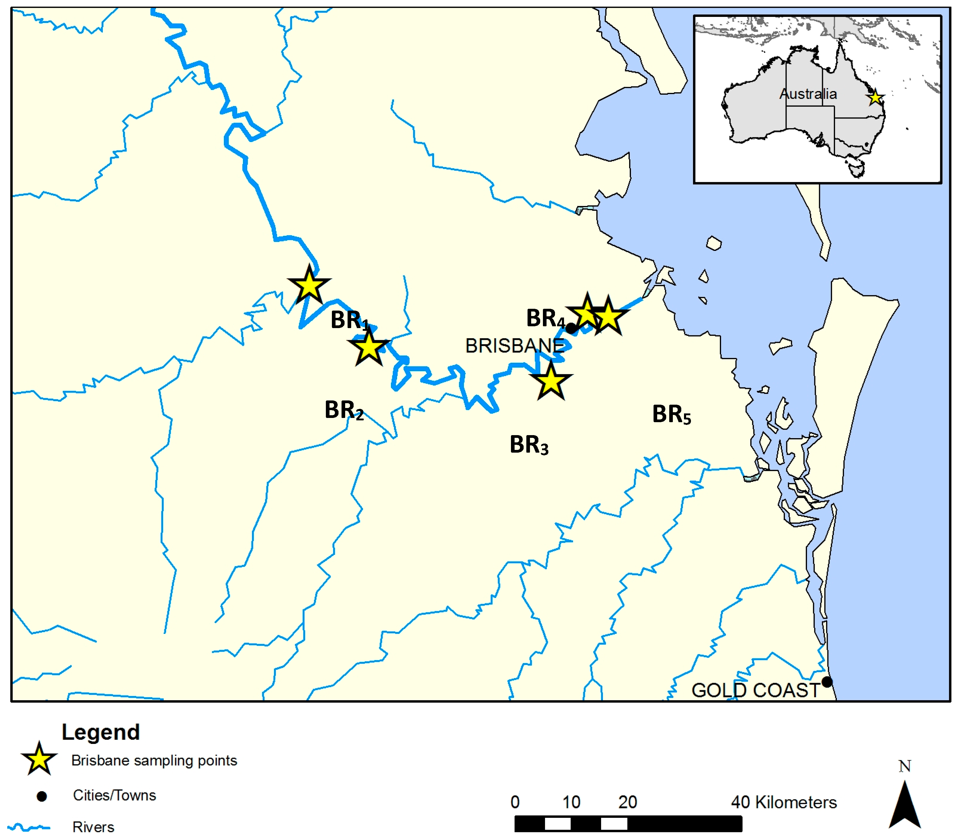
2.1. Water Sampling
2.2. Water Quality Analysis
2.2.1. Dissolved Organic Carbon
2.2.2. Trace Metals
2.2.3. Enumeration of Fecal Indicator Bacteria (FIB)
2.3. Biomass Collection from Water Samples
2.4. Metagenomic Analysis
2.4.1. DNA Extraction
2.4.2. PCR and Illumina MiSeq Sequencing
2.4.3. Sequence Data Analysis
2.5. Community Metabolomics Analysis
2.5.1. Sample Silyl Derivatization
2.5.2. Single Quadrupole GC-MS
2.6. Data Integration and Statistical Analysis
3. Results
3.1. Physico-Chemical Data
3.2. Trace Metals
3.3. Fecal Indicator Bacteria (FIB)
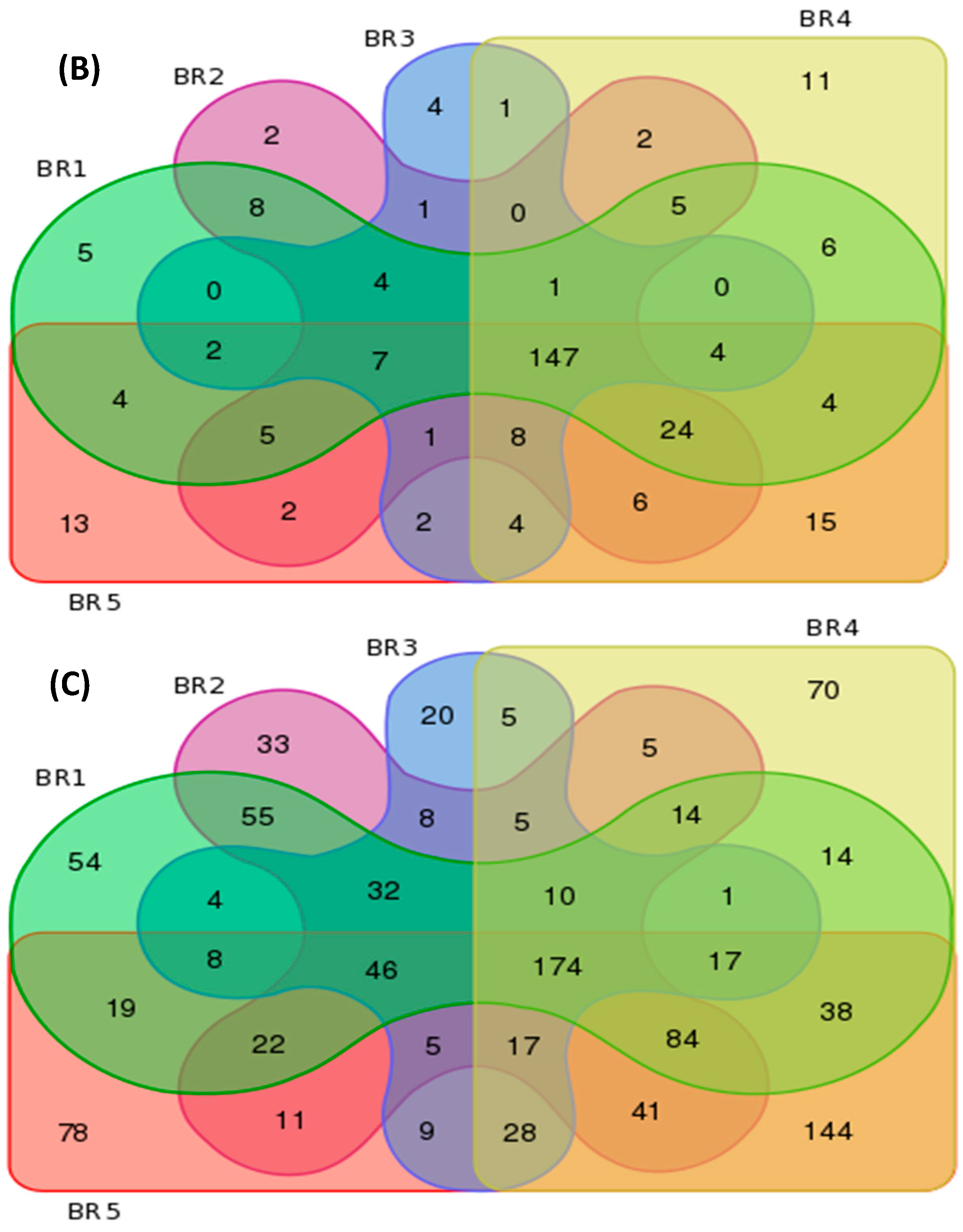
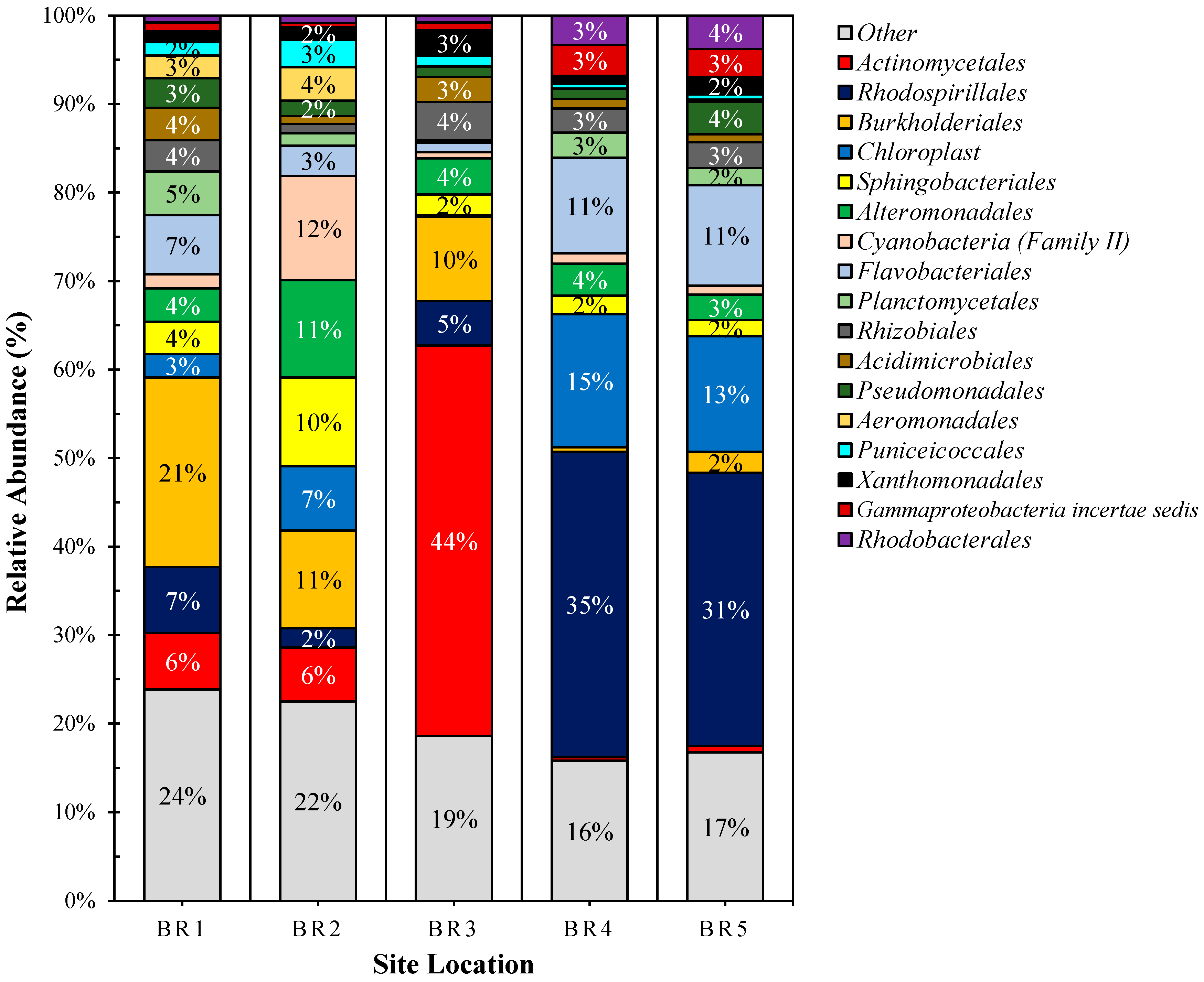
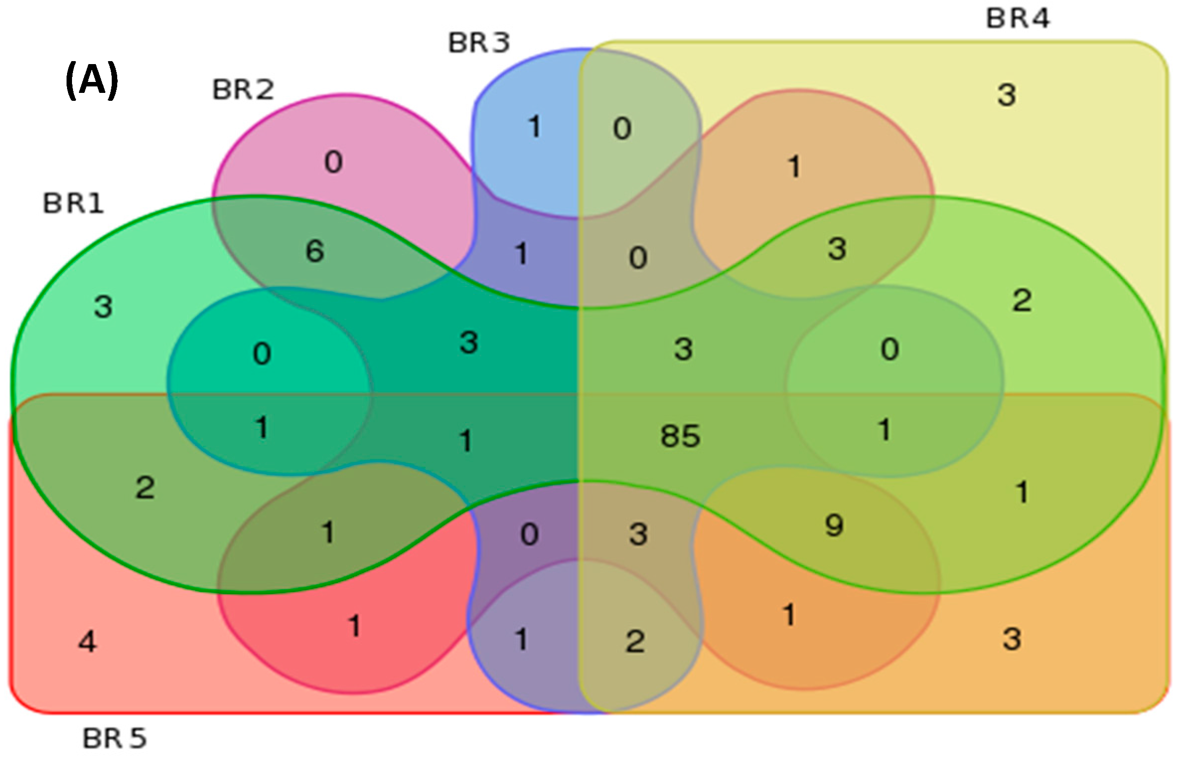
3.4. Metagenomics
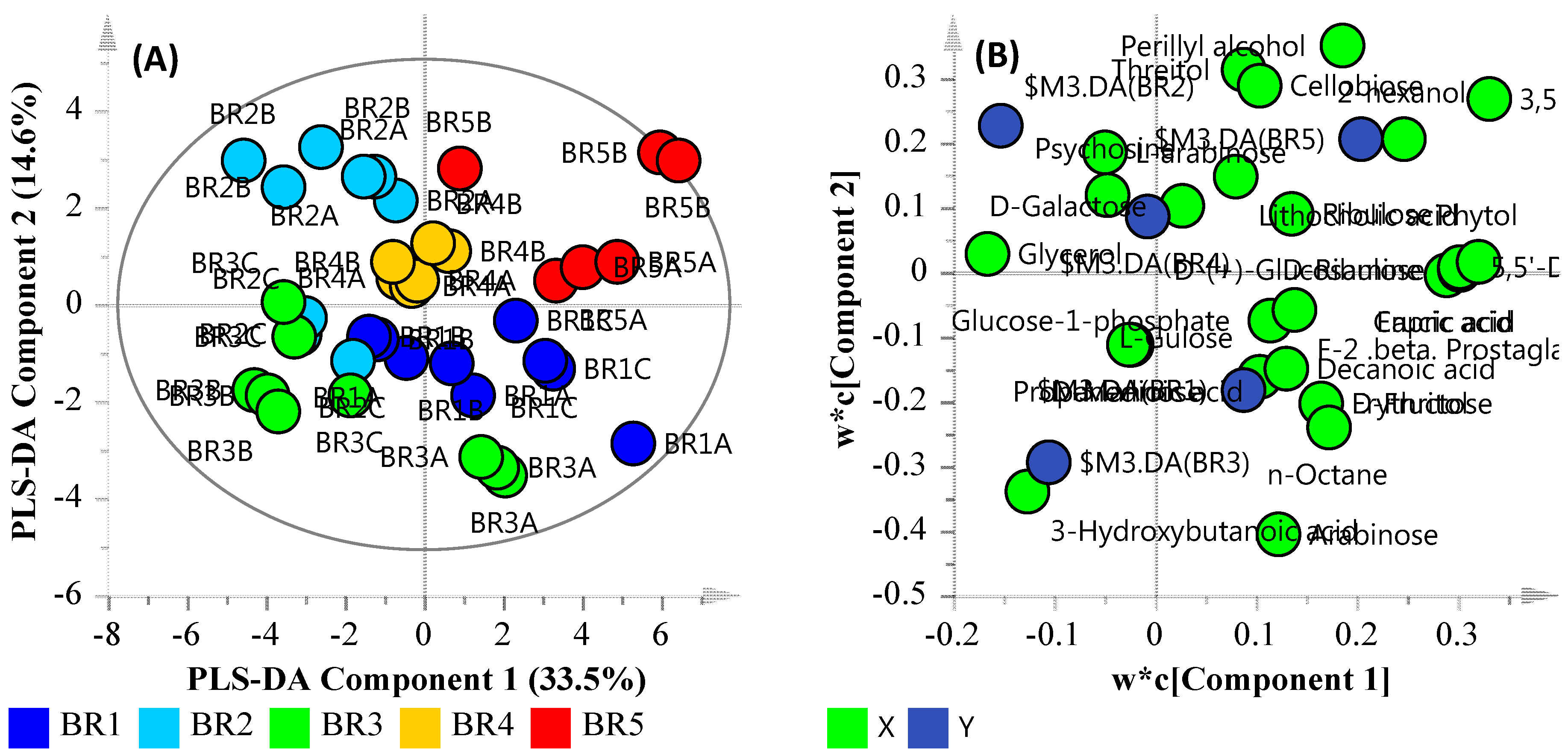
3.5. Community Metabolomics
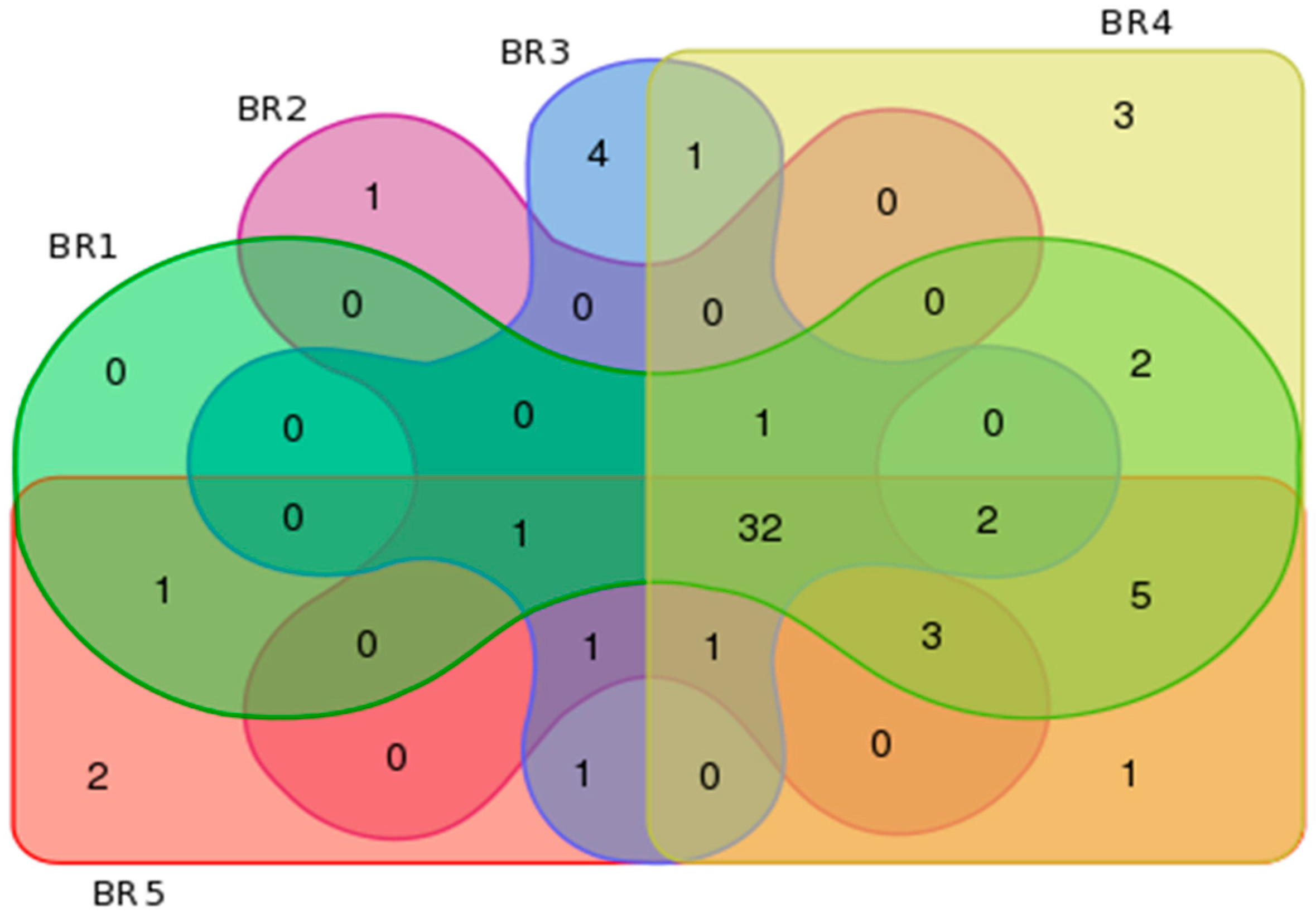
3.6. Multi-Omics
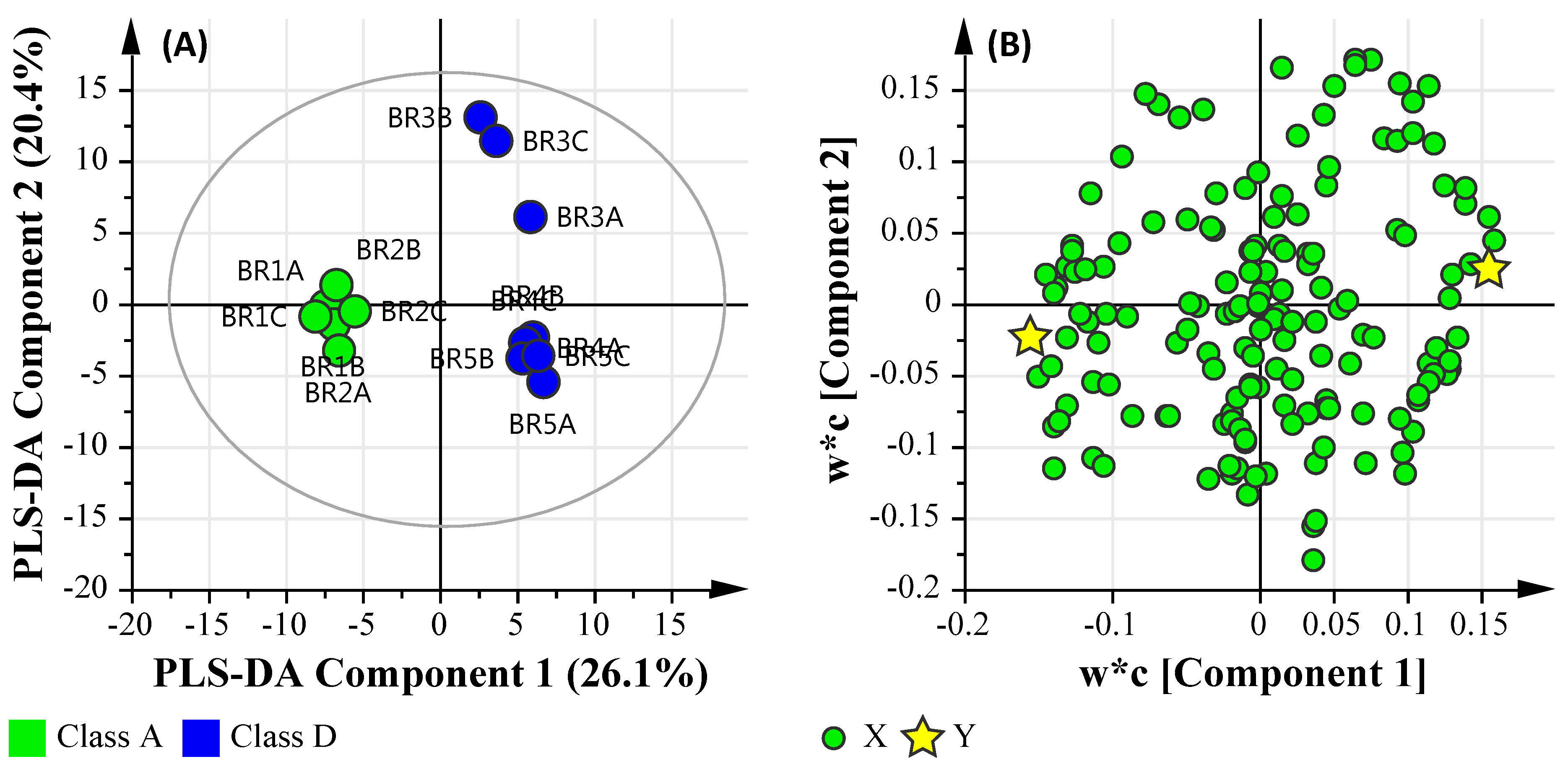
3.6.1. Microbial Water Quality Assessment Category Class Assessment
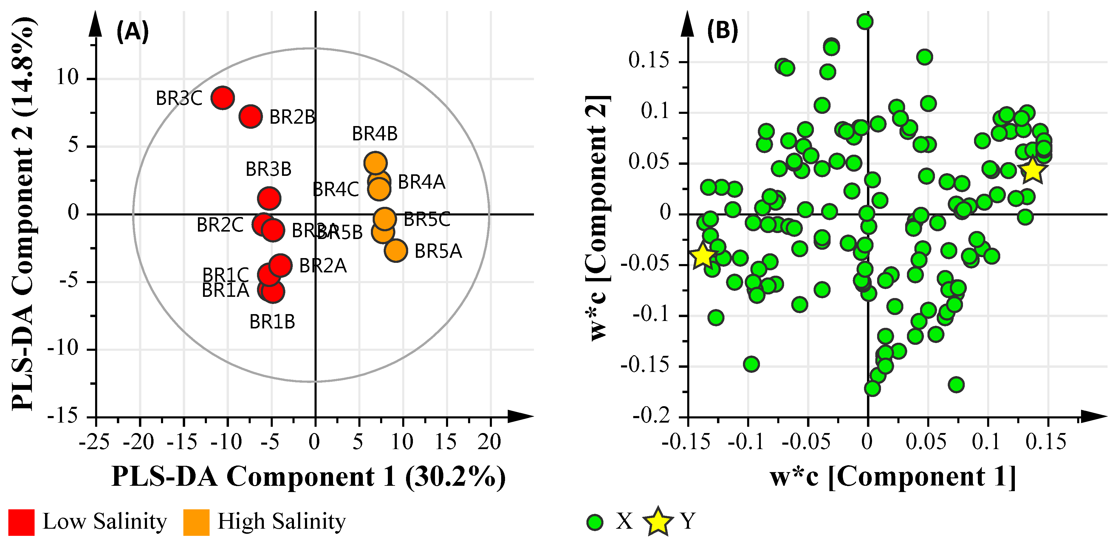
3.6.2. Salinity Assessment
3.6.3. Microbial Water Quality Assessment Category Class A and Low Salinity Assessment
4. Discussion
5. Conclusions
Acknowledgments
Author Contributions
Conflicts of Interest
References
- Abram, F. Systems-based approaches to unravel multi-species microbial community functioning. Comput. Struct. Biotechnol. J. 2015, 13, 24–32. [Google Scholar] [CrossRef] [PubMed]
- Robinson, A.M.; Gondalia, S.V.; Karpe, A.V.; Eri, R.; Beale, D.J.; Morrison, P.D.; Palombo, E.A.; Nurgali, K. Fecal microbiota and metabolome in a mouse model of spontaneous chronic colitis: Relevance to human inflammatory bowel disease. Inflamm. Bowel Dis. 2016, 22, 2767–2787. [Google Scholar] [CrossRef] [PubMed]
- Kumarasingha, R.; Karpe, A.V.; Preston, S.; Yeo, T.C.; Lim, D.S.L.; Tu, C.L.; Luu, J.; Simpson, K.J.; Shaw, J.M.; Gasser, R.B.; et al. Metabolic profiling and in vitro assessment of anthelmintic fractions of Picria fel-terrae Lour. Int. J. Parasitol. 2016, 6, 171–178. [Google Scholar] [CrossRef] [PubMed]
- Bundy, J.G.; Davey, M.P.; Viant, M.R. Environmental metabolomics: A critical review and future perspectives. Metabolomics 2009, 5, 3–21. [Google Scholar] [CrossRef]
- Hultman, J.; Waldrop, M.P.; Mackelprang, R.; David, M.M.; McFarland, J.; Blazewicz, S.J.; Harden, J.; Turetsky, M.R.; McGuire, A.D.; Shah, M.B.; et al. Multi-omics of permafrost, active layer and thermokarst bog soil microbiomes. Nature 2015, 521, 208–212. [Google Scholar] [CrossRef] [PubMed]
- Jones, O.A.H.; Sdepanian, S.; Lofts, S.; Svendsen, C.; Spurgeon, D.J.; Maguire, M.L.; Griffin, J.L. Metabolomic analysis of soil communities can be used for pollution assessment. Environ. Toxicol. Chem. 2014, 33, 61–64. [Google Scholar] [CrossRef] [PubMed]
- Desai, C.; Pathak, H.; Madamwar, D. Advances in molecular and “-omics” technologies to gauge microbial communities and bioremediation at xenobiotic/anthropogen contaminated sites. Bioresour. Technol. 2010, 101, 1558–1569. [Google Scholar] [CrossRef] [PubMed]
- Bullock, A.; Ziervogel, K.; Ghobrial, S.; Jalowska, A.; Arnosti, C. Microbial activities and organic matter degradation at three sites in the coastal North Atlantic: Variations in DOC turnover times and potential for export off the shelf. Mar. Chem. 2015, 177, 388–397. [Google Scholar] [CrossRef]
- Date, Y.; Nakanishi, Y.; Fukuda, S.; Kato, T.; Tsuneda, S.; Ohno, H.; Kikuchi, J. New monitoring approach for metabolic dynamics in microbial ecosystems using stable-isotope-labeling technologies. J. Biosci. Bioeng. 2010, 110, 87–93. [Google Scholar] [CrossRef] [PubMed]
- Hook, S.E.; Osborn, H.L.; Spadaro, D.A.; Simpson, S.L. Assessing mechanisms of toxicant response in the amphipod Melita plumulosa through transcriptomic profiling. Aquat. Toxicol. 2014, 146, 247–257. [Google Scholar] [CrossRef] [PubMed]
- Osborn, H.L.; Hook, S.E. Using transcriptomic profiles in the diatom Phaeodactylum tricornutum to identify and prioritize stressors. Aquat. Toxicol. 2013, 138–139, 12–25. [Google Scholar] [CrossRef] [PubMed]
- Llewellyn, C.A.; Sommer, U.; Dupont, C.L.; Allen, A.E.; Viant, M.R. Using community metabolomics as a new approach to discriminate marine microbial particulate organic matter in the western English Channel. Prog. Oceanogr. 2015, 137, 421–433. [Google Scholar] [CrossRef]
- Griffiths, W.J. Metabolomics, Metabonomics and Metabolite Profiling; Royal Society of Chemistry: Cambridge, UK, 2008. [Google Scholar]
- Harrigan, G.G.; Goodacre, R. Metabolic Profiling: Its Role in Biomarker Discovery and Gene Function Analysis; Springer Science & Business Media: New York, NY, USA, 2012. [Google Scholar]
- Lindon, J.C.; Holmes, E.; Nicholson, J.K. Metabonomics Techniques and Applications to Pharmaceutical Research & Development. Pharm. Res. 2006, 23, 1075–1088. [Google Scholar] [PubMed]
- Gómez-Canela, C.; Miller, T.H.; Bury, N.R.; Tauler, R.; Barron, L.P. Targeted metabolomics of Gammarus pulex following controlled exposures to selected pharmaceuticals in water. Sci. Total Environ. 2016, 562, 777–788. [Google Scholar] [CrossRef] [PubMed]
- Cao, C.; Wang, W.-X. Bioaccumulation and metabolomics responses in oysters Crassostrea hongkongensis impacted by different levels of metal pollution. Environ. Pollut. 2016, 216, 156–165. [Google Scholar] [CrossRef] [PubMed]
- Ji, C.; Yu, D.; Wang, Q.; Li, F.; Zhao, J.; Wu, H. Impact of metal pollution on shrimp Crangon affinis by NMR-based metabolomics. Mar. Pollut. Bull. 2016, 106, 372–376. [Google Scholar] [CrossRef] [PubMed]
- Thakur, N.L.; Jain, R.; Natalio, F.; Hamer, B.; Thakur, A.N.; Müller, W.E.G. Marine molecular biology: An emerging field of biological sciences. Biotechnol. Adv. 2008, 26, 233–245. [Google Scholar] [CrossRef] [PubMed]
- Kimes, N.E.; Callaghan, A.V.; Aktas, D.F.; Smith, W.L.; Sunner, J.; Golding, B.; Drozdowska, M.; Hazen, T.C.; Suflita, J.M.; Morris, P.J. Metagenomic analysis and metabolite profiling of deep–sea sediments from the Gulf of Mexico following the Deepwater Horizon oil spill. Front. Microbiol. 2013, 4, 50. [Google Scholar] [CrossRef] [PubMed]
- Yang, F.-C.; Chen, Y.-L.; Tang, S.-L.; Yu, C.-P.; Wang, P.-H.; Ismail, W.; Wang, C.-H.; Ding, J.-Y.; Yang, C.-Y.; Yang, C.-Y.; et al. Integrated multi-omics analyses reveal the biochemical mechanisms and phylogenetic relevance of anaerobic androgen biodegradation in the environment. ISME J. 2016, 10, 1967–1983. [Google Scholar] [CrossRef] [PubMed]
- Beale, D.J.; Karpe, A.V.; McLeod, J.D.; Gondalia, S.V.; Muster, T.H.; Othman, M.Z.; Palombo, E.A.; Joshi, D. An “omics” approach towards the characterisation of laboratory scale anaerobic digesters treating municipal sewage sludge. Water Res. 2016, 88, 346–357. [Google Scholar] [CrossRef] [PubMed]
- McLeod, J.D.; Othman, M.Z.; Beale, D.J.; Joshi, D. The use of laboratory scale reactors to predict sensitivity to changes in operating conditions for full-scale anaerobic digestion treating municipal sewage sludge. Bioresour. Technol. 2015, 189, 384–390. [Google Scholar] [CrossRef] [PubMed]
- Tan, B.; Ng, C.; Nshimyimana, J.P.; Loh, L.L.; Gin, K.Y.H.; Thompson, J.R. Next-generation sequencing (NGS) for assessment of microbial water quality: Current progress, challenges, and future opportunities. Front. Microbiol. 2015, 6, 1027. [Google Scholar] [CrossRef] [PubMed]
- Gomez-Alvarez, V.; Revetta, R.P.; Santo Domingo, J.W. Metagenomic Analyses of Drinking Water Receiving Different Disinfection Treatments. Appl. Environ. Microbiol. 2012, 78, 6095–6102. [Google Scholar] [CrossRef] [PubMed]
- Van Rossum, T.; Peabody, M.A.; Uyaguari-Diaz, M.I.; Cronin, K.I.; Chan, M.; Slobodan, J.R.; Nesbitt, M.J.; Suttle, C.A.; Hsiao, W.W.L.; Tang, P.K.C.; et al. Year-long metagenomic study of river microbiomes across land use and water quality. Front. Microbiol. 2015, 6, 1405. [Google Scholar] [CrossRef] [PubMed]
- Beale, D.J.; Barratt, R.; Marlow, D.R.; Dunn, M.S.; Palombo, E.A.; Morrison, P.D.; Key, C. Application of metabolomics to understanding biofilms in water distribution systems: A pilot study. Biofouling 2013, 29, 283–294. [Google Scholar] [CrossRef] [PubMed]
- Davis, J.M.; Ekman, D.R.; Teng, Q.; Ankley, G.T.; Berninger, J.P.; Cavallin, J.E.; Jensen, K.M.; Kahl, M.D.; Schroeder, A.L.; Villeneuve, D.L.; et al. Linking field-based metabolomics and chemical analyses to prioritize contaminants of emerging concern in the Great Lakes basin. Environ. Toxicol. Chem. 2016, 35, 2493–2502. [Google Scholar] [CrossRef] [PubMed]
- HealthyWaterways. 2012 Brisbane River Sitemap. Available online: http://healthywaterways.org/resources/documents/2012-brisbane-river-sitemap-doc-3476 (accessed on 3 November 2016).
- Oshiro, R.K. Method 1603: Escherichia coli (E. coli) in Water by Membrane Filtration Using Modified Membrane Thermotolerant Escherichia coli Agar (Modified mTEC); United States Environmental Protection Agency: Washington, DC, USA, 2002.
- Ahmed, W.; Stewart, J.; Powell, D.; Gardner, T. Evaluation of the host-specificity and prevalence of enterococci surface protein (esp) marker in sewage and its application for sourcing human fecal pollution. J. Environ. Qual. 2008, 37, 1583–1588. [Google Scholar] [CrossRef] [PubMed]
- Ahmed, W.; Sawant, S.; Huygens, F.; Goonetilleke, A.; Gardner, T. Prevalence and occurrence of zoonotic bacterial pathogens in surface waters determined by quantitative PCR. Water Res. 2009, 43, 4918–4928. [Google Scholar] [CrossRef] [PubMed]
- Ahmed, W.; Staley, C.; Sadowsky, M.J.; Gyawali, P.; Sidhu, J.P.S.; Palmer, A.; Beale, D.J.; Toze, S. Toolbox approaches using molecular markers and 16S rRNA gene amplicon data sets for identification of fecal pollution in surface water. Appl. Environ. Microbiol. 2015, 81, 7067–7077. [Google Scholar] [CrossRef] [PubMed]
- Claesson, M.J.; Wang, Q.; O’Sullivan, O.; Greene-Diniz, R.; Cole, J.R.; Ross, R.P.; O’Toole, P.W. Comparison of two next-generation sequencing technologies for resolving highly complex microbiota composition using tandem variable 16S rRNA gene regions. Nucleic Acids Res. 2010, 38, e200. [Google Scholar] [CrossRef] [PubMed]
- Youssef, N.; Sheik, C.S.; Krumholz, L.R.; Najar, F.Z.; Roe, B.A.; Elshahed, M.S. Comparison of species richness estimates obtained using nearly complete fragments and simulated pyrosequencing-generated fragments in 16S rRNA gene-based environmental surveys. Appl. Environ. Microbiol. 2009, 75, 5227–5236. [Google Scholar] [CrossRef] [PubMed]
- Schloss, P.D.; Westcott, S.L.; Ryabin, T.; Hall, J.R.; Hartmann, M.; Hollister, E.B.; Lesniewski, R.A.; Oakley, B.B.; Parks, D.H.; Robinson, C.J. Introducing mothur: Open-source, platform-independent, community-supported software for describing and comparing microbial communities. Appl. Environ. Microbiol. 2009, 75, 7537–7541. [Google Scholar] [CrossRef] [PubMed]
- Aronesty, E. Comparison of sequencing utility programs. Open Bioinforma. J. 2013, 7, 1–8. [Google Scholar] [CrossRef]
- Pruesse, E.; Quast, C.; Knittel, K.; Fuchs, B.M.; Ludwig, W.; Peplies, J.; Glöckner, F.O. SILVA: A comprehensive online resource for quality checked and aligned ribosomal RNA sequence data compatible with ARB. Nucleic Acids Res. 2007, 35, 7188–7196. [Google Scholar] [CrossRef] [PubMed]
- Huse, S.M.; Welch, D.M.; Morrison, H.G.; Sogin, M.L. Ironing out the wrinkles in the rare biosphere through improved OTU clustering. Environ. Microbiol. 2010, 12, 1889–1898. [Google Scholar] [CrossRef] [PubMed]
- Kunin, V.; Engelbrektson, A.; Ochman, H.; Hugenholtz, P. Wrinkles in the rare biosphere: Pyrosequencing errors can lead to artificial inflation of diversity estimates. Environ. Microbiol. 2010, 12, 118–123. [Google Scholar] [CrossRef] [PubMed]
- Edgar, R.C.; Haas, B.J.; Clemente, J.C.; Quince, C.; Knight, R. UCHIME improves sensitivity and speed of chimera detection. Bioinformatics 2011, 27, 2194–2200. [Google Scholar] [CrossRef] [PubMed]
- Cole, J.R.; Wang, Q.; Cardenas, E.; Fish, J.; Chai, B.; Farris, R.J.; Kulam-Syed-Mohideen, A.; McGarrell, D.M.; Marsh, T.; Garrity, G.M. The Ribosomal Database Project: Improved alignments and new tools for rRNA analysis. Nucleic Acids Res. 2009, 37, D141–D145. [Google Scholar] [CrossRef] [PubMed]
- Karpe, A.V.; Beale, D.J.; Godhani, N.B.; Morrison, P.D.; Harding, I.H.; Palombo, E.A. Untargeted metabolic profiling of winery-derived biomass waste degradation by Penicillium chrysogenum. J. Agric. Food Chem. 2015, 63, 10696–10704. [Google Scholar] [CrossRef] [PubMed]
- Beale, D.; Morrison, P.; Key, C.; Palombo, E. Metabolic profiling of biofilm bacteria known to cause microbial influenced corrosion. Water Sci. Technol. 2014, 69, 1–8. [Google Scholar] [CrossRef] [PubMed]
- Beale, D.J.; Marney, D.; Marlow, D.R.; Morrison, P.D.; Dunn, M.S.; Key, C.; Palombo, E.A. Metabolomic analysis of Cryptosporidium parvum oocysts in water: A proof of concept demonstration. Environ. Pollut. 2013, 174, 201–203. [Google Scholar] [CrossRef] [PubMed]
- Karpe, A.V.; Beale, D.J.; Morrison, P.D.; Harding, I.H.; Palombo, E.A. Untargeted metabolic profiling of vitis vinifera during Fungal Degradation. FEMS Microbiol. Lett. 2015. [Google Scholar] [CrossRef] [PubMed]
- Karpe, A.; Beale, D.; Godhani, N.; Morrison, P.; Harding, I.; Palombo, E. Untargeted metabolic profiling of winery-derived biomass waste degradation by Aspergillus niger. J. Chem. Technol. Biotechnol. 2015, 197, 1–12. [Google Scholar]
- Fiehn, O.; Robertson, D.; Griffin, J.; van der Werf, M.; Nikolau, B.; Morrison, N.; Sumner, L.W.; Goodacre, R.; Hardy, N.W.; Taylor, C. The metabolomics standards initiative (MSI). Metabolomics 2007, 3, 175–178. [Google Scholar] [CrossRef]
- Australian Water Association (AWA). Australian and New Zealand Guidelines for Fresh and Marine Water Quality. Volume 1, The Guidelines; Australian and New Zealand Environment and Conservation Council, Agriculture and Resource Management Council of Australia and New Zealand: Artarmon, Sydney, Australia, 2000.
- Ahmed, W.; Sidhu, J.P.S.; Toze, S. Evaluation of the nifH gene marker of methanobrevibacter smithii for the detection of sewage pollution in environmental waters in southeast Queensland, Australia. Environ. Sci. Technol. 2012, 46, 543–550. [Google Scholar] [CrossRef] [PubMed]
- Ahmed, W.; Powell, D.; Goonetilleke, A.; Gardner, T. Detection and source identification of faecal pollution in non-sewered catchment by means of host-specific molecular markers. Water Sci. Technol. 2008, 58, 579–586. [Google Scholar] [CrossRef] [PubMed]
- Ahmed, W.; Sidhu, J.P.S.; Smith, K.; Beale, D.J.; Gyawali, P.; Tozea, S. Distributions of fecal markers in wastewater from different climatic zones for human fecal pollution tracking in Australian surface waters. Appl. Environ. Microbiol. 2016, 82, 1316–1323. [Google Scholar] [CrossRef] [PubMed]
- EHMP, Ecosystem Health Monitoring Program 2005–2006 Annual Technical Report. Available online: http://www.ehmp.org/media/scripts/doc_download.aspx?did=721 (accessed on 15 June 2007).
- Cheng, T.-C.; DeFrank, J.J.; Rastogi, V.K. Alteromonas prolidase for organophosphorus G-agent decontamination. Chem. Biol. Interact. 1999, 119–120, 455–462. [Google Scholar] [CrossRef]
- Huang, L.; Gao, X.; Liu, M.; Du, G.; Guo, J.; Ntakirutimana, T. Correlation among soil microorganisms, soil enzyme activities, and removal rates of pollutants in three constructed wetlands purifying micro-polluted river water. Ecol. Eng. 2012, 46, 98–106. [Google Scholar] [CrossRef]
- Jeong, J.-Y.; Park, H.-D.; Lee, K.-H.; Weon, H.-Y.; Ka, J.-O. Microbial community analysis and identification of alternative host-specific fecal indicators in fecal and river water samples using pyrosequencing. J. Microbiol. 2011, 49, 585. [Google Scholar] [CrossRef] [PubMed]
- Xue, Q.; Shimizu, K.; Sakharkar, M.K.; Utsumi, M.; Cao, G.; Li, M.; Zhang, Z.; Sugiura, N. Geosmin degradation by seasonal biofilm from a biological treatment facility. Environ. Sci. Pollut. Res. 2012, 19, 700–707. [Google Scholar] [CrossRef] [PubMed]
- Yu, J.; Li, Y.; Han, G.; Zhou, D.; Fu, Y.; Guan, B.; Wang, G.; Ning, K.; Wu, H.; Wang, J. The spatial distribution characteristics of soil salinity in coastal zone of the Yellow River Delta. Environ. Earth Sci. 2014, 72, 589–599. [Google Scholar] [CrossRef]
- Shakilabanu, S. Biodiversity of plant growth promoting rhizobacteria in mangrove ecosystem—A review. Int. J. Pharm. Biol. Arch. 2012, 3, 3. [Google Scholar]
- Yoneda, S.; Kawarai, T.; Narisawa, N.; Tuna, E.B.; Sato, N.; Tsugane, T.; Saeki, Y.; Ochiai, K.; Senpuku, H. Effects of short-chain fatty acids on Actinomyces naeslundii biofilm formation. Mol. Oral Microbiol. 2013, 28, 354–365. [Google Scholar] [CrossRef] [PubMed]
- Ylla, I.; Canhoto, C.; Romaní, A.M. Effects of Warming on Stream Biofilm Organic Matter Use Capabilities. Microb. Ecol. 2014, 68, 132–145. [Google Scholar] [CrossRef] [PubMed]
- Chandra, R.; Arora, S.; Rohit, M.V.; Venkata Mohan, S. Lipid metabolism in response to individual short chain fatty acids during mixotrophic mode of microalgal cultivation: Influence on biodiesel saturation and protein profile. Bioresour. Technol. 2015, 188, 169–176. [Google Scholar] [CrossRef] [PubMed]


| BR Site | EHMP Site | GPS Coordinates | Temp. (°C) | Conductivity (mS·cm−1) | Salinity (ppt) | pH | Turbidity (NTU) | DOC * (mg·L−1) | Site Characteristics | Suspected Source of Pollution |
|---|---|---|---|---|---|---|---|---|---|---|
| BR1 | 714 | 27°23′58” S; 152°36′26′′ E | 21.7 (0.4) | 0.39 (<0.1) | 0.19 (<0.1) | 7.14 (<0.1) | 0.5 (1.7) | 9.32 (0.8) | Rural | Wildlife, waterfowl, recreational activities. |
| BR2 | 711 | 27°29′51′′ S; 152°42′7′′ E | 28.1 (<0.1) | 0.53 (<0.1) | 0.25 (<0.1) | 8.00 (<0.1) | 5.2 (0.1) | 9.30 (0.4) | Rural | Cattle, horses, septic tanks, wildlife. |
| BR3 | 718 | 27°33′8′′ S; 152°59′31′′ E | 26.6 (<0.1) | 0.7 (<0.1) | 0.32 (<0.1) | 7.00 (<0.1) | 137 (0.2) | 8.88 (0.5) | Peri urban, tidally influenced | Wastewater treatment plants, waterfowls. |
| BR4 | 703 | 27°26′38′′ S; 153°3′3′′ E | 25.7 (<0.1) | 46.5 (<0.1) | 30.17 (<0.1) | 7.77 (<0.1) | 15.3 (4.4) | 4.35 (0.5) | Urban | Recreational activities, tidal influence. |
| BR5 | 702 | 27°26′56′′ S; 153°5′0′′ E | 25.4 (<0.1) | 46.9 (<0.13) | 30.47 (0.3) | 7.71 (<0.1) | 11.6 (0.1) | 5.02 (1.2) | Urban | Port, industrial activities, tidal influence. |
| BR Site | EHMP Site | Chlorophyll a (μg·L−1) | Light Penetration (Secchi Depth, m) | Phosphorus as P | Nitrogen as N | ||||
|---|---|---|---|---|---|---|---|---|---|
| FRP * (μg·L−1) | Total (μg·L−1) | Ammonia (μg·L−1) | Organic (μg·L−1) | Oxides (μg·L−1) | Total (μg·L−1) | ||||
| BR1 | 714 | 6.30 | 0.45 | 31 | 61 | <4 | 323 | 13 | 340 |
| BR2 | 711 | 0.37 | 0.15 | 240 | 320 | 12 | 368 | 500 | 880 |
| BR3 | 718 | 1.50 | 0.60 | 260 | 270 | 6 | 254 | 550 | 810 |
| BR4 | 703 | 2.24 | 0.50 | 93 | 140 | 8 | 202 | 210 | 420 |
| BR5 | 702 | 2.13 | 0.85 | 64 | 79 | 10 | 190 | 100 | 300 |
| BR Site | Concentration of Metals (RSD %) | ||||||||
|---|---|---|---|---|---|---|---|---|---|
| Aluminum (Al, ng·L−1) | Cadmium (Cd, ng·L−1) | Cobalt (Co, ng·L−1) | Chromium (Cr, ng·L−1) | Copper (Cu, ng·L−1) | Iron (Fe, ng·L−1) | Lead (Pb, ng·L−1) | Nickel (Ni, ng·L−1) | Zinc (Zn, ng·L−1) | |
| BR1 | 1.0 (>0.1) | <0.04 | 0.04 (4.7) | <0.02 | 3.0 (0.1) | <0.571 | <0.06 | <0.06 | 4.6 (2.3) |
| BR2 | 1.0 (>0.1) | <0.04 | 0.14 (5.3) | <0.02 | 3.1 (0.1) | 32.0 (3.0) | <0.06 | 0.2 (0.1) | 3.6 (0.6) |
| BR3 | 2008 (4.9) | <0.04 | 2.38 (2.4) | 1.0 (0.1) | 8.1 (0.1) | 4529.7 (188.1) | 7.6 (0.2) | 2.8 (0.1) | 36.9 (1.2) |
| BR4 | 1.0 (>0.1) | <0.04 | 0.15 (10.1) | <0.02 | 4.3 (0.6) | 94.1 (59.3) | <0.06 | 0.4 (0.2) | 6.2 (3.1) |
| BR5 | 11.0 (1.9) | <0.04 | 0.26 (3.4) | <0.02 | 4.0 (0.2) | 234.7 (27.6) | <0.06 | 0.4 (0.1) | 6.8 (1.5) |
| BR Site | Fecal Indicator Bacteria (FIB) a | Recreational Microbial Water Quality Assessment b | ||||
|---|---|---|---|---|---|---|
| E. coli/100 mL Geometric Mean (Std. Dev.) | Enterococcus spp./100 mL Geometric Mean (Std. Dev.) | Enterococcus spp. (<33 CFU/100 mL (%)) | Enterococcus spp. (>157 CFU/100 mL (%)) | Standardized (95th Percentile c) | Microbial Water Quality Assessment Category (MAC) | |
| BR1 | 15 (4) | 4 (2) | 100 | 0 | 2 | A |
| BR2 | 69 (18) | 22 (5) | 100 | 0 | 2 | A |
| BR3 | 307 (49) | 544 (85) | 0 | 100 | 13,300 | D |
| BR4 | 149 (25) | 189 (24) | 0 | 89 | 12,900 | D |
| BR5 | 88 (16) | 163 (37) | 0 | 56 | 10,600 | D |
| BR Sites | Features per Group | Unique Features per Site | ||||
|---|---|---|---|---|---|---|
| Order | Family | Genus | Order | Family | Genus | |
| BR1 | 121 | 226 | 592 | 3 | 5 | 54 |
| BR2 | 118 | 223 | 562 | 0 | 2 | 33 |
| BR3 | 102 | 186 | 389 | 1 | 4 | 20 |
| BR4 | 117 | 238 | 667 | 3 | 11 | 70 |
| BR5 | 116 | 248 | 741 | 4 | 13 | 78 |
| Compound | Description | Fold Change | p-Value | Adj. p-Value |
|---|---|---|---|---|
| l-Gulose (5TMS) | Monosaccharide sugar | 2.885793773 | 3.60 × 10⁻⁶ | 5.00 × 10⁻² |
| l-Arabinose (4TMS) | Sugar | 1.995251285 | 0.20237 | 3.82 × 10⁻² |
| Glycerol (3TMS) | Component of triglycerides and of phospholipids | 1.850174576 | 0.41024 | 3.13 × 10⁻² |
| α-d-Glucose-1-phosphate, dipotassium salt dihydrate | 1.792927932 | 0.85638 | 9.72 × 10⁻³ | |
| Psychosine sulfate (dTMS) | Lipid and intermediate in the biosynthesis of cerebrosides | 1.744904803 | 0.049444 | 4.58 × 10⁻² |
| d-Cellobiose (1MEOX, 8TMS) | Disaccharide sugar | 1.626482976 | 0.0061321 | 4.86 × 10⁻² |
| 2-methyl-2-butenedioic acid (2TMS) | Carboxylic acid | 1.535874614 | 0.4597 | 2.71 × 10⁻² |
| Prostaglandin F2β (1MEOX, 4TMS) | Arachidonic acid metabolites | 1.196188199 | 0.1738 | 3.96 × 10⁻² |
| d-Threitol (4TMS) | End product of d-xylose metabolism | 1.092677384 | 0.60615 | 1.74 × 10⁻² |
| d-Fructose (5TMS) | Monosaccharide sugar | 1.041734383 | 0.4944 | 2.08 × 10⁻² |
| n-Octane | Component of Fatty acid metabolism | 0.981496334 | 0.92237 | 3.47 × 10⁻³ |
| Perillyl alcohol (dTMS) | Isolated from the essential oils | 0.959935677 | 0.60615 | 1.67 × 10⁻² |
| Decanoic acid methyl ester (1TMS) | Constituent of many plants | 0.956956828 | 0.44286 | 2.85 × 10⁻² |
| d-Arabinose (4TMS) | Intermediate in biosynthesis of lipopolysaccharide | 0.893785022 | 0.41024 | 3.06 × 10⁻² |
| l-Tyrosine (3TMS) | Amino acid | 0.834176724 | 0.87829 | 6.94 × 10⁻³ |
| Erucic acid methyl ester (1TMS) | Fatty acids | 0.790950415 | 0.11213 | 4.17 × 10⁻² |
| Capric acid (1TMS) | Fatty acids | 0.790934596 | 0.11213 | 4.24 × 10⁻² |
| d-Glucose 6-phosphate (1MEOX, 6TMS) | Aminosaccharide | 0.782548013 | 0.07339 | 4.44 × 10⁻² |
| Phytol (1TMS) | Constituent of chlorophyll | 0.706423756 | 0.034756 | 4.65 × 10⁻² |
| Unknown Compound 10 (MW = 206.2) | 0.662675401 | 0.2944 | 3.47 × 10⁻² | |
| Erythritol (4TMS) | Sugar alcohol | 0.659587922 | 0.24544 | 3.75 × 10⁻² |
| 3,6-anhydro-d-Galactose (dTMS) | 0.6094551 | 0.088429 | 4.38 × 10⁻² | |
| d-Ribulose (1MEOX, 4TMS) | Monosaccharide sugar | 0.317429352 | 0.014781 | 4.72 × 10⁻² |
| d-Mannose (dTMS) | Carbohydrate | 0.27712129 | 0.58678 | 1.81 × 10⁻² |
| Lithocholic acid (2TMS) | Bile acid formed from chenodeoxycholate by bacterial action | 0.203416434 | 0.58678 | 1.88 × 10⁻² |
| Butanoic acid methyl ester (1TMS) | Fatty acid methyl ester | 0.153370303 | 0.96669 | 2.78 × 10⁻³ |
| 2-methylpropanedioic acid (2TMS) | Malonic acid derivative | 0.152544336 | 0.34935 | 3.33 × 10⁻² |
| BR Site | Monitoring Indicators | |||||||||||||
|---|---|---|---|---|---|---|---|---|---|---|---|---|---|---|
| Physico-Chemical | Microbial | |||||||||||||
| Salinity | Turbidity | pH | Cholorphyll a | TP | FRP | TN | NOx | NH4+ | Metals | E. coli | Enterococcus spp. | FIB (combined) | MAC * | |
| BR1 | N | N | N | Y | Y | Y | N | N | N | N | L | L | N | A |
| BR2 | N | N | N | N | Y | Y | Y | Y | N | N | L | L | N | A |
| BR3 | N | Y | N | N | Y | Y | Y | Y | N | N | H | H | Y | D |
| BR4 | Y | Y | N | N | Y | Y | N | Y | N | N | H | H | Y | D |
| BR5 | Y | Y | N | N | Y | Y | N | Y | N | N | H | H | Y | D |
© 2017 by the authors. Licensee MDPI, Basel, Switzerland. This article is an open access article distributed under the terms and conditions of the Creative Commons Attribution (CC BY) license ( http://creativecommons.org/licenses/by/4.0/).
Share and Cite
Beale, D.J.; Karpe, A.V.; Ahmed, W.; Cook, S.; Morrison, P.D.; Staley, C.; Sadowsky, M.J.; Palombo, E.A. A Community Multi-Omics Approach towards the Assessment of Surface Water Quality in an Urban River System. Int. J. Environ. Res. Public Health 2017, 14, 303. https://doi.org/10.3390/ijerph14030303
Beale DJ, Karpe AV, Ahmed W, Cook S, Morrison PD, Staley C, Sadowsky MJ, Palombo EA. A Community Multi-Omics Approach towards the Assessment of Surface Water Quality in an Urban River System. International Journal of Environmental Research and Public Health. 2017; 14(3):303. https://doi.org/10.3390/ijerph14030303
Chicago/Turabian StyleBeale, David J., Avinash V. Karpe, Warish Ahmed, Stephen Cook, Paul D. Morrison, Christopher Staley, Michael J. Sadowsky, and Enzo A. Palombo. 2017. "A Community Multi-Omics Approach towards the Assessment of Surface Water Quality in an Urban River System" International Journal of Environmental Research and Public Health 14, no. 3: 303. https://doi.org/10.3390/ijerph14030303
APA StyleBeale, D. J., Karpe, A. V., Ahmed, W., Cook, S., Morrison, P. D., Staley, C., Sadowsky, M. J., & Palombo, E. A. (2017). A Community Multi-Omics Approach towards the Assessment of Surface Water Quality in an Urban River System. International Journal of Environmental Research and Public Health, 14(3), 303. https://doi.org/10.3390/ijerph14030303