
Air Quality and Health Impacts of Future Ethanol Production and Use in São Paulo State, Brazil


 ,
,
Abstract
:1. Introduction
2. Materials and Methods
2.1. Emissions
2.1.1. Emissions from Sugarcane Straw Burning
2.1.2. Vehicle Emissions
2.1.3. Other Emissions
2.2. Air Quality Modeling
2.3. Health Impact Calculations
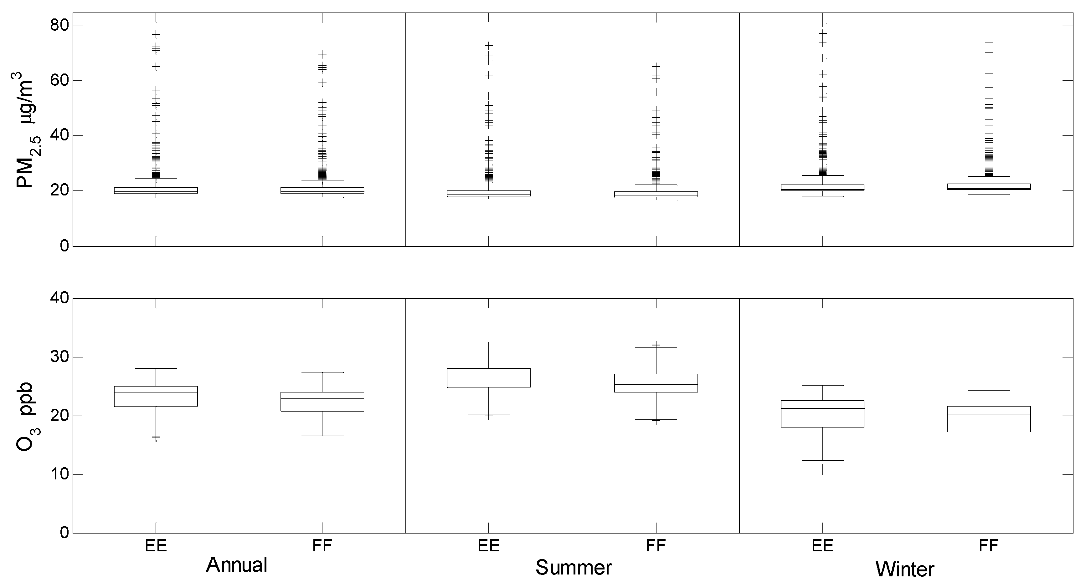
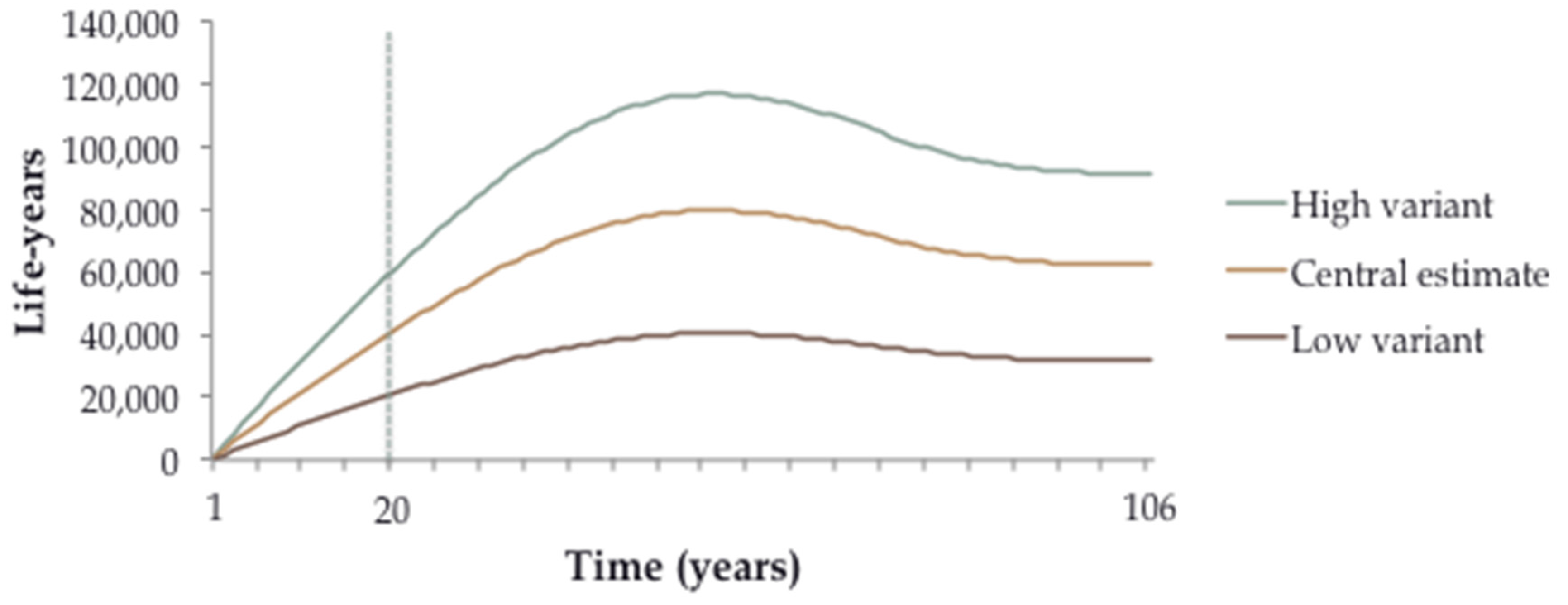
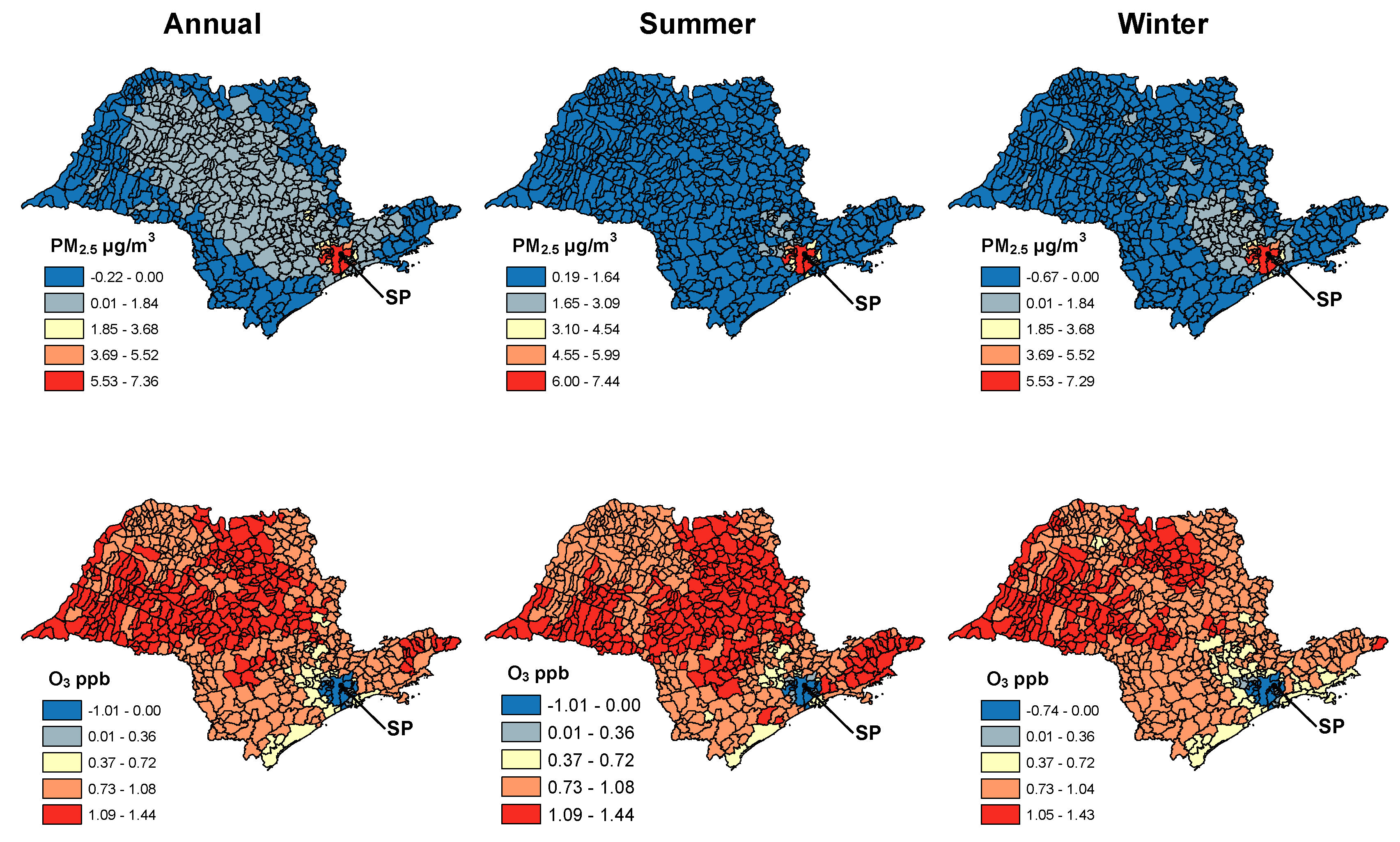
3. Results
4. Discussion
5. Conclusions
Supplementary Materials
Acknowledgments
Author Contributions
Conflicts of Interest
Abbreviations
| CCATT-BRAMS | Coupled Chemistry Aerosol and Tracer Transport model to the Brazilian developments on the Regional Atmospheric Modeling System |
| CI | Confidence interval |
| EE | Ethanol Expansion (scenario) |
| FF | Fossil Fuel (scenario) |
| MW | Megawatt |
| NOx | oxides of nitrogen |
| PM2.5 | Fine particulate matter |
| VOC | Volatile organic compound |
| WHO | World Health Organization |
References
- Renewable Fuels Association. World Fuel Ethanol Production. Available online: http://www.ethanolrfa.org/resources/industry/statistics/-1454098996479-8715d404-e546 (accessed on 11 February 2016).
- International Energy Agency. World Energy Outlook 2014; IEA/OECD: Paris, France, 2014. [Google Scholar]
- REN21. Renewables Global Futures Report; REN21: Paris, France, 2014. [Google Scholar]
- Renewable Fuels Association. Ethanol Facts: Environment. Available online: http://www.ethanolrfa.org/pages/ethanol-facts-environment (accessed on 7 January 2014).
- UNICA and Apex Brasil. Sugarcane Benefits: Improved Public Health. Available online: http://sugarcane.org/sugarcane-benefits/improved-public-health (accessed on 7 January 2014).
- Anderson, L.G. Effects of biodiesel fuels use on vehicle emissions. J. Sustain. Energy Environ. 2012, 3, 35–47. [Google Scholar]
- Niven, R. Ethanol in gasoline: Environmental impacts and sustainability review article. Renew. Sustain. Energy Rev. 2005, 9, 535–555. [Google Scholar] [CrossRef]
- Tessum, C.; Marshall, J.D.; Hill, J. Tank to Wheel Emissions of Ethanol and Biodiesel Powered Vehicles as Compared to Petroleum Alternatives; Center for Transportation Studies, University of Minnesota: Minneapolis, MN, USA, 2010; p. 10. [Google Scholar]
- Scovronick, N.; Wilkinson, P. Health impacts of liquid biofuel production and use: A review. Glob. Environ. Chang. 2014, 24, 155–164. [Google Scholar] [CrossRef]
- Wallington, T.; Anderson, J.; Kurtz, E.; Tennison, P. Biofuels, vehicle emissions and urban air quality. Faraday Discuss. 2016. [Google Scholar] [CrossRef] [PubMed]
- Goldemberg, J.; Coelho, S.; Guardabassi, P. The sustainability of ethanol production from sugarcane. Energy Policy 2008, 36, 2086–2097. [Google Scholar] [CrossRef]
- ANFAVEA. Anuário da Indústria Automobilística Brasileira 2014; ANFAVEA: São Paulo, Brazil, 2014. [Google Scholar]
- Empresa de Pesquisa Energética. Balanço Energético Nacional 2014; EPE: Rio de Janeiro, Brazil, 2014. [Google Scholar]
- UNICA. How Important Is Sugarcane to Meeting Brazil’s Energy Needs? Available online: http://www.unica.com.br/faq/ (accessed on 12 February 2016).
- UNICA. Unicadata. Available online: http://www.unicadata.com.br/historico-de-producao-e-moagem.php?idMn = 31&tipoHistorico = 2 (accessed on 11 February 2016).
- Arbex, M.; Bohm, G.; Saldiva, P.; Conceiçao, G.; Pope, A.; Braga, A. Assessment of the effects of sugar cane plantation burning on daily counts of inhalation therapy. J. Air Waste Manag. Assoc. 2000, 50, 1745–1749. [Google Scholar] [CrossRef] [PubMed]
- Arbex, M.; Martins, L.; de Oliveira, R.; Pereira, L.; Arbex, F.; Cancado, J.; Saldiva, P.; Braga, A. Air pollution from biomass burning and asthma hospital admissions in a sugar cane plantation area in brazil. J. Epidemiol. Community Health 2007, 61, 395–400. [Google Scholar] [CrossRef] [PubMed]
- Cançado, J.; Saldiva, P.; Pereira, L.; Lara, L.; Artaxo, P.; Martinelli, L.; Arbex, M.; Zanobetti, A.; Braga, A. The impact of sugar cane-burning emissions on the respiratory system of children and the elderly. Environ. Health Perspect. 2006, 114, 725–729. [Google Scholar] [CrossRef] [PubMed] [Green Version]
- Goto, D.M.; Lanca, M.; Obuti, C.A.; Galvao Barbosa, C.M.; Nascimento Saldiva, P.H.; Trevisan Zanetta, D.M.; Lorenzi-Filho, G.; de Paula Santos, U.; Nakagawa, N.K. Effects of biomass burning on nasal mucociliary clearance and mucus properties after sugarcane harvesting. Environ. Res. 2011, 111, 664–669. [Google Scholar] [CrossRef] [PubMed]
- World Health Organizaton. Ambient (Outdoor) Air Pollution in Cities Database 2014. Available online: http://www.who.int/phe/health_topics/outdoorair/databases/cities/en/ (accessed on 11 February 2016).
- World Health Organizaton. Who Air Quality Guidelines for Particulate Matter, Ozone, Nitrogen Dioxide and Sulfur Dioxide: Global Update 2005; WHO: Geneva, Switzerland, 2006. [Google Scholar]
- Empresa de Pesquisa Energética. Plano Nacional de Energia 2030; MME/EPE: Rio de Janeiro, Brazil, 2007. [Google Scholar]
- França, D.; Longo, K.; Neto, T.; Santos, J.; Freitas, S.; Rudorff, B.; Cortez, E.; Anselmo, E.; Carvalho, J. Pre-harvest sugarcane burning: Determination of emission factors through laboratory measurements. Atmosphere 2012, 3, 164–180. [Google Scholar] [CrossRef]
- Yokelson, R.J.; Christian, T.J.; Karl, T.; Guenther, A. The tropical forest and fire emissions experiment: Laboratory fire measurements and synthesis of campaign data. Atmos. Chem. Phys. 2008, 8, 3509–3527. [Google Scholar] [CrossRef]
- Alonso, M. Previsão de Tempo Químico Para a America do Sul: Impacto das Emissões Urbanas nas Escalas Local e Regional; INPE: São Jose dos Campos, Brazil, 2011. [Google Scholar]
- MCT. Segundo Inventário Brasileiro de Emissões Antrópicas de Gases do Efeito Estufa; Ministério da Ciência e Tecnologia: Brasília, Brazil, 2010. [Google Scholar]
- ANFAVEA. Brazilian Automotive Industry Yearbook; Brazilian Automotive Industry Association: São Paulo, Brazil, 2010. [Google Scholar]
- ANFAVEA. Brazilian Automotive Industry Yearbook; ANFAVEA: São Paulo, Brazil, 2013. [Google Scholar]
- CETESB. Emissões Veiculares no Estado de São Paulo 2011; CETESB: São Paulo, Brazil, 2012. [Google Scholar]
- U.S. Environmental Protection Agency. Technical Support Document: Preparation of Emissions Inventories for the Version 4.1, 2005-Based Platform. Available online: https://www.epa.gov/sites/production/files/2015-11/documents/2005v4.1_main.pdf (accessed on 28 June 2016).
- De Gouvello, C. Estudo de Baixo Carbono Para o Brasil; World Bank: Washington, DC, USA, 2010. [Google Scholar]
- Alonso, M.F.; Longo, K.M.; Freitas, S.R.; Mello da Fonseca, R.; Marécal, V.; Pirre, M.; Klenner, L.G. An urban emissions inventory for south america and its application in numerical modeling of atmospheric chemical composition at local and regional scales. Atmos. Environ. 2010, 44, 5072–5083. [Google Scholar] [CrossRef]
- Freitas, S.; Longo, K.; Alonso, M.; Pirre, M.; Marecal, V.; Grell, G.; Stockler, R.; Mello, R.; Sánchez Gácita, M. Prep-chem-src-1.0: A preprocessor of trace gas and aerosol emission fields for regional and global atmospheric chemistry models. Geosci. Model. Dev. 2011, 4, 419–433. [Google Scholar] [CrossRef] [Green Version]
- Longo, K.; Freitas, S.; Pirre, M.; Marécal, V.; Rodrigues, L.; Panetta, J.; Alonso, M.; Rosário, N.; Moreira, D.; Gácita, M.; et al. The chemistry catt-brams model (ccatt-brams 4.5): A regional atmospheric model system for integrated air quality and weather forecasting and research. Geosci. Model. Dev. 2013, 6, 1389–1405. [Google Scholar] [CrossRef]
- Guenther, A.; Karl, T.; Harley, P.; Wiedinmyer, C.; Palmer, P.; Geron, C. Estimates of global terrestrial isoprene emissions using megan (model of emissions of gases and aerosols from nature). Atmos. Chem. Phys. 2006, 6, 3181–3210. [Google Scholar] [CrossRef]
- Freitas, S.; Longo, K.; Silva Dias, M.; Chatfield, R.; Silva Dias, P.; Artaxo, P.; Andreae, M.; Grell, G.; Rodrigues, L.; Fazenda, A.; et al. The coupled aerosol and tracer transport model to the brazilian developments on the regional atmospheric modeling system (catt-brams)—Part 1: Model description and evaluation. Atmosp. Chem. Phys. Discuss. 2009, 9, 2843–2861. [Google Scholar] [CrossRef]
- Miller, B.; Hurley, J. Comparing Estimated Risks for Air Pollution with Risks for Other Health Effects; Institute of Occupational Medicine: Edinburgh, UK, 2006. [Google Scholar]
- Miller, B. Iomlifet: A Spreadsheet System for Life Table Calculation for Health Impact Assessment. Available online: http://www.iom-world.org/research/research-expertise/statistical-services/iomlifet/ (accessed on 15 February 2016).
- Ministério da Saúde. Mortalidade—São Paulo (2011). Available online: http://tabnet.datasus.gov.br/cgi/deftohtm.exe?sim/cnv/obt10SP.def (accessed on 21 February 2014).
- Instituto Brasileiro de Geografia e Estatística. Censo demográfico 2010: Tabela 1.12—População Residente, por Sexo e Grupos de Idade, Segundo as Grandes Regiões e as Unidades da Federação-2010. Available online: http://www.ibge.gov.br/home/estatistica/populacao/censo2010/tabelas_pdf/Brasil_tab_1_12.pdf (accessed on 21 February 2014).
- Instituto Brasileiro de Geografia e Estatística. Censo demográfico 2010: Tabela 1.1.1—População Residente, por Situação do Domicílio e Sexo, Segundo os Grupos de Idade-Brasil-2010. Available online: http://www.ibge.gov.br/home/estatistica/populacao/censo2010/caracteristicas_da_populacao/caracteristicas_da_populacao_tab_brasil_zip_ods.shtm (accessed on 21 February 2014).
- Brook, R.D.; Rajagopalan, S.; Pope, C.A.; Brook, J.R.; Bhatnagar, A.; Diez-Roux, A.V.; Holguin, F.; Hong, Y.; Luepker, R.V.; Mittleman, M.A.; et al. Particulate matter air pollution and cardiovascular disease an update to the scientific statement from the american heart association. Circulation 2010, 121, 2331–2378. [Google Scholar] [CrossRef] [PubMed]
- WHO. Review of Evidence on Health Aspects of Air Pollution—Revihaap Project; World Health Organization Regional Office for Europe: Copenhagen, Denmark, 2013. [Google Scholar]
- Forestiere, F.; Kan, H.; Cohen, A. Updated exposure-response functions available for estimating mortality impacts. In Who Expert Meeting: Methods and Tools for Assessing the Health Risks of Air Pollution at Local, naTional and International Level; World Health Organization Regional Office for Europe: Copenhagen, Denmark, 2014. [Google Scholar]
- Hoek, G.; Krishnan, R.; Beleen, R.; Peters, A.; Ostro, B.; Brunekreef, B.; Kaufman, J. Long-term air pollution exposure and cardio—Respiratory mortality: A review. Environ. Health 2013, 12, 43. [Google Scholar] [CrossRef] [PubMed]
- Hamra, G.B.; Guha, N.; Cohen, A.; Laden, F.; Raaschou-Nielsen, O.; Samet, J.M.; Vineis, P.; Forastiere, F.; Saldiva, P.; Yorifuji, T.; et al. Outdoor particulate matter exposure and lung cancer: A systematic review and meta-analysis. Environ. Health Perspect. 2014, 122, 906–911. [Google Scholar] [CrossRef] [PubMed]
- Jerrett, M.; Burnett, R.T.; Pope, C.A., III; Ito, K.; Thurston, G.; Krewski, D.; Shi, Y.; Calle, E.; Thun, M. Long-term ozone exposure and mortality. N. Engl. J. Med. 2009, 360, 1085–1095. [Google Scholar] [CrossRef] [PubMed]
- CETESB. Emissões Veiculares no Estado de São Paulo 2013; CETESB: São Paulo, Brazil, 2014. [Google Scholar]
- De Miranda, R.M.; de Fatima Andrade, M.; Fornaro, A.; Astolfo, R.; de Andre, P.A.; Saldiva, P. Urban air pollution: A representative survey of PM2.5 mass concentrations in six brazilian cities. Air Qual. Atmos. Health 2012, 5, 63–77. [Google Scholar] [CrossRef] [PubMed]
- Hill, J.; Polasky, S.; Nelson, E.; Tilman, D.; Huo, H.; Ludwig, L.; Neumann, J.; Zheng, H.; Bonta, D. Climate change and health costs of air emissions from biofuels and gasoline. Proc. Natl. Acad. Sci. USA 2009, 106, 2077–2082. [Google Scholar] [CrossRef] [PubMed]
- Jacobson, M. Effects of ethanol (e85) versus gasoline vehicles on cancer and mortality in the united states. Environ. Sci. Technol. 2007, 41, 4150–4157. [Google Scholar] [CrossRef] [PubMed]
- Miraglia, S.G.E.K. Health, environmental, and economic costs from the use of a stabilized diesel/ethanol mixture in the city of são paulo, brazil. Cad. Saude Publica 2007, 23, S559–S569. [Google Scholar] [CrossRef] [PubMed]
- Salvo, A.; Geiger, F.M. Reduction in local ozone levels in urban são paulo due to a shift from ethanol to gasoline use. Nat. Geosci. 2014, 7, 450–458. [Google Scholar] [CrossRef]
- Angelo, C. Growth of ethanol fuel stalls in brazil. Nature 2012, 491, 646–647. [Google Scholar] [CrossRef] [PubMed]
- Empresa de Pesquisa Energética. Demanda de Energia 2050; MME/EPE: Rio de Janeiro, Brazil, 2016. [Google Scholar]
- Anenberg, S.; Horowitz, L.; Tong, D.; West, J. An estimate of the global burden of anthropogenic ozone and fine particulate matter on premature human mortality using atmospheric modeling. Environ. Health Perspect. 2010, 118, 1189–1195. [Google Scholar] [CrossRef] [PubMed]
- Krewski, D.; Jerrett, M.; Burnett, R.T.; Ma, R.; Hughes, E.; Shi, Y.; Turner, M.C.; Pope, C.A., III; Thurston, G.; Calle, E.E.; et al. Extended Follow-up and Spatial Analysis of the American Cancer Society Study Linking Particulate Air Pollution and Mortality; Health Effects Institute: Boston, MA, USA, 2009. [Google Scholar]
- CETESB. Emissões Veiculares no Estado de São Paulo 2014; CETESB: São Paulo, Brazil, 2015. [Google Scholar]
- UNICA and Apex Brasil. Sugarcane Best Cultivation Practices. Available online: http://sugarcane.org/sustainability/best-practices (accessed on 8 January 2014).
- Zilberman, D.; Hochman, G.; Rajagopal, D.; Sexton, S.; Timilsina, G. The impact of biofuels on commodity food prices: Assessment of findings. Am. J. Agric. Econ. 2013, 95, 275–281. [Google Scholar] [CrossRef]
- Arbex, M.; Saldiva, P.; Pereira, L.; Braga, A. Impact of outdoor biomass air pollution on hypertension hospital admissions. J. Epidemiol. Community Health 2010, 64, 573–579. [Google Scholar] [CrossRef] [PubMed]
- Braga, A.L.; Saldiva, P.H.; Pereira, L.A.; Menezes, J.J.; Conceição, G.M.; Lin, C.A.; Zanobetti, A.; Schwartz, J.; Dockery, D.W. Health effects of air pollution exposure on children and adolescents in São Paulo, Brazil. Pediatr. Pulmonol. 2001, 31, 106–113. [Google Scholar] [CrossRef]


| Study | Exposure | Mortality Cause * | Percent Change (95% CI) |
|---|---|---|---|
| Main results | |||
| Hoek et al. (2013) [45] and Forestiere et al. (2014) [44] | 10 μg/m3 PM2.5 annual average | Cardiovascular | 10.0 (5.0,15.0) |
| Hamra et al. (2014) [46] | 10 μg/m3 PM2.5 annual average | Lung cancer | 9.0 (4.0,14.0) |
| Jerrett et al. (2009) [47] | 10 ppb O3 warm-season average of 1 h max | Respiratory † | 4.0 (1.3,6.7) |
| Supplementary analyses | |||
| Hoek et al. (2013) [45] and Forestiere et al. (2014) [44] | 10 μg/m3 PM2.5 annual average | All | 6.6 (4.0,9.3) |
| Follow-up | Cause | Additional Life-Years Lived in the Fossil Fuel Scenario † | Additional Life-Years Per Million Population (30+) †,* |
|---|---|---|---|
| Year 1 | Total | 1140 (580–1670) | 50 (30–80) |
| Cardiovascular (PM2.5) | 1060 (550–1540) | 50 (30–70) | |
| Lung cancer (PM2.5) | 70 (30–100) | 3 (1–5) | |
| Respiratory (O3) | 20 (10–30) | 1 (0–1) | |
| Year 10 | Total | 20,620 (10,490–30,190) | 950 (480–1390) |
| Cardiovascular (PM2.5) | 19,060 (9820–27,790) | 880 (450–1280) | |
| Lung cancer (PM2.5) | 1260 (580–1910) | 60 (30–90) | |
| Respiratory (O3) | 290 (100–480) | 10 (0–20) | |
| Year 20 | Total | 39,800 (20,240–58,310) | 1840 (930–2690) |
| Cardiovascular (PM2.5) | 36,750 (18,910–53,610) | 1700 (870–2470) | |
| Lung cancer (PM2.5) | 2490 (1140–3760) | 120 (50–170) | |
| Respiratory (O3) | 550 (180–900) | 40 (30–50) |
© 2016 by the authors; licensee MDPI, Basel, Switzerland. This article is an open access article distributed under the terms and conditions of the Creative Commons Attribution (CC-BY) license (http://creativecommons.org/licenses/by/4.0/).
Share and Cite
Scovronick, N.; França, D.; Alonso, M.; Almeida, C.; Longo, K.; Freitas, S.; Rudorff, B.; Wilkinson, P. Air Quality and Health Impacts of Future Ethanol Production and Use in São Paulo State, Brazil. Int. J. Environ. Res. Public Health 2016, 13, 695. https://doi.org/10.3390/ijerph13070695
Scovronick N, França D, Alonso M, Almeida C, Longo K, Freitas S, Rudorff B, Wilkinson P. Air Quality and Health Impacts of Future Ethanol Production and Use in São Paulo State, Brazil. International Journal of Environmental Research and Public Health. 2016; 13(7):695. https://doi.org/10.3390/ijerph13070695
Chicago/Turabian StyleScovronick, Noah, Daniela França, Marcelo Alonso, Claudia Almeida, Karla Longo, Saulo Freitas, Bernardo Rudorff, and Paul Wilkinson. 2016. "Air Quality and Health Impacts of Future Ethanol Production and Use in São Paulo State, Brazil" International Journal of Environmental Research and Public Health 13, no. 7: 695. https://doi.org/10.3390/ijerph13070695
APA StyleScovronick, N., França, D., Alonso, M., Almeida, C., Longo, K., Freitas, S., Rudorff, B., & Wilkinson, P. (2016). Air Quality and Health Impacts of Future Ethanol Production and Use in São Paulo State, Brazil. International Journal of Environmental Research and Public Health, 13(7), 695. https://doi.org/10.3390/ijerph13070695