
Optimization of Sample Points for Monitoring Arable Land Quality by Simulated Annealing while Considering Spatial Variations


Abstract
:1. Introduction
2. Materials and Methods
2.1. Materials
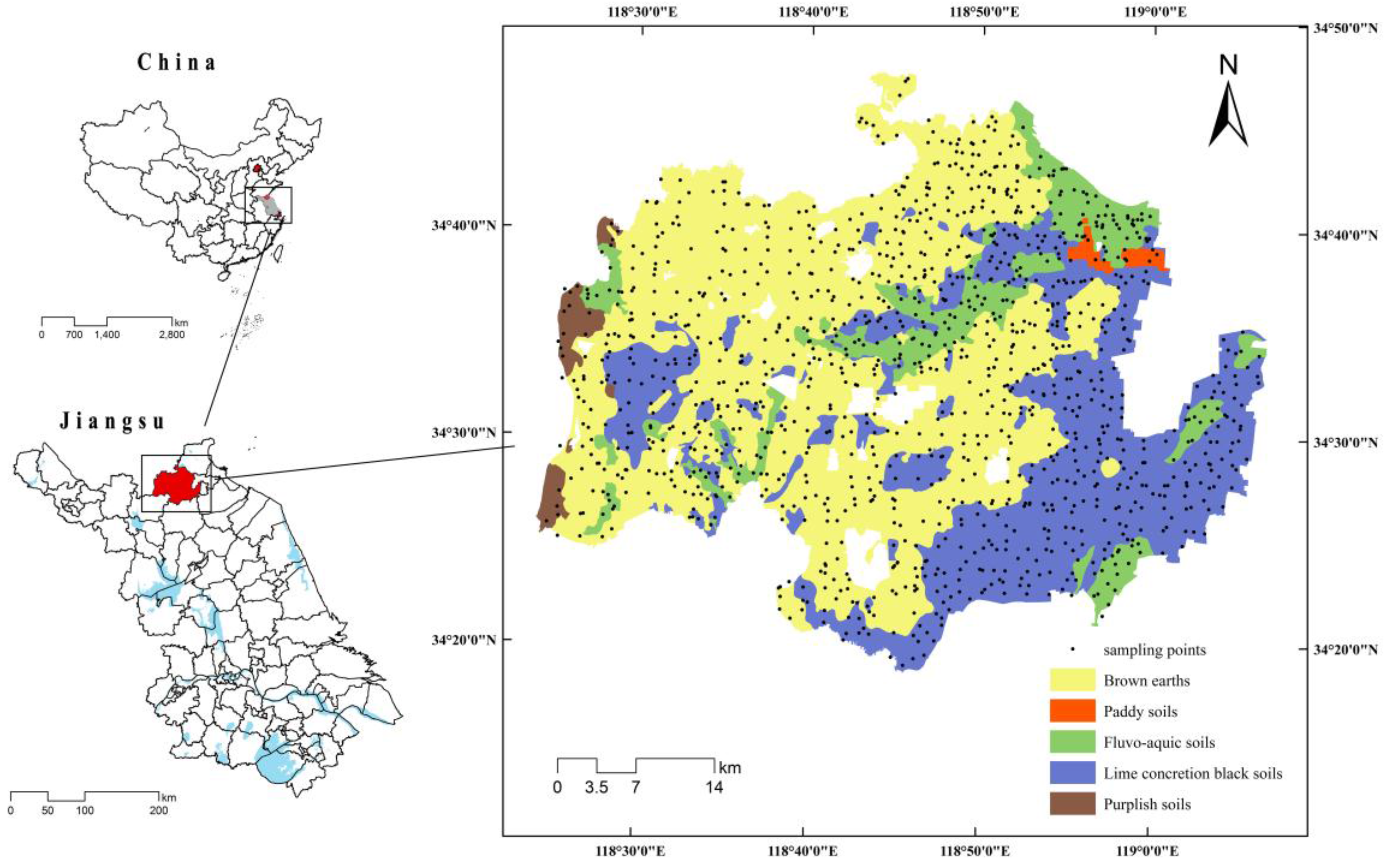
2.1.1. Study Area
2.1.2. Soil Sample Points
2.2. Methods
2.2.1. Spatial Variation Analysis
2.2.2. Spatial Variation-Based Simulated Annealing (SA) Algorithm
2.2.3. Statistical Analysis
3. Results
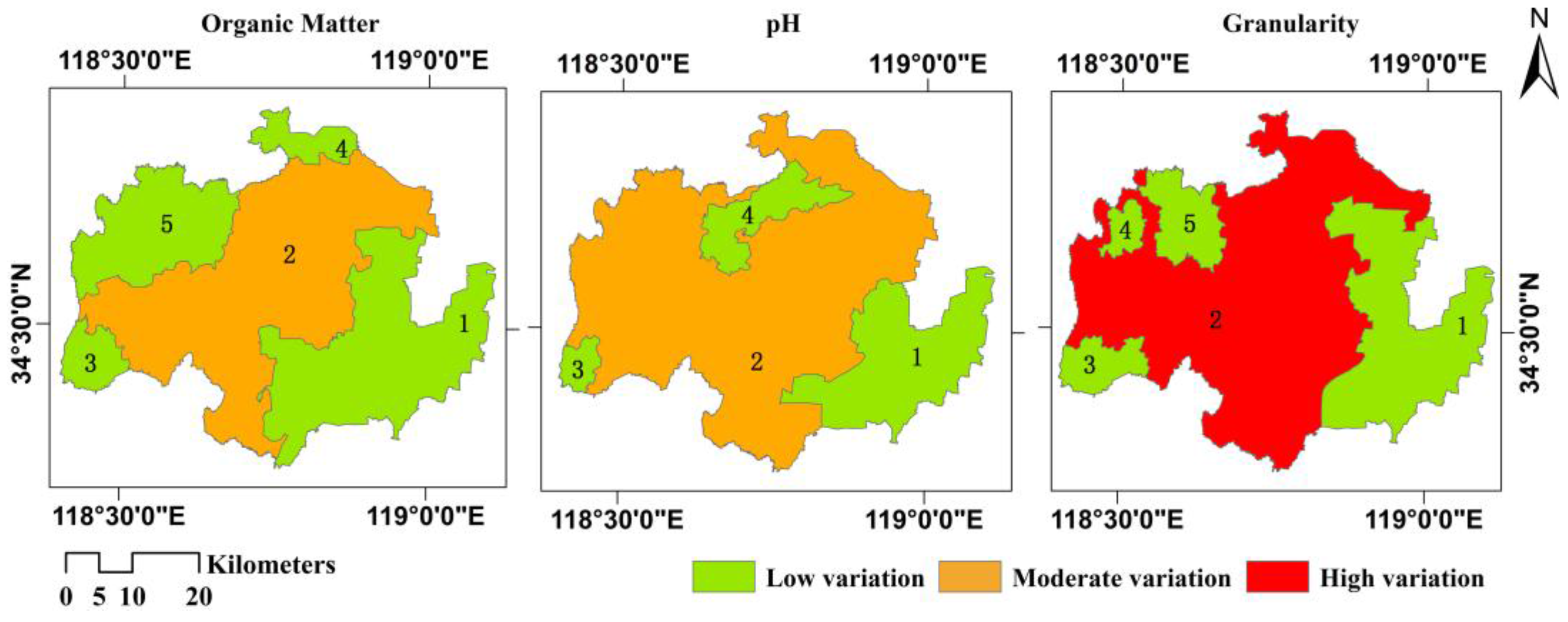
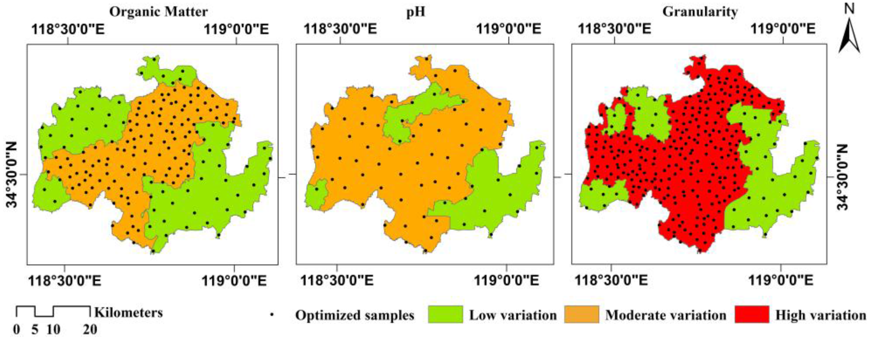
3.1. Spatial Variation Partitions
3.2. Conventional and Improved Simulated Annealing (SA)
4. Discussion
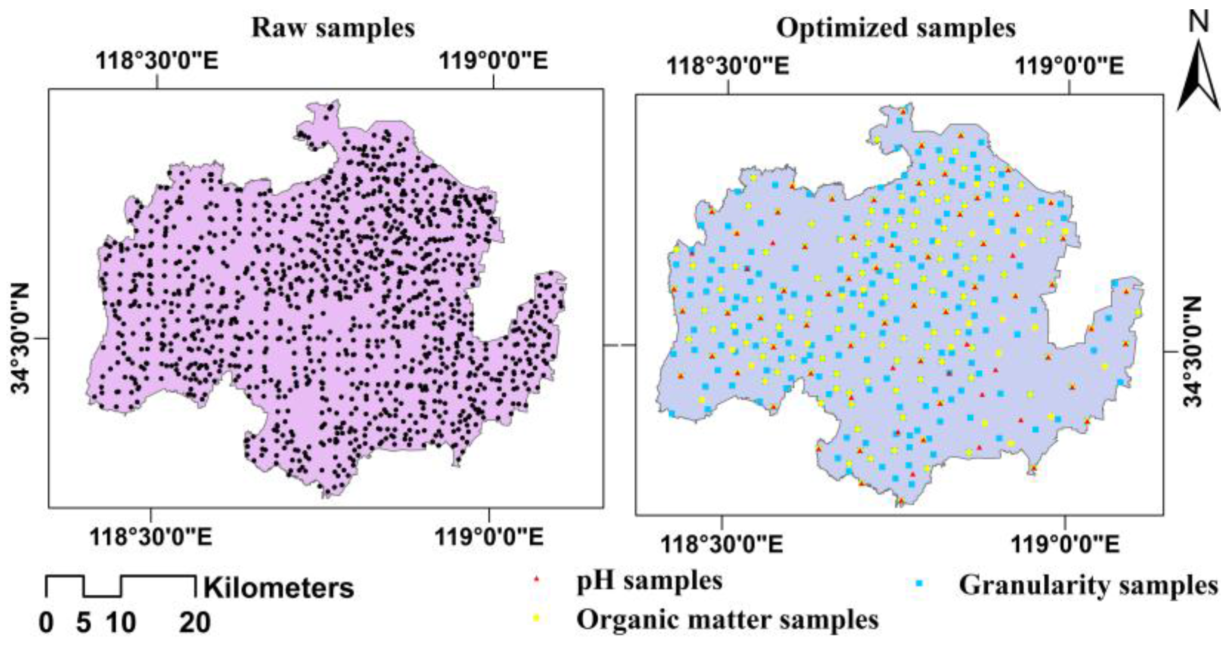
4.1. Comparison of Optimal and Raw Soil Sample Points
4.2. Prediction Accuracy of Arable Land Quality Based on Optimal Soil Sample Points
4.3. Analysis of Optimal Sample Points
5. Conclusions
Acknowledgments
Author Contributions
Conflicts of Interest
References
- Brown, G.P. Arable land loss in rural China: Policy and implementation in Jiangsu Province. Asian Surv. 1995, 35, 922–940. [Google Scholar] [CrossRef]
- Papadopoulou-Vrynioti, K.; Alexakis, D.; Bathrellos, G.D.; Skilodimou, H.D.; Vryniotis, D.; Vassiliades, E. Environmental research and evaluation of agricultural soil of the Arta plain, western Hellas. J. Geochem. Explor. 2014, 136, 84–92. [Google Scholar] [CrossRef]
- Zhao, Q.-G.; Zhou, B.-Z.; Yang, H.; Liu, S.-L. Chinese cultivated land resources, security issues and related countermeasures. Soil 2002, 34, 293–302. (In Chinese) [Google Scholar]
- Li, C.S.; Zhuang, Y.H.; Cao, M.Q.; Crill, P.; Dai, Z.H.; Frolking, S.; Moore, B., III; Salas, W.; Song, W.Z.; Wang, X.K. Comparing a process-based agro-ecosystem model to the IPCC methodology for developing a national inventory of N2O emissions from arable lands in China. Nutr. Cycl. Agroecosyst. 2001, 60, 159–175. [Google Scholar] [CrossRef]
- Sun, C.; Liu, G.; Xue, S. Land-use conversion changes the multifractal features of particle-size distribution on the Loess Plateau of China. Int. J. Environ. Res. Public Health 2016, 13, 785. [Google Scholar] [CrossRef] [PubMed]
- Liu, Y.S.; Wang, J.Y.; Long, H.L. Analysis of arable land loss and its impact on rural sustainability in southern Jiangsu Province of China. J. Environ. Manag. 2010, 91, 646–653. [Google Scholar] [CrossRef] [PubMed]
- Guedes, L.P.C.; Uribe-Opazo, M.A.; Ribeiro Junior, P.J. Optimization of sample design sizes and shapes for regionalized variables using simulated annealing. Ciencia Investig. Agraria 2014, 41, 33–48. [Google Scholar] [CrossRef]
- Amador, J.A.; Wang, Y.; Savin, M.C.; Görres, J.H. Fine-scale spatial variability of physical and biological soil properties in Kingston, Rhode Island. Geoderma 2000, 98, 83–94. [Google Scholar] [CrossRef]
- González-Peñaloza, F.A.; Cerdà, A.; Zavala, L.M.; Jordán, A.; Giménez-Morera, A.; Arcenegui, V. Do conservative agriculture practices increase soil water repellency? A case study in citrus-cropped soils. Soil Tillage Res. 2012, 124, 233–239. [Google Scholar] [CrossRef]
- Buttafuoco, G.; Tarvainen, T.; Jarva, J.; Guagliardi, I. Spatial variability and trigger values of arsenic in the surface urban soils of the cities of Tampere and Lahti, Finland. Environ. Earth Sci. 2016, 75, 896. [Google Scholar] [CrossRef]
- Qiu, J.; Wang, L.; Tang, H.; Li, H.; Li, C. Study on the situation of soil organic carbon storage in arable lands in Northeast China. Sci. Agric. Sin. 2004, 37, 1166–1171. (In Chinese) [Google Scholar]
- Papadopoulou-Vrynioti, K.; Alexakis, D.; Bathrellos, G.D.; Skilodimou, H.D.; Vryniotis, D.; Vassiliades, E.; Gamvroula, D. Distribution of trace elements in stream sediments of Arta plain (western Hellas): The influence of geomorphological parameters. J. Geochem. Explor. 2013, 134, 17–26. [Google Scholar] [CrossRef]
- Gessler, P.E.; Chadwick, O.A.; Chamran, F.; Althouse, L.; Holmes, K. Modeling soil—Landscape and ecosystem properties using terrain attributes. Soil Sci. Soc. Am. J. 2000, 64, 2046–2056. [Google Scholar] [CrossRef]
- Gessler, P.E.; Moore, I.D.; McKenzie, N.J.; Ryan, P.J. Soil-landscape modelling and spatial prediction of soil attributes. Int. J. Geogr. Inf. Sci. 1995, 9, 421–432. [Google Scholar] [CrossRef]
- Tan, M.; Li, X.; Xie, H.; Lu, C. Urban land expansion and arable land loss in China—A case study of Beijing-Tianjin-Hebei region. Land Use Policy 2005, 22, 187–196. [Google Scholar] [CrossRef]
- Bishop, T.F.A.; McBratney, A.B.; Whelan, B.M. Measuring the quality of digital soil maps using information criteria. Geoderma 2001, 103, 95–111. [Google Scholar] [CrossRef]
- Basile, A.; Buttafuoco, G.; Mele, G.; Tedeschi, A. Complementary techniques to assess physical properties of a fine soil irrigated with saline water. Environ. Earth Sci. 2012, 66, 1797–1807. [Google Scholar] [CrossRef]
- Brooks, S.P.; Morgan, B.J.T. Optimization using simulated annealing. Statistician 1995, 44, 241–257. [Google Scholar] [CrossRef]
- Ferreyra, R.A.; Apezteguı́a, H.P.; Sereno, R.; Jones, J.W. Reduction of soil water spatial sampling density using scaled semivariograms and simulated annealing. Geoderma 2002, 110, 265–289. [Google Scholar] [CrossRef]
- Simbahan, G.C.; Dobermann, A. Sampling optimization based on secondary information and its utilization in soil carbon mapping. Geoderma 2006, 133, 345–362. [Google Scholar] [CrossRef]
- Brown, P.D.; Cochrane, T.A.; Krom, T.D. Optimal on-farm irrigation scheduling with a seasonal water limit using simulated annealing. Agric. Water Manag. 2010, 97, 892–900. [Google Scholar] [CrossRef]
- Lark, R.M.; Papritz, A. Fitting a linear model of coregionalization for soil properties using simulated annealing. Geoderma 2003, 115, 245–260. [Google Scholar] [CrossRef]
- Chen, Y.-J.; Xiao, B.-L.; Fang, L.-N.; Ma, H.-L.; Yang, R.-Z.; Yi, X.-Y.; Li, Q.-Q. The quality analysis of cultivated land in China. Sci. Agric. Sin. 2011, 44, 3557–3564. (In Chinese) [Google Scholar]
- Xia, J.-G.; Li, T.-X.; Deng, L.-J.; Wu, X.; Wei, G.-H. The application of the principal component analysis method in quality evaluation of cultivated land. Southwest China J. Agric. Sci. 2000, 13, 51–55. (In Chinese) [Google Scholar]
- Xie, Y.; Mei, Y.; Guangjin, T.; Xuerong, X. Socio-economic driving forces of arable land conversion: A case study of Wuxian City, China. Glob. Environ. Chang. 2005, 15, 238–252. [Google Scholar] [CrossRef]
- Liu, Y.-S.; Wang, J.-Y.; Guo, L.-Y. The spatial-temporal changes of grain production and arable land in China. Sci. Agric. Sin. 2009, 42, 4269–4274. (In Chinese) [Google Scholar]
- Sun, L.; Chen, Y.; Lynn, H.; Wang, Q.; Zhang, S.; Li, R.; Xia, C.; Jiang, Q.; Hu, Y.; Gao, F.; et al. Identifying spatial Clusters of schistosomiasis in Anhui Province of China: A study from the perspective of application. Int. J. Environ. Res. Public Health 2015, 12, 11756–11769. [Google Scholar] [CrossRef] [PubMed]
- Huo, X.-N.; Li, H.; Sun, D.-F.; Zhou, L.-D.; Li, B.-G. Combining geostatistics with Moran’s I analysis for mapping soil heavy metals in Beijing, China. Int. J. Environ. Res. Public Health 2012, 9, 995–1017. [Google Scholar] [CrossRef] [PubMed]
- Chimi-Chiadjeu, O.; Vannier, E.; Dusséaux, R.; Le Hégarat-Mascle, S.; Taconet, O. Using simulated annealing algorithm to move clod boundaries on seedbed digital elevation model. Comput. Geosci. 2013, 57, 68–76. [Google Scholar] [CrossRef]
- Nunes, L.M.; Caeiro, S.; Cunha, M.C.; Ribeiro, L. Optimal estuarine sediment monitoring network design with simulated annealing. J. Environ. Manag. 2006, 78, 294–304. [Google Scholar] [CrossRef] [PubMed]
- Xia, Y.; Liu, D.; Liu, Y.; He, J.; Hong, X. Alternative zoning scenarios for regional sustainable land use controls in China: A knowledge-based multiobjective optimisation model. Int. J. Environ. Res. Public Health 2014, 11, 8839–8866. [Google Scholar] [CrossRef] [PubMed]


| Conventional Simulated Annealing | ||||||
| Indicator | Number of Optimal Sample Points | Percentage of Optimal Sample Points | Range of Effective Sample Points | Proportion of Effective Sample Points | RMSE | ANOVA |
| Organic matter | 226 | 17.38% | 57–1245 | 4.38%–95.77% | 0.49 | ** |
| pH | 78 | 6.00% | 35–1266 | 2.69%–97.38% | 0.44 | * |
| Granularity | 418 | 32.15% | 103–1274 | 7.92%–98.00% | 15.54 | ** |
| Improved Simulated Annealing | ||||||
| Indicator | Number of Optimal Sample Points | Percentage of Optimal Sample Points | Range of Effective Sample Points | Proportion of Effective Sample Points | RMSE | ANOVA |
| Organic matter | 178 | 13.69% | 52–1251 | 4.00%–96.23% | 0.50 | ** |
| pH | 72 | 5.54% | 31–1273 | 2.38%–97.92% | 0.44 | * |
| Granularity | 315 | 24.23% | 88–1280 | 6.77%–98.46% | 15.57 | ** |
| Parameter | Organic Matter (g/kg) | pH | Granularity (%) | |||
|---|---|---|---|---|---|---|
| Raw Sample Points (n = 1300) | Optimal Sample Points (n = 178) | Raw Sample Points (n = 1300) | Optimal Sample Points (n = 72) | Raw Sample Points (n = 1300) | Optimal Sample Points (n = 315) | |
| Minimum | 1.2 | 6.6 | 5.0 | 5.0 | 3.5 | 3.5 |
| Maximum | 41.0 | 37.0 | 9.9 | 8.9 | 89.7 | 88.6 |
| Mean | 18.4 | 17.6 | 6.7 | 6.7 | 34.1 | 30.9 |
| Skewness | 0.51 | 0.8 | 0.35 | 0.96 | 0.61 | 1.26 |
| Kurtosis | –0.3 | 0.38 | 0.77 | 1.16 | −0.96 | 0.61 |
| Coefficient of variation | 37.33% | 37.28% | 8.64% | 6.00% | 69.32% | 72.28% |
| ANOVA | ** | * | ** | |||
| Soil Property | Spatial Variation | ||
|---|---|---|---|
| Raw Sample Points | Optimal Sample Points from Conventional SA | Optimal Sample Points from Improved SA | |
| Organic matter | 0.3458 | 0.3412 | 0.4288 |
| pH | 0.4700 | 0.4553 | 0.4859 |
| Granularity | 0.4898 | 0.5001 | 0.6423 |
| Soil Property | Low-Variation Partitions | Moderate- and High-Variation Partitions | ||||
|---|---|---|---|---|---|---|
| Raw Sample Points | Optimal Sample Points | Percentage of Optimal Sample Points | Raw Sample Points | Optimal Sample Points | Percentage of Optimal Sample Points | |
| Organic matter | 631 | 58 | 9.19% | 669 | 120 | 17.94% |
| pH | 388 | 19 | 4.90% | 912 | 53 | 5.81% |
| Granularity | 486 | 46 | 9.47% | 814 | 269 | 33.05% |
| Soil Property | Raw Sample Points | Optimal Sample Points from Conventional SA | Optimal Sample Points from Improved SA | |||
|---|---|---|---|---|---|---|
| Number | Prediction Accuracy (R2) | Number | Prediction Accuracy (R2) | Number | Prediction Accuracy (R2) | |
| Organic matter | 1300 | 0.8823 | 226 | 0.8331 | 178 | 0.8926 |
| pH | 1300 | 0.7363 | 78 | 0.7108 | 72 | 0.7488 |
| Granularity | 1300 | 0.8527 | 418 | 0.8116 | 315 | 0.8693 |
| Source | Number | Percentage |
|---|---|---|
| Optimal sample points for organic matter only | 25 | 7.16% |
| Optimal sample points for pH only | 12 | 3.44% |
| Optimal sample points for granularity only | 158 | 45.27% |
| Optimal sample points for organic matter and pH | 12 | 3.44% |
| Optimal sample points for organic matter and granularity | 94 | 26.93% |
| Optimal sample points for pH and granularity | 2 | 0.57% |
| Optimal sample points for organic matter, pH, and granularity | 46 | 13.18% |
© 2016 by the authors; licensee MDPI, Basel, Switzerland. This article is an open access article distributed under the terms and conditions of the Creative Commons Attribution (CC-BY) license (http://creativecommons.org/licenses/by/4.0/).
Share and Cite
Wang, J.; Wang, X.; Zhou, S.; Wu, S.; Zhu, Y.; Lu, C. Optimization of Sample Points for Monitoring Arable Land Quality by Simulated Annealing while Considering Spatial Variations. Int. J. Environ. Res. Public Health 2016, 13, 980. https://doi.org/10.3390/ijerph13100980
Wang J, Wang X, Zhou S, Wu S, Zhu Y, Lu C. Optimization of Sample Points for Monitoring Arable Land Quality by Simulated Annealing while Considering Spatial Variations. International Journal of Environmental Research and Public Health. 2016; 13(10):980. https://doi.org/10.3390/ijerph13100980
Chicago/Turabian StyleWang, Junxiao, Xiaorui Wang, Shenglu Zhou, Shaohua Wu, Yan Zhu, and Chunfeng Lu. 2016. "Optimization of Sample Points for Monitoring Arable Land Quality by Simulated Annealing while Considering Spatial Variations" International Journal of Environmental Research and Public Health 13, no. 10: 980. https://doi.org/10.3390/ijerph13100980
APA StyleWang, J., Wang, X., Zhou, S., Wu, S., Zhu, Y., & Lu, C. (2016). Optimization of Sample Points for Monitoring Arable Land Quality by Simulated Annealing while Considering Spatial Variations. International Journal of Environmental Research and Public Health, 13(10), 980. https://doi.org/10.3390/ijerph13100980