
Model Averaging for Improving Inference from Causal Diagrams

Abstract
:1. Introduction
1.1. Uncertainty in Causal Modeling
1.2. Averaging Models to Avoid Investigator Bias
2. Methods
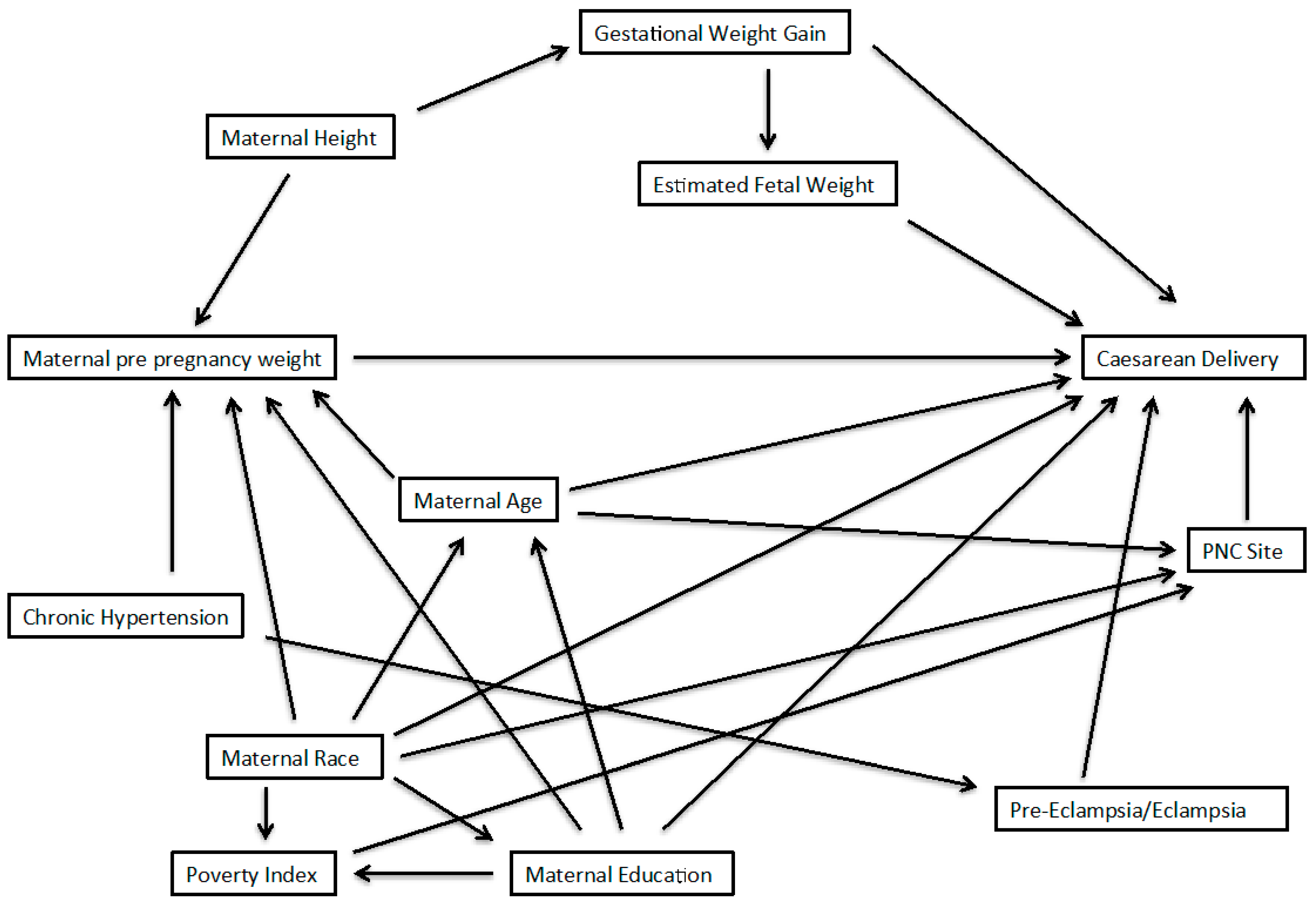
2.1. Example from the PIN Study
2.2. Three Approaches for Model Averaging
3. Results

| Adjustment Set | Covariates | Overweight vs. Normal | Obese vs. Normal | ||||
|---|---|---|---|---|---|---|---|
| Risk Ratio | 95% CI | Risk Ratio | 95% CI | AIC | Weight | ||
| 1 | Chronic hypertension, gestational weight gain, maternal age, maternal education, maternal race | 1.38 | 0.92, 2.09 | 1.75 | 1.23, 2.50 | 552.56 | 0.43 |
| 2 | Chronic hypertension, maternal age, maternal education, maternal race, maternal height | 1.27 | 0.84, 1.92 | 1.46 | 1.04, 2.08 | 552.74 | 0.39 |
| 3 | Gestational weight gain, maternal age, maternal education, maternal race, pre-eclampsia/eclampsia | 1.38 | 0.91, 2.09 | 1.74 | 1.22, 2.48 | 555.12 | 0.12 |
| 4 | Maternal age, maternal education, maternal height, maternal race, pre-eclampsia/eclampsia | 1.29 | 0.85, 1.95 | 1.48 | 1.05, 2.10 | 556.43 | 0.06 |
| AIC Averaged values | 1.33 | 0.86, 2.03 | 1.62 | 1.09, 2.39 | |||
| Overweight vs. Normal | Obese vs. Normal | |||
|---|---|---|---|---|
| Adjustment Set | Risk Ratio | 95% CI | Risk Ratio | 95% CI |
| 1 | 1.41 | 0.93, 2.11 | 1.86 | 1.32, 2.62 |
| 2 | 1.35 | 0.92, 2.00 | 1.48 | 1.06, 2.06 |
| 3 | 1.38 | 0.91, 2.09 | 1.74 | 1.22, 2.48 |
| 4 | 1.33 | 0.89, 1.97 | 1.43 | 1.02, 2.01 |
| Average | 1.37 | 0.92, 2.04 | 1.61 | 1.15, 2.27 |
| Overweight vs. Normal | Obese vs. Normal | |||||
|---|---|---|---|---|---|---|
| Adjustment Set | Risk Ratio | 95% Interval † | Risk Ratio | 95% Interval † | ||
| Mean | Median | Mean | Median | |||
| 1 | 1.39 | 1.36 | 0.92, 2.02 | 1.78 | 1.76 | 1.28, 2.46 |
| 2 | 1.34 | 1.31 | 0.90, 1.93 | 1.45 | 1.42 | 1.07, 1.98 |
| 3 | 1.40 | 1.38 | 0.87, 2.08 | 1.76 | 1.73 | 1.18, 2.50 |
| 4 | 1.34 | 1.32 | 0.87, 1.96 | 1.43 | 1.41 | 1.01, 1.99 |
| Average | 1.37 | 1.34 | 0.89, 2.01 | 1.60 | 1.57 | 1.07, 2.35 |
| Averaging Approach | Overweight | Obese |
|---|---|---|
| Akaike’s Information | 2.36 | 2.19 |
| Inverse Variance | 2.22 | 1.97 |
| Bootstrap resampling | 2.26 | 2.20 |
4. Discussion
5. Conclusions
Supplementary Material
1. AIC Model Averaging
2. Inverse Variance Weighting
3. Software code for recreating model averaged results for bootstrap and AIC techniques
     SAS code
      *********************************************************************************
      ***** Model averaging via bootstrapping
      ***** hamrag@fellows.iarc.fr
      ***** Example from PIN study (UNC, Chapel Hill)
      ***** To request PIN data, please visit:
      ***** http://www.cpc.unc.edu/projects/pin/datause
      ********************************************************************************;
	  ** Import data;
      procimport out=one datafile='YOUR Directory'
      dbms=csv replace; getnames=yes; run;
	  ** Recode variables from data so there are 0 references;
      data one;
            set one;
            bmi = C_BMIIOM - 2;
            medu = edu - 1;
            height = C_INCHES - 65.04; *Center height at mean;
            if ind = 0 then induction = 0;
                  else induction = 1;
            run;
        *********************************************
        ***** Bootstrap data, 1000 replications
        *********************************************;
        procsurveyselect data=one out=pinboot
            seed = 280420141
            method = urs
            samprate = 100
            outhits
            rep = 1000;
        run;
        *****************************************************************
        ***** Fit 4 minimally sufficient models, output data from each
        *****************************************************************;
        * Model 1: adjust: hypertension, gestational weight gain, maternal age/edu/race;
        ods output ParameterEstimates = m1out;
        procgenmod data=pinboot desc;
            by Replicate;
            class bmi(ref=first);
            model cesarean = bmi hyper C_WTGAIN mom_age medu race /dist=binomial link=log;
        run;
        * Model 2: adjust: hypertension, maternal age/edu/race/height;
        ods output ParameterEstimates = m2out;
        procgenmod data=pinboot desc;
            by Replicate;
            class bmi(ref=first);
            model cesarean = bmi hyper mom_age medu race height/dist=binomial link=log;
        run;
        * Model 3: adjust: gestational weight gain, maternal age/edu/race, eclampsia;
        ods output ParameterEstimates = m3out;
        procgenmod data=pinboot desc;
            by Replicate;
            class bmi(ref=first);
            model cesarean = bmi C_WTGAIN mom_age medu race eclamp/dist=binomial link=log;
        run;
        * Model 4: adjust: maternal age/edu/race/height, eclampsia;
        ods output ParameterEstimates = m4out;
        procgenmod data=pinboot desc;
            by Replicate;
            class bmi(ref=first);
            model cesarean = bmi mom_age medu race height eclamp/dist=binomial link=log;
        run;
        **********************************************
        ****Extract BMI values from each dataset
        ****First, for overweight vs normal
        **********************************************;
        data m1over (keep = Estimate Replicate model);
            set m1out;
            if Parameter = 'bmi' AND Level1 = 1;
            model = 1;
            run;
        data m2over (keep = Estimate Replicate model);
            set m2out;
            if Parameter = 'bmi' AND Level1 = 1;
            model = 2;
            run;
        data m3over (keep = Estimate Replicate model);
            set m3out;
            if Parameter = 'bmi' AND Level1 = 1;
            model = 3;
            run;
        data m4over (keep = Estimate Replicate model);
            set m4out;
            if Parameter = 'bmi' AND Level1 = 1;
            model = 4;
            run;
        **** Pool datasets and summarize estimate;
        data over;
            set m1over m2over m3over m4over;
            exp = exp(Estimate);
            run;
        *summary of bootstrap estimates by adjustment set;
        procunivariate data=over;
            by model;
            var exp;
            output out= over1a mean=mean pctlpts = 2.5, 50, 97.5 pctlpre=ci;
        run;
        *Model average of overweight versus normal weight;
        procunivariate data=over;
            var exp;
            output out= over1b mean=mean pctlpts = 2.5, 50, 97.5 pctlpre=ci;
        run;
        **********************************************
        ** Repeat above for obese versus normal
        *********************************************;
        data m1obese (keep = Estimate Replicate model);
            set m1out;
            if Parameter = 'bmi' AND Level1 = 2;
            model = 1;
            run;
        data m2obese (keep = Estimate Replicate model);
            set m2out;
            if Parameter = 'bmi' AND Level1 = 2;
            model = 2;
            run;
        data m3obese (keep = Estimate Replicate model);
            set m3out;
            if Parameter = 'bmi' AND Level1 = 2;
            model = 3;
            run;
        data m4obese (keep = Estimate Replicate model);
            set m4out;
            if Parameter = 'bmi' AND Level1 = 2;
            model = 4;
            run;
        **** Pool datasets and summarize estimate;
        data obese;
            set m1obese m2obese m3obese m4obese;
            exp = exp(Estimate);
            run;
        *summary of bootstrap estimates by adjustment set;
        procunivariate data=obese;
            by model;
            var exp;
            output out= obese1a mean=mean pctlpts = 2.5, 50, 97.5 pctlpre=ci;
        run;
        *Model average of overweight versus normal weight;
        procunivariate data=obese;
            var exp;
            output out= obese1b mean=mean pctlpts = 2.5, 50, 97.5 pctlpre=ci;
        run;
        *end of file;
        R code
        ###########################################################################
        ##### Multi-model inference with AIC weighting
        ###########################################################################
        ## Load relevant libraries and set working directory
        library(Epi)
        library(foreign)
        library(MuMIn)
        library(boot)
        setwd('Your directory')
        ## load and summarize data
        PIN <- read.csv('PIN.csv',header=T)
        str(PIN)
        ## Re-code BMI and Education so there is a zero referent
        ## also center height and record induction
        PIN$BMI <- PIN$C_BMIIOM - 2
        PIN$m_edu <- PIN$edu - 1
        PIN$height <- PIN$C_INCHES - 65.04 # center height
        PIN$induction <- as.numeric(ifelse(PIN$ind==0,0,1)) # categorize induction into 0,1
        ####################################################
        ## Average over all minimally sufficient adjustment sets
        ####################################################
        ## restrict data to exclude missings. Necessary for averaging with AIC!
        keep <- c('cesarean','BMI','hyper','C_WTGAIN','mom_age','m_edu',
         'race','height','eclamp')
        PIN1 <- na.omit(PIN[keep])
        attach(PIN1)
        #################################################################
        ## NOTE: some models run with reduced adjustment sets to obtain
        ## starting values that help with model convergence
        #################################################################
        ## model 1: hypertension, gestational weight gain, maternal age/edu/race
        m1a <- glm(cesarean ~ factor(BMI) + hyper + C_WTGAIN +
         mom_age + m_edu + race,
         family=binomial(link='log'))
        m1 <- glm(cesarean ~ factor(BMI) + hyper + C_WTGAIN +
         mom_age + m_edu + race,
         family=binomial(link='log'))
        summary(m1)
        ci.exp(m1)
        ## model 2: hypertension, maternal age/edu/race/height
        m2a <- glm(cesarean ~ factor(BMI) + hyper + mom_age + m_edu +
         race,
         family=binomial(link='log'))
        m2 <- glm(cesarean ~ factor(BMI) + hyper + mom_age + m_edu +
         race + height,
         family=binomial(link='log'), start=c(coef(m2a),0))
        summary(m2)
        ci.exp(m2)
        ## model 3: gestational weight gain, maternal age/edu/race, eclampsia
        m3 <- glm(cesarean ~ factor(BMI) + C_WTGAIN + mom_age + m_edu +
         race + eclamp,
         family=binomial(link='log'))
        summary(m3)
        ci.exp(m3)
        ## model 4: maternal age/edu/race/height, eclampsia
        m4a <- glm(cesarean ~ factor(BMI) + mom_age + m_edu + race +
         eclamp,
         family=binomial(link='log'))
        m4 <- glm(cesarean ~ factor(BMI) + mom_age + m_edu + race +
         eclamp + height,
         family=binomial(link='log'), start=c(coef(m4a),0))
        summary(m4)
        ci.exp(m4)
        ## Average the results of the four models above
        models <- list(m1,m2,m3,m4)
        AIC_avg <- model.avg(models, rank=AIC, cumsum(weight)<=0.95)
        summary(AIC_avg)
        confint(AIC_avg)
        #end of file
Acknowledgments
Author Contributions
Conflicts of Interest
References
- Robins, J.M.; Greenland, S. The role of model selection in causal inference from nonexperimental data. Am. J. Epidemiol. 1986, 123, 392–402. [Google Scholar] [PubMed]
- Wynder, E.L.; Higgins, I.T.; Harris, R.E. The wish bias. J. Clin. Epidemiol. 1990, 43, 619–621. [Google Scholar] [PubMed]
- Cope, M.B.; Allison, D.B. White hat bias: Examples of its presence in obesity research and a call for renewed commitment to faithfulness in research reporting. Int. J. Obes. 2010, 34, 84–88. [Google Scholar]
- Cope, M.B.; Allison, D.B. White hat bias: A threat to the integrity of scientific reporting. Acta Paediatr. 2010, 99, 1615–1617. [Google Scholar] [PubMed]
- Greenland, S.; Pearl, J.; Robins, J.M. Causal diagrams for epidemiologic research. Epidemiology 1999, 10, 37–48. [Google Scholar] [CrossRef] [PubMed]
- Pearl, J. Causality: Models, Reasoning, and Inference; Cambridge University Press: New York, NY, USA, 2000. [Google Scholar]
- Raftery, A.E. Bayesian model selection in social research. Sociol. Methodol. 1995, 25, 111–163. [Google Scholar] [CrossRef]
- Viallefont, V.; Raftery, A.E.; Richardson, S. Variable selection and Bayesian model averaging in case-control studies. Stat. Med. 2001, 20, 3215–3230. [Google Scholar] [CrossRef] [PubMed]
- Burnham, K.P.; Anderson, D.R. Model Selection and Multimodel Inference: A Practical Information-theoretic Approach, 2nd ed.; Springer: New York, NY, USA, 2002. [Google Scholar]
- VanderWeele, T.J.; Robins, J.M. Four types of effect modification: A classification based on directed acyclic graphs. Epidemiology 2007, 18, 561–568. [Google Scholar] [CrossRef] [PubMed]
- Shrier, I.; Platt, R.W. Reducing bias through directed acyclic graphs. BMC Med. Res. Methodol. 2008, 8, 70. [Google Scholar] [CrossRef] [PubMed]
- Lash, T.L.; Fox, M.P.; MacLehose, R.F.; Maldonado, G.; McCandless, L.C.; Greenland, S. Good practices for quantitative bias analysis. Int. J. Epidemiol. 2014, 43, 1969–1985. [Google Scholar] [CrossRef] [PubMed]
- Schisterman, E.F.; Cole, S.R.; Platt, R.W. Overadjustment bias and unnecessary adjustment in epidemiologic studies. Epidemiology 2009, 20, 488–495. [Google Scholar] [CrossRef] [PubMed]
- Naimi, A.I.; Cole, S.R.; Westreich, D.J.; Richardson, D.B. A comparison of methods to estimate the hazard ratio under conditions of time-varying confounding and nonpositivity. Epidemiology 2011, 22, 718–723. [Google Scholar] [CrossRef] [PubMed]
- Cole, S.R.; Frangakis, C.E. The consistency statement in causal inference: A definition or an assumption? Epidemiology 2009, 20, 3–5. [Google Scholar] [CrossRef]
- Sobel, M.E. What do randomized studies of housing mobility demonstrate? Causal inference in the face of interference. J. Am. Stat. Assoc. 2006, 101, 1398–1407. [Google Scholar] [CrossRef]
- Greenland, S. Randomization, statistics, and causal inference. Epidemiology 1990, 1, 421–429. [Google Scholar] [CrossRef] [PubMed]
- Cole, S.R.; Platt, R.W.; Schisterman, E.F.; Chu, H.; Westreich, D.; Richardson, D.; Poole, C. Illustrating bias due to conditioning on a collider. Int. J. Epidemiol. 2010, 39, 417–420. [Google Scholar] [CrossRef] [PubMed]
- Savitz, D.A.; Dole, N.; Williams, J.; Thorp, J.M.; McDonald, T.; Carter, A.C.; Eucker, B. Determinants of participation in an epidemiological study of preterm delivery. Paediatr. Perinat. Epidemiol. 1999, 13, 114–125. [Google Scholar] [CrossRef] [PubMed]
- Vahratian, A.; Siega-Riz, A.M.; Savitz, D.A.; Zhang, J. Maternal pre-pregnancy overweight and obesity and the risk of cesarean delivery in nulliparous women. Ann. Epidemiol. 2005, 15, 467–474. [Google Scholar] [CrossRef] [PubMed]
- Buckland, S.T.; Burnham, K.P.; Augustin, N.H. Model selection: An integral part of inference. Biometrics 1997, 53, 603–618. [Google Scholar] [CrossRef]
- Hoeting, J.A.; Madigan, D.; Raftery, A.E.; Volinsky, C.T. Bayesian model averaging: A tutorial. Statist. Sci. 1999, 14, 382–401. [Google Scholar]
- Rothman, K.J.; Greenland, S.; Lash, T.L. Modern Epidemiology, 3rd ed.; Lippincott Williams & Wilkins: Philadelphia, PA, USA, 2008. [Google Scholar]
- Cochrane Collaboration. In Cochrane Handbook for Systematic Reviews of Interventions; Higgins, J.P.T.; Green, S. (Eds.) Wiley-Blackwell: Hoboken, NJ, USA, 2008.
- Efron, B.; Tibshirani, R. An Introduction to the Bootstrap; Chapman & Hall: New York, NY, USA; CRC Press: Boca Raton, FL, USA, 1993. [Google Scholar]
- Poole, C. Low P-values or narrow confidence intervals: Which are more durable? Epidemiology 2001, 12, 291–294. [Google Scholar] [CrossRef] [PubMed]
- Dominici, F.; Wang, C.; Crainiceanu, C.; Parmigiani, G. Model selection and health effect estimation in environmental epidemiology. Epidemiology 2008, 19, 558–560. [Google Scholar] [CrossRef] [PubMed]
- Richardson, D.B.; Cole, S.R. Model averaging in the analysis of leukemia mortality among Japanese A-bomb survivors. Radiat. Environ. Biophys. 2012, 51, 93–95. [Google Scholar] [CrossRef] [PubMed]
- Greenland, S. Invited commentary: Variable selection versus shrinkage in the control of multiple confounders. Am. J. Epidemiol. 2008, 167, 523–529. [Google Scholar] [CrossRef] [PubMed]
- Rubin, D.B. The design versus the analysis of observational studies for causal effects: Parallels with the design of randomized trials. Stat. Med. 2007, 26, 20–36. [Google Scholar] [CrossRef] [PubMed]
- Brookhart, M.A.; Schneeweiss, S.; Rothman, K.J.; Glynn, R.J.; Avorn, J.; Sturmer, T. Variable selection for propensity score models. Am. J. Epidemiol. 2006, 163, 1149–1156. [Google Scholar] [CrossRef] [PubMed]
- Greenland, S.; Robins, J.M.; Pearl, J. Confounding and collapsibility in causal inference. Stat. Sci. 1999, 14, 29–46. [Google Scholar]
© 2015 by the authors; licensee MDPI, Basel, Switzerland. This article is an open access article distributed under the terms and conditions of the Creative Commons Attribution license (http://creativecommons.org/licenses/by/4.0/).
Share and Cite
Hamra, G.B.; Kaufman, J.S.; Vahratian, A. Model Averaging for Improving Inference from Causal Diagrams. Int. J. Environ. Res. Public Health 2015, 12, 9391-9407. https://doi.org/10.3390/ijerph120809391
Hamra GB, Kaufman JS, Vahratian A. Model Averaging for Improving Inference from Causal Diagrams. International Journal of Environmental Research and Public Health. 2015; 12(8):9391-9407. https://doi.org/10.3390/ijerph120809391
Chicago/Turabian StyleHamra, Ghassan B., Jay S. Kaufman, and Anjel Vahratian. 2015. "Model Averaging for Improving Inference from Causal Diagrams" International Journal of Environmental Research and Public Health 12, no. 8: 9391-9407. https://doi.org/10.3390/ijerph120809391
APA StyleHamra, G. B., Kaufman, J. S., & Vahratian, A. (2015). Model Averaging for Improving Inference from Causal Diagrams. International Journal of Environmental Research and Public Health, 12(8), 9391-9407. https://doi.org/10.3390/ijerph120809391