
Modeling Flows and Concentrations of Nine Engineered Nanomaterials in the Danish Environment


Abstract
:1. Introduction
2. Experimental Section
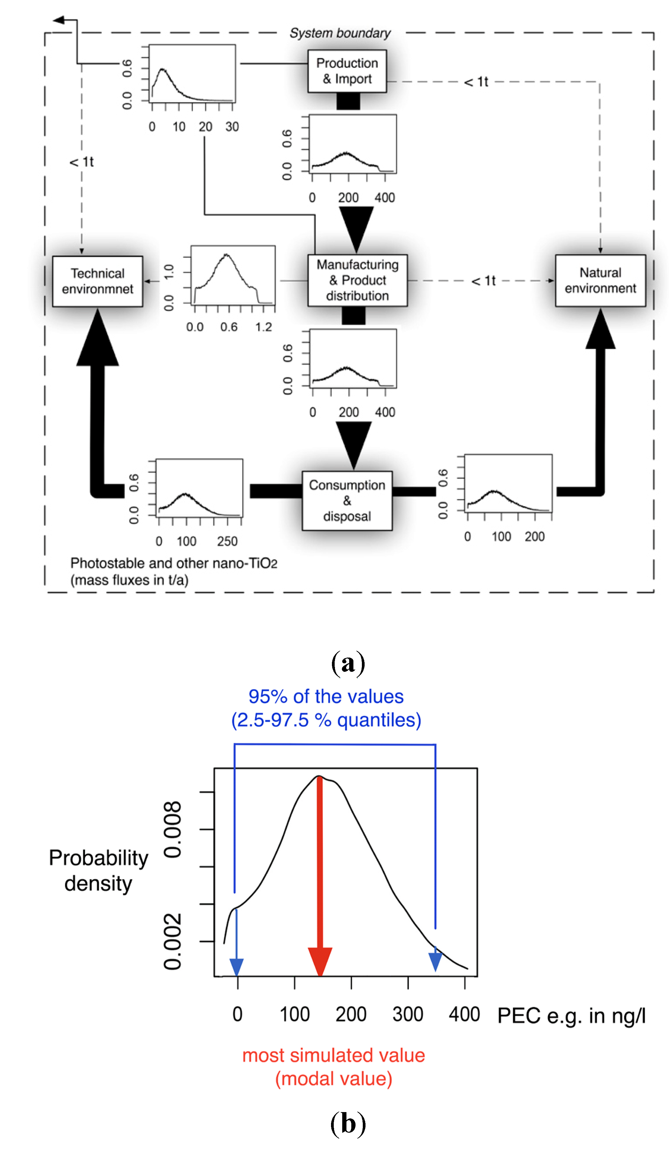
2.1. Environmental Exposure Model
2.2. The Probabilistic Flow Modeling
2.3. Nanomaterial Sources

| ENM | Main Uses | Used (t) |
|---|---|---|
| Photostable TiO2 | Plastics, cosmetics |  |
| Photocatalytic TiO2 | Paints, coating, construction materials, filters |  |
| ZnO | Cosmetics, paints |  |
| Ag | Textiles, paints, cleaning agents electronics, cosmetics |  |
| CuCO3 | Wood preservation |  |
| CNT | Polymer composites |  |
| CeO2 | Catalysts, fuel additive, polishing, paints |  |
| Quantum dots (QD) | LED, imaging |  |
| Carbon black (CB) | Tires, rubber, paints |  |
2.4. From Mass Flows to Predicted Environmental Concentrations
3. Results
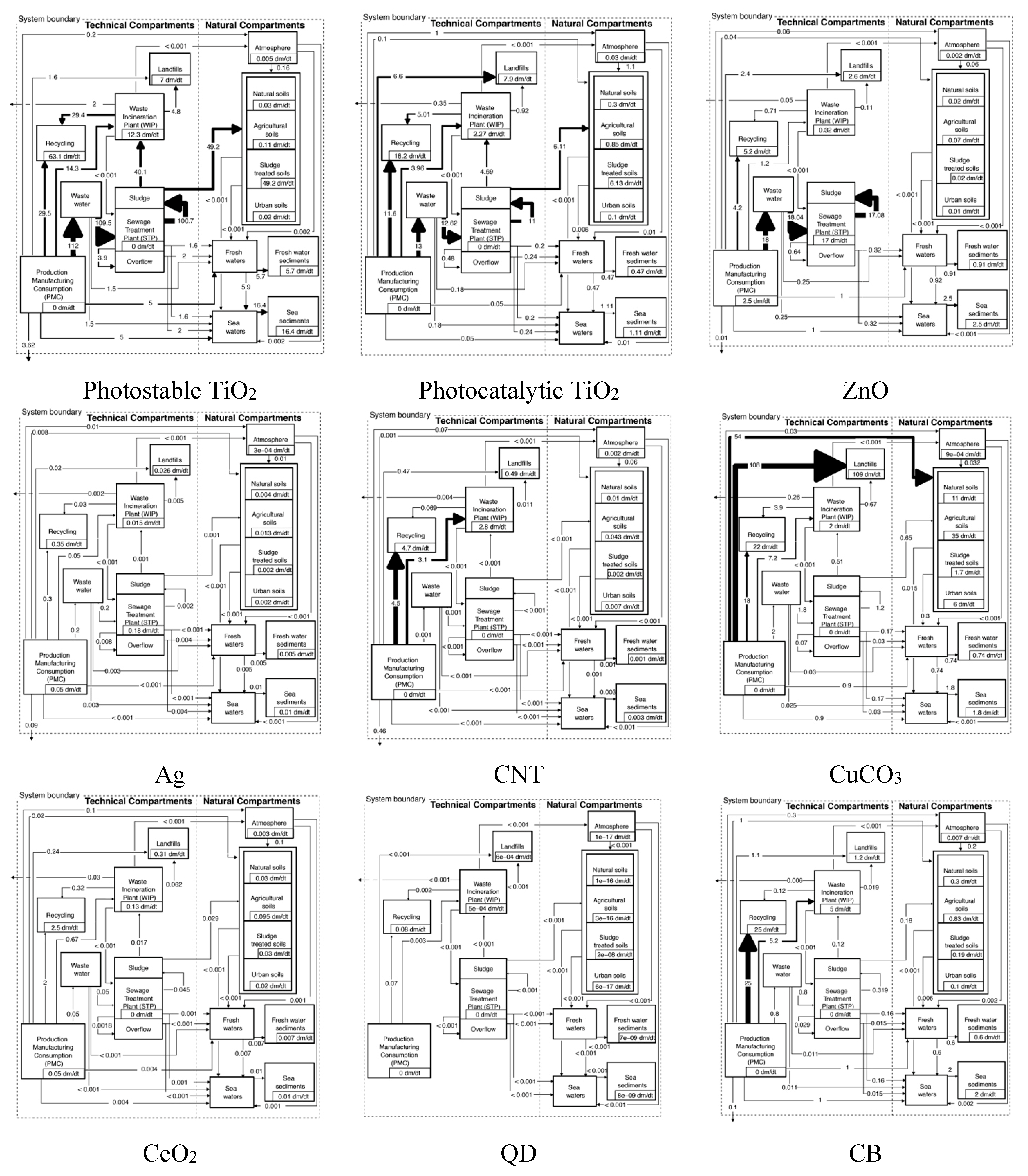
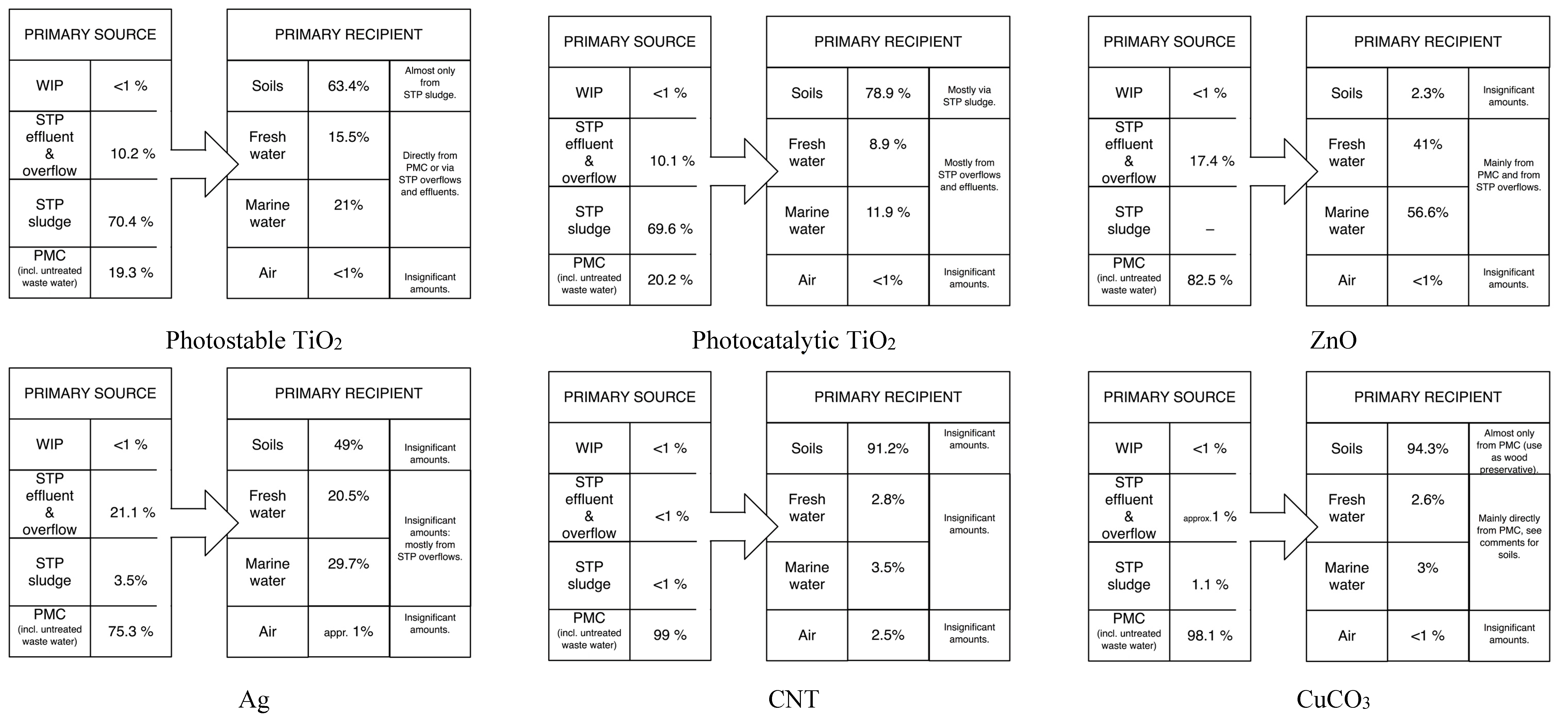
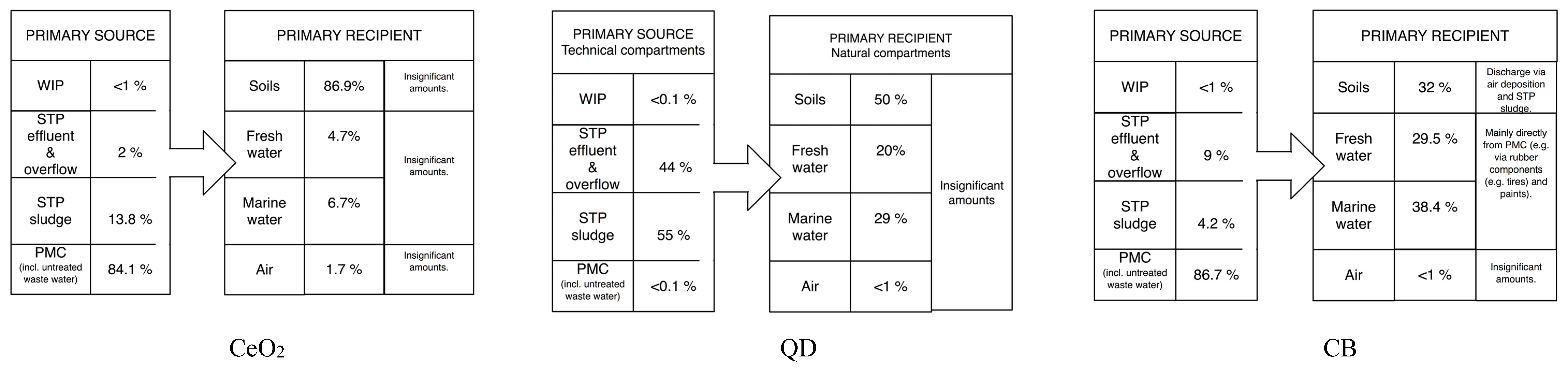
3.1. Material Flows
3.2. Concentrations in the Technical System


| Compartment | Unit | Photostable TiO2 | Photocatalytic TiO2 | ZnO | CuCO3 | ||||
|---|---|---|---|---|---|---|---|---|---|
| Mode | Range | Mode | Range | Mode | Range | Mode | Range | ||
| Technical compartments | |||||||||
| Sewage treatment effluent | µg/L | 13 | 3.4–92 | 1.6 | 0.4–14 | 0 | 1.3 | 0.3–4.1 | |
| Sewage treatment sludge | mg/kg | 770 | 69–1500 | 85 | 9.3–230 | 0 | 9.1 | 5.2–17 | |
| Waste mass incinerated | mg/kg | 15 | 1.4–32 | 2.8 | 0.3–6.8 | 0.3 | 0.04–1.5 | 2 | 1.3–3 |
| Bottom ash | mg/kg | 33 | 3.4–88 | 6 | 0.7–18 | 0.7 | 0.1–3.9 | 4.4 | 2.7–8.5 |
| Fly ash | mg/kg | 170 | 17–430 | 30 | 3.3–90 | 3.6 | 0.5–19 | 22 | 13–42 |
| Natural compartments | |||||||||
| Surface water (fresh water) | ng/L | 3 | 0.6–100 | 0.27 | 0.05–7 | 0.45 | 0.09–13 | 2 | 0.1–6 |
| Sea water | ng/L | 0.30 | 0.04–1 | 0.02 | 0.004–0.099 | 0.04 | 0.006–0.4 | 0.04 | 0.02–0.07 |
| Sediments (fresh water) | µg/kg | 1200 | 200–28,000 | 92 | 17–2600 | 160 | 30–4800 | 880 | 43–2100 |
| Sediments (sea water) | µg/kg | 390 | 49–1300 | 27 | 4.3–120 | 49 | 6–220 | 42 | 25–83 |
| Agricultural soils | µg/kg | 0.085 | 0.01–0.39 | 0.7 | 0.1–1.7 | 0.052 | 0.008–0.35 | 28 | 18–41 |
| Natural soils | µg/kg | 0.18 | 0.024–1.1 | 1.5 | 0.2–4.9 | 0.12 | 0.018–0.9 | 60 | 39–130 |
| Urban soils | µg/kg | 0.33 | 0.039–1.5 | 2.7 | 0.3–6.7 | 0.2 | 0.03–1.3 | 110 | 70–160 |
| Sludge treated soils | µg/kg | 1300 | 130–3100 | 170 | 17–480 | 0 | 0 | 48 | 32–70 |
| Air | ng/m3 | 0.10 | 0.01–0.5 | 0.70 | 0.08–2 | 0.04 | 0.005–0.2 | 0.02 | 0.005–0.04 |
| Unit | Ag | CNT | CeO2 | QD | |||||
| Mode | Range | Mode | Range | Mode | Range | Mode | Range | ||
| Technical compartments | |||||||||
| Sewage treatment effluent | ng/L | 0.5 | 0.012–59 | 0.3 | 0.1–3.5 | 9.3 | 1.1–60 | 3.00E−05 | 5E−6–0.001 |
| Sewage treatment sludge | µg/kg | 82 | 4.2–250 | 7.6 | 2.7–62 | 350 | 44–2300 | 2.40E−04 | 4E−5–0.003 |
| Waste mass incinerated | µg/kg | 15 | 10–23 | 800 | 440–1300 | 180 | 21–930 | 0.9 | 0.1–4.4 |
| Bottom ash | µg/kg | 35 | 21–66 | 76 | 27–710 | 360 | 50–2500 | 2.2 | 0.2–11 |
| Fly ash | µg/kg | 170 | 100–330 | 330 | 88–4800 | 2200 | 240–12,000 | 10 | 1–57 |
| Natural compartments | |||||||||
| Surface water (fresh water) | pg/L | 15 | 0–44 | 1 | 0.2–15 | 4 | 0.6–100 | below fg/L | |
| Sea water | pg/L | 0.25 | 0–0.6 | 0.05 | 0.02–0.2 | 0.3 | 0.03–2 | below fg/L | |
| Sediments (fresh water) | µg/kg | 5.4 | 0–16 | 0.5 | 0.1–5.6 | 1.6 | 0.2–45 | 1.6 | 0.2–45 |
| Sediments (sea water) | µg/kg | 0.3 | 0–0.7 | 0.1 | 0–0.2 | 0.3 | 0.04–2 | 0.3 | 0.04–2 |
| Agricultural soils | ng/kg | 10 | 6–21 | 35 | 18–75 | 76 | 10–530 | nq | |
| Natural soils | ng/kg | 24 | 13–61 | 83 | 41–220 | 170 | 24–1500 | nq | |
| Urban soils | ng/kg | 40 | 23–81 | 130 | 71–290 | 300 | 39–2100 | nq | |
| Sludge treated soils | ng/kg | 170 | 20–530 | 60 | 30–180 | 1500 | 94–5100 | 0.001 | 1E−4–0.013 |
| Air | ng/m3 | 0.007 | 0.004–0.011 | 0.042 | 0.022–0.091 | 0.1 | 0.01–0.6 | nq | |
| Compartment | Unit | CB | |||||||
| Mode | Range | ||||||||
| Technical compartments | |||||||||
| Sewage treatment effluent | mg/L | 1.2 | 0.29–3.9 | ||||||
| Sewage treatment sludge | mg/kg | 2500 | 580–7700 | ||||||
| Waste mass incinerated | mg/kg | 1400 | 660–2500 | ||||||
| Bottom ash | mg/kg | 140 | 44–1300 | ||||||
| Fly ash | mg/kg | 540 | 150–8600 | ||||||
| Natural compartments | |||||||||
| Surface water (fresh water) | µg/L | 0.5 | 0.1–6 | ||||||
| Sea water | µg/L | 0.034 | 0.015–0.08 | ||||||
| Sediments (fresh water) | mg/kg | 730 | 36–2200 | ||||||
| Sediments (sea water) | mg/kg | 41 | 18–97 | ||||||
| Agricultural soils | mg/kg | 0.7 | 0.3–1.3 | ||||||
| Natural soils | mg/kg | 1.5 | 0.7–3.9 | ||||||
| Urban soils | mg/kg | 2.6 | 1.2–5.2 | ||||||
| Sludge treated soils | mg/kg | 5 | 1.6–17 | ||||||
| Air | µg/m3 | 0.2 | 0.1–0.3 | ||||||
3.3. Concentrations in Environmental Compartments
4. Discussion
5. Conclusions
Supplementary Files
Supplementary File 1Acknowledgments
Author Contributions
Conflicts of Interest
References
- Koehler, A.; Som, C.; Helland, A.; Gottschalk, F. Studying the potential release of carbon nanotubes throughout the application life cycle. J. Cleaner Produc. 2008, 16, 927–937. [Google Scholar] [CrossRef]
- Gottschalk, F.; Nowack, B. Release of engineered nanomaterials to the environment. J. Environ. Monit. 2011, 13, 1145–1155. [Google Scholar] [CrossRef] [PubMed]
- Nowack, B.; Ranville, J.F.; Diamond, S.; Gallego-Urrea, J.A.; Metcalfe, C.; Rose, J.; Horne, N.; Koelmans, A.A.; Klaine, S.J. Potential scenarios for nanomaterial release and subsequent alteration in the environment. Environ. Toxicol. Chem. 2012, 31, 50–59. [Google Scholar] [CrossRef] [PubMed]
- Gottschalk, F.; Sun, T.Y.; Nowack, B. Environmental concentrations of engineered nanomaterials: Review of modeling and analytical studies. Environ. Pollut. 2013, 181, 287–300. [Google Scholar] [CrossRef] [PubMed]
- Mueller, N.C.; Nowack, B. Exposure modeling of engineered nanoparticles in the environment. Environ. Sci. Technol. 2008, 42, 4447–4453. [Google Scholar] [CrossRef] [PubMed]
- Gottschalk, F.; Scholz, R.W.; Nowack, B. Probabilistic material flow modeling for assessing the environmental exposure to compounds: Methodology and an application to engineered nano-Tio2 particles. Environ. Model. Softw. 2010, 25, 320–332. [Google Scholar] [CrossRef]
- Gottschalk, F.; Sonderer, T.; Scholz, R.W.; Nowack, B. Modeled environmental concentrations of engineered nanomaterials (Tio2, ZNO, Ag, CNT, fullerenes) for different regions. Environ. Sci. Technol. 2009, 43, 9216–9222. [Google Scholar] [CrossRef] [PubMed]
- Sun, T.Y.; Gottschalk, F.; Hungerbühler, K.; Nowack, B. Comprehensive modeling of environmental emissions of engineered nanomaterials. Environ. Pollut. 2014, 185, 69–76. [Google Scholar] [CrossRef] [PubMed]
- Boxall, A.B.A.; Chaudhry, Q.; Sinclair, C.; Jones, A.D.; Aitken, R.; Jefferson, B.; Watts, C. Current and Future Predicted Environmental Exposure to Engineered Nanoparticles; Central Science Laboratory: Sand Hutton, UK, 2007. [Google Scholar]
- Arvidsson, R.; Molander, S.; Sandén, B.A. Particle flow analysis. J. Indust. Ecol. 2012, 16, 343–351. [Google Scholar] [CrossRef]
- O’Brien, N.; Cummins, E. Nano-scale pollutants: Fate in irish surface and drinking water regulatory systems. Human Ecol. Risk Assess. 2010, 16, 847–872. [Google Scholar] [CrossRef]
- Johnson, A.C.; Bowes, M.J.; Crossley, A.; Jarvie, H.P.; Jurkschat, K.; Jorgens, M.D.; Lawlor, A.J.; Park, B.; Rowland, P.; Spurgeon, D.; et al. An assessment of the fate, behaviour and environmental risk associated with sunscreen Tio2 nanoparticles in uk field scenarios. Sci. Total Environ. 2011, 409, 2503–2510. [Google Scholar]
- Keller, A.; McFerran, S.; Lazareva, A.; Suh, S. Global life cycle releases of engineered nanomaterials. J. Nanopart. Res. 2013, 15, 1–17. [Google Scholar] [CrossRef]
- Praetorius, A.; Scheringer, M.; Hungerbuehler, K. Development of environmental fate models for engineered nanoparticles—A case study of tio2 nanoparticles in the Rhine river. Environ. Sci. Technol. 2012, 46, 6705–6713. [Google Scholar] [CrossRef] [PubMed]
- Meesters, J.A.J.; Koelmans, A.A.; Quik, J.T.K.; Hendriks, A.J.; van de Meentt, D. Multimedia modeling of engineered nanoparticles with simplebox4nano: Model definition and evaluation. Environ. Sci. Technol. 2014, 48, 5726–5736. [Google Scholar] [CrossRef] [PubMed]
- Liu, H.H.; Cohen, Y. Multimedia environmental distribution of engineered nanomaterials. Environ. Sci. Technol. 2014, 48, 3281–3292. [Google Scholar] [CrossRef] [PubMed]
- Keller, A.A.; Lazareva, A. Predicted releases of engineered nanomaterials: From global to regional to local. Environ. Sci. Technol. Lett. 2013, 1, 65–70. [Google Scholar] [CrossRef]
- Gottschalk, F.; Ort, C.; Scholz, R.W.; Nowack, B. Engineered nanomaterials in rivers—Exposure scenarios for Switzerland at high spatial and temporal resolution. Environ. Pollut. 2011, 159, 3439–3445. [Google Scholar] [CrossRef]
- Walser, T.; Gottschalk, F. Stochastic fate analysis of engineered nanoparticles in incineration plants. J. Cleaner Product. 2014, 80, 241–251. [Google Scholar] [CrossRef]
- Gottschalk, F.; Nowack, B.; Lassen, C.; Kjølholt, J.; Christensen, F. Nanomaterials in the Danish Environment. Modelling Exposure of the Danish Environment to Selected Nanomaterials. Environmental Project No. 1639, 2015 from the Danish Environmental Protection Agency. Available online: http://www2.Mst.Dk/udgiv/publications/2015/01/978-87-93283-60-2.Pdf (accessed on 18 May 2015).
- OECD. Emission Scenario Documents on Coating Industry (Paints, Laquers and Varnishes). Available online: http://www.oecd.org/officialdocuments/publicdisplaydocumentpdf/?cote=env/jm/mono%282009%2924&doclanguage=en (accessed on 18 May 2015).
- Mikkelsen, S.; Hansen, E.; Baun, A.; Hansen, S.; Binderup, M. Survey on Basic Knowledge about Exposure and Potential Environmental and Health Risks for Selected Nanomaterials. Environmental Project No. 1370; Danish EPA: Copenhagen, Denmark, 2011. [Google Scholar]
- Piccinno, F.; Gottschalk, F.; Seeger, S.; Nowack, B. Industrial production quantities and uses of ten engineered nanomaterials for europe and the world. J. Nanopart. Res. 2012, 14. [Google Scholar] [CrossRef]
- Evans, P.; Matsunaga, H.; Kiguchi, M. Large-scale application of nanotechnology for wood protection. Nature Nanotechnol. 2008, 3. [Google Scholar] [CrossRef]
- Walser, T.; Limbach, L.K.; Brogioli, R.; Erismann, E.; Flamigni, L.; Hattendorf, B.; Juchli, M.; Krumeich, F.; Ludwig, C.; Prikopsky, K.; et al. Persistence of engineered nanoparticles in a municipal solid-waste incineration plant. Nat. Nano. 2012, 7, 520–524. [Google Scholar]
- Kaegi, R.; Voegelin, A.; Ort, C.; Sinnet, B.; Thalmann, B.; Krismer, J.; Hagendorfer, H.; Elumelu, M.; Mueller, E. Fate and transformation of silver nanoparticles in urban wastewater systems. Water Res. 2013, 47, 3866–3877. [Google Scholar] [CrossRef] [PubMed]
- Ma, R.; Levard, C.; Judy, J.D.; Unrine, J.M.; Durenkamp, M.; Martin, B.; Jefferson, B.; Lowry, G.V. Fate of zinc oxide and silver nanoparticles in a pilot wastewater treatment plant and in processed biosolids. Environ. Sci. Technol. 2014, 48, 104–112. [Google Scholar] [CrossRef] [PubMed]
- Lombi, E.; Donner, E.; Taheri, S.; Tavakkoli, E.; Jamting, A.K.; McClure, S.; Naidu, R.; Miller, B.W.; Scheckel, K.G.; Vasilev, K. Transformation of four silver/silver chloride nanoparticles during anaerobic treatment of wastewater and post-processing of sewage sludge. Environ. Pollut. 2013, 176, 193–197. [Google Scholar] [CrossRef] [PubMed]
- Gottschalk, F.; Kost, E.; Nowack, B. Engineered nanomaterials (enm) in waters and soils: A risk quantification based on probabilistic exposure and effect modeling. Environ. Toxicol. Chem. 2013, 32, 1278–1287. [Google Scholar] [CrossRef] [PubMed]
- Mahendra, S.; Zhu, H.G.; Colvin, V.L.; Alvarez, P.J. Quantum dot weathering results in microbial toxicity. Environ. Sci. Technol. 2008, 42, 9424–9430. [Google Scholar] [CrossRef] [PubMed]
- Zhang, S.J.; Jiang, Y.L.; Chen, C.S.; Spurgin, J.; Schwehr, K.A.; Quigg, A.; Chin, W.C.; Santschi, P.H. Aggregation, dissolution, and stability of quantum dots in marine environments: Importance of extracellular polymeric substances. Environ. Sci. Technol. 2012, 46, 8764–8772. [Google Scholar] [CrossRef] [PubMed]
- Liu, J.F.; von der Kammer, F.; Zhang, B.Y.; Legros, S.; Hofmann, T. Combining spatially resolved hydrochemical data with in-vitro nanoparticle stability testing: Assessing environmental behavior of functionalized gold nanoparticles on a continental scale. Environ. Int. 2013, 59, 53–62. [Google Scholar] [CrossRef] [PubMed]
- Hammes, J.; Gallego-Urrea, J.A.; Hassellov, M. Geographically distributed classification of surface water chemical parameters influencing fate and behavior of nanoparticles and colloid facilitated contaminant transport. Water Research 2013, 47, 5350–5361. [Google Scholar] [CrossRef] [PubMed]
- Hammes, J.; Gallego-Urrea, J.A.; Hassellov, M. Geographically distributed classification of surface water chemical parameters influencing fate and behavior of nanoparticles and colloid facilitated contaminant transport. Water Res. 2013, 47, 5350–5361. [Google Scholar] [CrossRef] [PubMed]
- Mueller, N.C.; Buha, J.; Wang, J.; Ulrich, A.; Nowack, B. Modeling the flows of engineered nanomaterials during waste handling. Environ. Sci. Process. Impact. 2013, 15, 251–259. [Google Scholar] [CrossRef]
- Bystrzejewska-Piotrowska, G.; Golimowski, J.; Urban, P.L. Nanoparticles: Their potential toxicity, waste and environmental management. Waste Manage. 2009, 29, 2587–2595. [Google Scholar] [CrossRef]
- Caballero-Guzman, A.; Sun, T.Y.; Nowack, B. Flows of engineered nanomaterials through the recycling process in switzerland. Waste Management 2015, 36, 33–43. [Google Scholar] [CrossRef] [PubMed]
- Holden, P.A.; Klaessig, F.; Turco, R.F.; Priester, J.H.; Rico, C.M.; Avila-Arias, H.; Mortimer, M.; Pacpaco, K.; Gardea-Torresdey, J.L. Evaluation of exposure concentrations used in assessing manufactured nanomaterial environmental hazards: Are they relevant? Environ. Sci. Technol. 2014, 48, 10541–10551. [Google Scholar] [CrossRef] [PubMed]
© 2015 by the authors; licensee MDPI, Basel, Switzerland. This article is an open access article distributed under the terms and conditions of the Creative Commons Attribution license (http://creativecommons.org/licenses/by/4.0/).
Share and Cite
Gottschalk, F.; Lassen, C.; Kjoelholt, J.; Christensen, F.; Nowack, B. Modeling Flows and Concentrations of Nine Engineered Nanomaterials in the Danish Environment. Int. J. Environ. Res. Public Health 2015, 12, 5581-5602. https://doi.org/10.3390/ijerph120505581
Gottschalk F, Lassen C, Kjoelholt J, Christensen F, Nowack B. Modeling Flows and Concentrations of Nine Engineered Nanomaterials in the Danish Environment. International Journal of Environmental Research and Public Health. 2015; 12(5):5581-5602. https://doi.org/10.3390/ijerph120505581
Chicago/Turabian StyleGottschalk, Fadri, Carsten Lassen, Jesper Kjoelholt, Frans Christensen, and Bernd Nowack. 2015. "Modeling Flows and Concentrations of Nine Engineered Nanomaterials in the Danish Environment" International Journal of Environmental Research and Public Health 12, no. 5: 5581-5602. https://doi.org/10.3390/ijerph120505581
APA StyleGottschalk, F., Lassen, C., Kjoelholt, J., Christensen, F., & Nowack, B. (2015). Modeling Flows and Concentrations of Nine Engineered Nanomaterials in the Danish Environment. International Journal of Environmental Research and Public Health, 12(5), 5581-5602. https://doi.org/10.3390/ijerph120505581