Spatial Environmental Modeling of Autoantibody Outcomes among an African American Population

Abstract
:1. Introduction
2. Data Sources
2.1. Study Population and Exposure Questionnaires
2.2. Environmental Contaminant Databases
3. Data Quality
4. Modeling Approaches

 corresponding to the ith individual. The prior distributions for regression parameters, β, are assumed to be zero mean Gaussian such that β~N(0,
  ) with a gamma prior distribution for the precisions, τβ~Ga(1,5e − 05) for each β independently, except when variable selection is employed. Using first order random walks we also included smoothing of a subset of predictors
  . For the random component, we assume that γ represents an individual level random effect, and that
  is a binary indicator vector of length m, the number of individuals. This is essentially a random intercept per individual such that the prior distribution is γi~N(0,
  ) with a non-informative gamma prior distribution for the precision, τγ~Ga(1,5e − 05).
 from the converged sample of G parameter values is assumed. Usually a minimum value for inclusion is c = 0.5 [18].
5. Validation Study

| Sample | % ANA Positive | % Male | Median Age |
|---|---|---|---|
| First address (n = 14) | 57% | 14.3% | 54 |
| Longest address (n = 15) | 60% | <1% | 54 |
| Last address (n = 10) | 60% | 10% | 57.5 |
| Full Data Set | 47.5% | 15% | 54 |
 is a fixed design matrix, β is a linear predictor, and γi is a random effect assumed to have a zero-mean Gaussian prior distribution alike our previous model definitions. The definition of the predictor function is innovative as we assume that S(x2i) can have a range of forms. In this study we limit the link functions to random walk smoothing akin to B-splines [20], to allow for flexible functional dependence on the measured chemicals and personal variables.
 6. Results

| Variable | Definition |
|---|---|
| tTermites | Times the individual’s home was treated for termites |
| tInsects | Times the individual’s home was treated for insects |
| tWalls | Times the individual tore down walls |
| tPaint | Times the individual worked with paint |
| education | Number of years of education |
| CurAge | Current age of the individual |
| dHeatK | Exposure to a kerosene heater |
| dHeatG | Exposure to a gasoline heater |
| Work | Individual works more than 10 hours a week, binary |
| Smoke | Individual a smoker, binary |
| gendernum | Individual gender, binary |
| Saltfin | Individual fish consumption per year |
| well_water | Individual uses well water, binary |
| Mercury | Soil (µg/kg) and groundwater (µg/L) mercury sample measures |
| Arsenic | Soil (µg/kg) and groundwater (µg/L) arsenic sample measures |
| Lead | Soil (µg/kg) and groundwater (µg/L) lead sample measures |
| triCE | Soil (µg/kg) and groundwater (ug/L) 1,1,1-Trichloroethane sample measures |
| tetraCE | Soil (µg/kg) 1,1,2,2-Tetrachloroethane sample measures |
| triCE112 | Soil (µg/kg) 1,1,2-Trichloroethane sample measures |
| Phth | Soil (µg/kg) Chloronaphthalene sample measures |
| Acetone | Soil (ug/kg) and groundwater (µg/L) acetone sample measures |
| Dintolu | Soil (µg/kg) and groundwater (µg/L) 2,4-Dinitrotoluene sample measures |
| Dintolu26 | Soil (µg/kg) 2,6-Dinitrotoluene sample measures |
| Endo2 | Soil (µg/kg) and groundwater (µg/L) Endosulfan 2sample measures |
| Endo1 | Soil (µg/kg) and groundwater (µg/L) Endosulfan 1sample measures |
| Toluene | Soil (µg/kg) and groundwater (µg/L) toluene sample measures |
| DDT | Soil (µg/kg) and groundwater (µg/L) DDT sample measures |
| Atrazine | Soil (µg/kg) and groundwater (µg/L) atrazine sample measures |
| Tribenz | Soil (µg/kg) and 1,2,4-Trichlorobenzene sample measures |
| Dibenz | Soil (µg/kg) and 1,2-Dichlorobenzene sample measures |
| Benz | Groundwater (µg/L) robenzene sample measures |
| Biphen | Groundwater (µg/L) 1,1'-Biphenyl sample measures |
| Endosulf | Groundwater (µg/L) Endosulfan sulfate sample measures |
| Dinphth | Groundwater (µg/L) Di-n-butylphthalate sample measures |
| Clphth | Groundwater (µg/L) Chloronaphthalene sample measures |
| As | Arsenic soil (mg/kg) sample measures from the strip validation study data |
| Ba | Barium soil (mg/kg) sample measures from the strip validation study data |
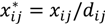 and
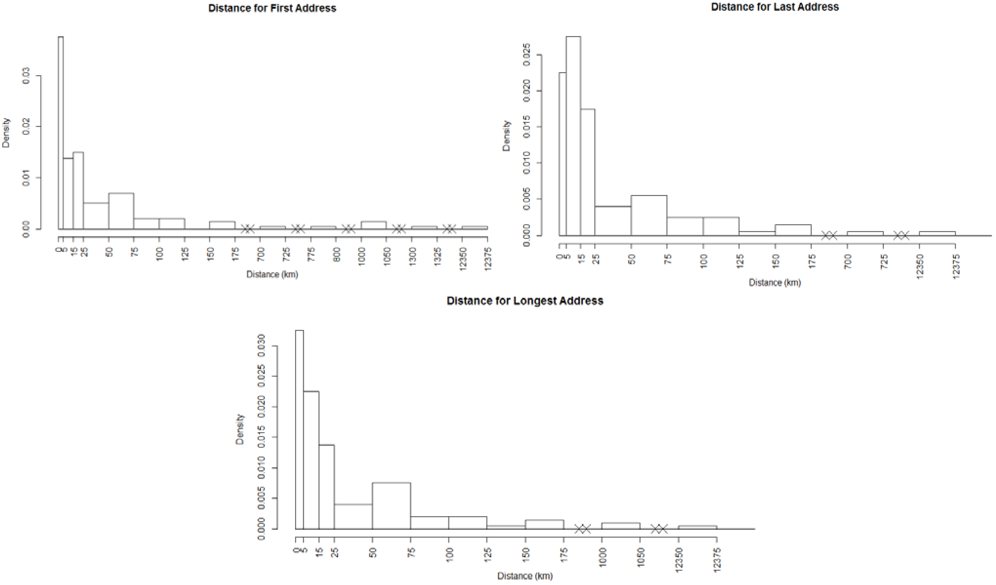
and 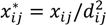 , where dij is the distance from the residential address of the participant to the sample site of the chemical calculated using the spherical law of cosines. Note that this distance can vary depending on whether the first, longest or last address is used. This transformation represents an inverse linear and inverse quadratic weighting of the variables. Figure 3 displays the histograms of the distance distributions for each address class (first, longest, and last). All chemicals were transformed in this way prior to all subsequent analysis.
 | Distance | Distance Squared | |||
|---|---|---|---|---|
| No. of Comps | Loading | No. of Comps | Loading | |
| First Address | ||||
| S | 1 | 1: mercury(−), lead(−), dintolu(−), dintolu26(−), atrazine(−), tribenz(−), dibenz(−) | 1 | 1: mercury(−), dintolu(−), dintolu26(−), atrazine(−), tribenz(−), dibenz(−) |
| W | 1 | 1: Arsenic(−), Lead(−) | 1 | 1: Arsenic(−), Lead(−) |
| S+W | 2 | 1: all negative except leadW didn’t load at all 2: mercury S(−), arsenicS(−), triCES(−), tetraCE(−), triCE112(−), acetone(−), endo2S(−), endo1S(−), tolueneS(−), DDTS(−), mercuryW(+), arsenicW(+), leadW(+), endo2W(+), endo1W(+), DDTW(+), endosulfW(+) | 2 | 1: all negative except leadW didn’t load at all 2: mercury S(−), arsenicS(−), leadS(−), tetraCES(−), triCES(-), triCE112S(−), acetoneS(−), endo2S(−), endo1S(−), tolueneS(−), DDTS(−), mercuryW(+), arsenicW(+), leadW(+), endo2W(+), endo1W(+), DDTW(+), endosulfW(+) |
| Longest Address | ||||
| S | 2 | 1: mercury(−), dintolu(−), atrazine(−), tribenz(−), dibenz(−) 2: mercury(−), lead(−), dintolu(+), dintolu26(−), atrazine(−), tribenz(−), dibenz(−) | 2 | 1: mercury(−), lead(−), dintolu(−), dintolu26(−), atrazine(−), tribenz−), dibenz(−) 2: lead(−), dintolu(−), dintolu26(−), atrazine(−), tribenz(−), dinbenz(−) |
| W | 1 | 1: Arsenic(−), Lead(−) | 1 | 1: Arsenic(−), Lead(−) |
| S+W | 2 | 1: all negative except leadW didn’t load at all 2: mercury S(−), tetraCES(+), triCES(+), dintoluS(−), endo2S(+), endo1S(+), tolueneS(−), DDTS(+), mercuryW(−), arsenicW(−), leadW(−), acetoneW(+), endo2W(−), endo1W(−), DDTW(−), endosulfW(−) | 1 | 1: all negative except leadW didn’t load at all |
| Last Address | ||||
| S | 2 | 1: mercury(−), lead(−), dintolu(−), atrazine(−), tribenz(−), dibenz(−) 2: mercury(−), lead(−), dintolu(+), atrazine(−), tribenz(−), dibenz(−) | 2 | 1: mercury(−), lead(−),dintolu(−), atrazine(−), tribenz(−), dibenz(−) 2: mercury(−), lead(−),dintolu(+), atrazine(−), tribenz(−), dibenz(−) |
| W | 1 | 1: Arsenic(−), Lead(−) | 1 | 1: Arsenic(−), Lead(−) |
| S+W | 2 | 1: all negative 2: mercuryS(−), arsenicS(−), leadS(−), dintoluS(+), tolueneS(+),artrazineS(−),dibenzS(−), mercuryW(+), arsenicW(+), leadW(+), acetoneW(−), endo2W(+), endo1W(+), tolueneW(−), DDTW(+),endosulfW(+) | 2 | 1: all loaded negative 2: mercury S(−), arsenicS(−), leadS(−), triCES(−), tetraCES(−), acetoneS(+), dintoluS(+),endo2S(+), endo1S(+), tolueneS(+), DDTS(+), mercuryW(+), arsenicW(+), leadW(+), acetoneW(−), endo2W(+), endo1W(+), tolueneW(−), DDTW(+), endosulfW(+) |
| Distance | Distance Squared | |||
|---|---|---|---|---|
| Parameter | Inclusion Probability Mean (sd) | Parameter | Inclusion Probability Mean (sd) | |
| First Address | ||||
| PCA | ||||
| Soil | Rnd(id2) | 0.326 (0.469) | Rnd(id2) | 0.334 (0.472) |
| GW | Rnd(id2) | 1.000 (0.000) | Educ | 0.337 (0.473) |
| --- | --- | Rnd(id2) | 0.668 (0.471) | |
| Joint | Rnd(id2) | 0.334 (0.472) | Rnd(id2) | 0.667 (0.471) |
| Chemical | ||||
| Soil | NULL | Rnd(id2) | 0.667 (0.471) | |
| GW | Rnd(id2) | 0.334 (0.472) | Rnd(id2) | 0.334 (0.472) |
| Joint | Rnd(id2) | 0.667 (0.471) | Rnd(id2) | 0.667 (0471) |
| Longest Address | ||||
| PCA | ||||
| Soil | Rnd(id2) | 0.667 (0.471) | Rnd(id2) | 0.667 (0.471) |
| GW | Rnd(id2) | 0.334 (0.472) | Rnd(id2) | 0.334 (0.472) |
| Joint | Rnd(id2) | 0.667 (0.471) | Rnd(id2) | 1.000 (0.000) |
| Chemical | ||||
| Soil | Rnd(id2) | 1.000 (0.00) | tetraCE | 0.346 (0.476) |
| --- | --- | Educ | 0.334 (0.472) | |
| --- | --- | Rnd(id2) | 0.334 (0.472) | |
| GW | Biphen | 0.294 (0.456) | Rnd(id2) | 0.667 (0.471) |
| Rnd(id2) | 0.334 (0.472) | --- | --- | |
| Joint | AtrazineW | 0.334 (0,472) | tribenzS | 0.334 (0.472) |
| Rnd(id2) | 0.334 (0,472) | Educ | 0.334 (0.472) | |
| --- | --- | Rnd(id2) | 0.334 (0.472) | |
| Last Address | ||||
| PCA | ||||
| Soil | Rnd(id2) | 0.334 (0.472) | Rnd(id2) | 0.667 (0.471) |
| GW | Rnd(id2) | 1.000 (0.000) | Rnd(id2) | 0.334 (0.472) |
| Joint | Rnd(id2) | 0.667 (0.471) | Rnd(id2) | 0.667 (0.472) |
| Chemical | ||||
| Soil | Atrazine | 0.334 (0.472) | Rnd(id2) | 0.667 (0.471) |
| Rnd(id2) | 0.334 (0.472) | --- | --- | |
| GW | Rnd(id2) | 0.334 (0.472) | Rnd(id2) | 1.000 (0.000) |
| Joint | Rnd(id2) | 0.667 (0.471) | NULL | NULL |
| Birth Address | Longest Address | Last Address | ||||
|---|---|---|---|---|---|---|
| Parameter | Inclusion probability Mean (sd) | Parameter Estimate Mean (95% CI) | Inclusion probability Mean (sd) | Parameter Estimate Mean (95% CI) | Inclusion probability Mean (sd) | Parameter Estimate Mean (95% CI) |
| Age | --- | --- | --- | --- | 0.5585 (0.4966) | −3.049 (−10.56, 0.203) |
| dheatG | --- | --- | --- | --- | 0.5540 (0.4971) | −3.575 (−14.94, 3.881) |
| tPaint | --- | --- | --- | --- | 0.5796 (0.4936) | −2.413 (−15.5, 6.809) |
| tTermites | 0.5664 (0.4956) | −2.507 (−15.31, 8.914) | 0.7076 (0.4549) | −4.307 (−18.04, 8.093) | --- | --- |
| Cr | 0.6298 (0.4829) | 4.739 (0.005, 15.81) * | --- | --- | --- | --- |
| Cu | 0.6426 (0.4792) | −2.377 (−8.386, −241) * | --- | --- | --- | --- |
| As | --- | --- | 0.6166 (0.4862) | 0.862 (−13.76, 14.56) | --- | --- |
| Mn | --- | --- | 0.7096 (0.4540) | 0.116 (−650, 1.054) | --- | --- |
| Pb | --- | --- | --- | --- | 0.6098 (0.4878) | 2.844 (0.320, 9.006) * |
7. Discussion and Conclusions
Acknowledgments
Author Contributions
Conflicts of Interest
References
- Somers, E.C.; Marder, W.; Cagnoli, P.; Lewis, E.E.; Deguire, P.; Gordon, C.; Helmick, C.G.; Wang, L.; Wing, J.J.; Dhar, J.P.; et al. Population-based incidence and prevalence of systemic lupus erythematosus: The michigan lupus epidemiology & surveillance (miles) program. Arthritis Rheum. 2013, 66, 357–368. [Google Scholar]
- Lim, S.S.; Bayakly, A.R.; Helmick, C.G.; Gordon, C.; Easley, K.A.; Drenkard, C. The incidence and prevalence of systemic lupus erythematosus, 2002–2004: The georgia lupus registry. Arthritis Rheum. 2014, 66, 357–368. [Google Scholar] [CrossRef]
- Miller, F.W.; Alfredsson, L.; Costenbader, K.H.; Kamen, D.L.; Nelson, L.M.; Norris, J.M.; de Roos, A.J. Epidemiology of environmental exposures and human autoimmune diseases: Findings from a national institute of environmental health sciences expert panel workshop. J. Autoimmun. 2012, 39, 259–271. [Google Scholar] [CrossRef]
- Alarcon-Segovia, D.; Alarcon-Riquelme, M.E.; Cardiel, M.H.; Caeiro, F.; Massardo, L.; Villa, A.R.; Pons-Estel, B.A. Familial aggregation of systemic lupus erythematosus, rheumatoid arthritis, and other autoimmune diseases in 1,177 lupus patients from the gladel cohort. Arthritis Rheum. 2005, 52, 1138–1147. [Google Scholar] [CrossRef]
- Kamen, D.L.; Barron, M.; Parker, T.M.; Shaftman, S.R.; Bruner, G.R.; Aberle, T.; James, J.A.; Scofield, R.H.; Harley, J.B.; Gilkeson, G.S. Autoantibody prevalence and lupus characteristics in a unique African American population. Arthritis Rheum. 2008, 58, 1237–1247. [Google Scholar] [CrossRef]
- Bruner, B.F.; Guthridge, J.M.; Lu, R.; Vidal, G.; Kelly, J.A.; Robertson, J.M.; Kamen, D.L.; Gilkeson, G.S.; Neas, B.R.; Reichlin, M.; et al. Comparison of autoantibody specificities between traditional and bead-based assays in a large, diverse collection of patients with systemic lupus erythematosus and family members. Arthritis Rheum. 2012, 64, 3677–3686. [Google Scholar] [CrossRef]
- Cooper, G.S.; Miller, F.W.; Pandey, J.P. The role of genetic factors in autoimmune disease: Implications for environmental research. Environ. Health Persp. 1999, 107, 693–700. [Google Scholar]
- Spruill, I.; Leite, R.S.; Fernandes, J.; Kamen, D.L.; Ford, M.E.; Jenkins, C.; Hunt, K.; Andrews, J. Successm challenges, and lessons learned: Community-engaged research with South Carolinas’ gullah population. Int. J. Commun. Res. Engagem. 2013, 6, 150–169. [Google Scholar]
- Arbuckle, M.R.; McClain, M.T.; Rubertone, M.V.; Scofield, R.H.; Dennis, G.J.; James, J.A.; Harley, J.B. Development of autoantibodies before the clinical onset of systemic lupus erythematosus. N. Engl. J. Med. 2003, 349, 1526–1533. [Google Scholar] [CrossRef]
- Williams, E.M.; Crespo, C.J.; Dorn, J. Inflammatory biomarkers and subclinical atherosclerosis in African American women with Systemic Lupus Erythematosus (SLE): The breakfast with a buddy biomarkers of lupus study. J. Health Disp. Res. Pract. 2009, 3, 53–70. [Google Scholar]
- Williams, E.M.; Tumiel-Berhalter, L.; Anderson, J.; Crespo, C.; Hassan, R.; Ortiz, K.; Vena, J. The Buffalo Lupus Project: A Community-based Participatory Research Investigation of Toxic Waste Exposure and Lupus. In Health Disparities among Under-served Populations: Implications for Research, Policy, and Praxis; Emerald Group Publishing Limited: West Yorkshire, UK, 2012; Volume 9, pp. 159–175. [Google Scholar]
- Williams, E.M.; Watkins, R.; Anderson, J.; Tumiel-Berhalter, L.A. Geographic information assessment of exposure to a toxic waste site and development of Systemic Lupus Erythematosus (SLE): Findings from the Buffalo lupus project. J. Toxicol. Environ. Health Sci. 2011, 3, 52–64. [Google Scholar]
- Williams, E.M.; Zayas, L.E.; Anderson, J.; Ransom, A. Reflections on lupus and the environment in an urban African American community. Humanity Soc. 2009, 33, 5–17. [Google Scholar] [CrossRef]
- Geochemistry of Soils from the PLUTO Database. Available online: http://mrdata.usgs.gov/pluto/soil (accessed on 19 December 2013).
- Aelion, C.M.; Davis, H.T.; Liu, Y.; Lawson, A.B.; McDermott, S. Validation of Bayesian kriging of arsenic, chromium, lead and mercury in surface soils concentrations based on internode sampling. Environ. Sci. Technol. 2009, 4432–4438. [Google Scholar]
- Joliffe, I. Principal Component Analysis; Springer: New York, NY, USA, 2002. [Google Scholar]
- Scheipl, F. Spikeslabgam: Bayesian variable selection, model choice and regularization for generalized additive mixed models in R. J. Stat. Softw. 2011, 43, 1–24. [Google Scholar]
- Barbieri, M.M.; Berger, J.O. Optimal predictive model selection. Ann. Statist. 2004, 32, 870–897. [Google Scholar] [CrossRef]
- Banerjee, S.; Carlin, B.; Gelfand, A. Hierarchical Modeling and Analysis for Spatial Data; CRC Press: New York, NY, USA, 2004. [Google Scholar]
- Fahrmeir, L.; Kneib, T. Bayesian Smoothing and Regression for Longitudinal Spatial and Event History Data; Oxford University Press: New York, NY, USA, 2011. [Google Scholar]
- Aelion, C.M.; Davis, H.T.; McDermott, S.; Lawson, A.B. Metal concentrations in rural topsoil in South Carolina: Potential for human health impact. Sci. Total Environ. 2008, 402, 149–156. [Google Scholar] [CrossRef]
- Davis, H.T.; Aelion, C.M.; McDermott, S.; Lawson, A.B. Identifying natural and anthropogenic sources of metals in urban and rural soils using Gis-based data, PCA, and spatial interpolation. Environ. Pollut. 2009, 2378–2385. [Google Scholar]
- George, E.I.; McCulloch, R.E. Variable selection via Gibbs sampling. J. Am. Stat. Assoc. 1993, 398–409. [Google Scholar]
- Kim, J.; Lawson, A.B.; McDermott, S.; Aelion, C.M. Variable selection for for spatial random field predictors under a reduced rank bayesian hierarchical spatial model. Spat. Spatiotemporal Epidemiol. 2009, 1, 95–102. [Google Scholar] [CrossRef]
© 2014 by the authors; licensee MDPI, Basel, Switzerland. This article is an open access article distributed under the terms and conditions of the Creative Commons Attribution license (http://creativecommons.org/licenses/by/3.0/).
Share and Cite
Carroll, R.; Lawson, A.B.; Voronca, D.; Rotejanaprasert, C.; Vena, J.E.; Aelion, C.M.; Kamen, D.L. Spatial Environmental Modeling of Autoantibody Outcomes among an African American Population. Int. J. Environ. Res. Public Health 2014, 11, 2764-2779. https://doi.org/10.3390/ijerph110302764
Carroll R, Lawson AB, Voronca D, Rotejanaprasert C, Vena JE, Aelion CM, Kamen DL. Spatial Environmental Modeling of Autoantibody Outcomes among an African American Population. International Journal of Environmental Research and Public Health. 2014; 11(3):2764-2779. https://doi.org/10.3390/ijerph110302764
Chicago/Turabian StyleCarroll, Rachel, Andrew B. Lawson, Delia Voronca, Chawarat Rotejanaprasert, John E. Vena, Claire Marjorie Aelion, and Diane L. Kamen. 2014. "Spatial Environmental Modeling of Autoantibody Outcomes among an African American Population" International Journal of Environmental Research and Public Health 11, no. 3: 2764-2779. https://doi.org/10.3390/ijerph110302764
APA StyleCarroll, R., Lawson, A. B., Voronca, D., Rotejanaprasert, C., Vena, J. E., Aelion, C. M., & Kamen, D. L. (2014). Spatial Environmental Modeling of Autoantibody Outcomes among an African American Population. International Journal of Environmental Research and Public Health, 11(3), 2764-2779. https://doi.org/10.3390/ijerph110302764