3.2. Genome-Wide Association Studies (GWAS) with Longitudinal Data for Eight Phenotypes
Table 1 and
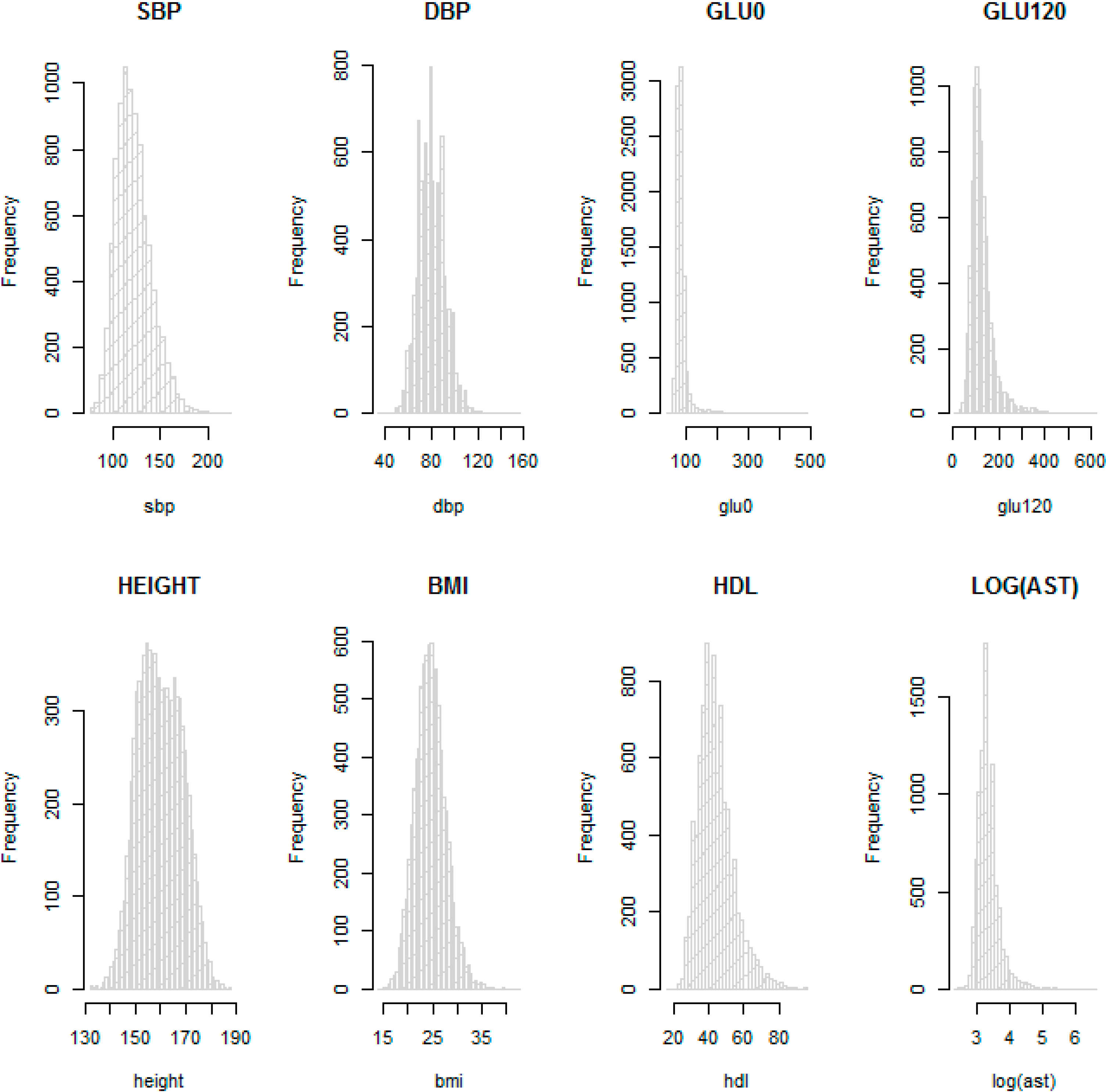
Table 2 provide descriptive statistics for sex, age and other available phenotypes from the KARE and HEXA cohorts. These show that the distributions of phenotypes are similar in the HEXA cohort the KARE cohort at each time point. We checked the normality of the eight phenotypes with histograms. In particular, AST was not normally distributed and so was log-transformed.
Figure 3 shows that log-transformed AST and the other seven phenotypes on the original scale are about normally distributed, so these were used for the GWAS.
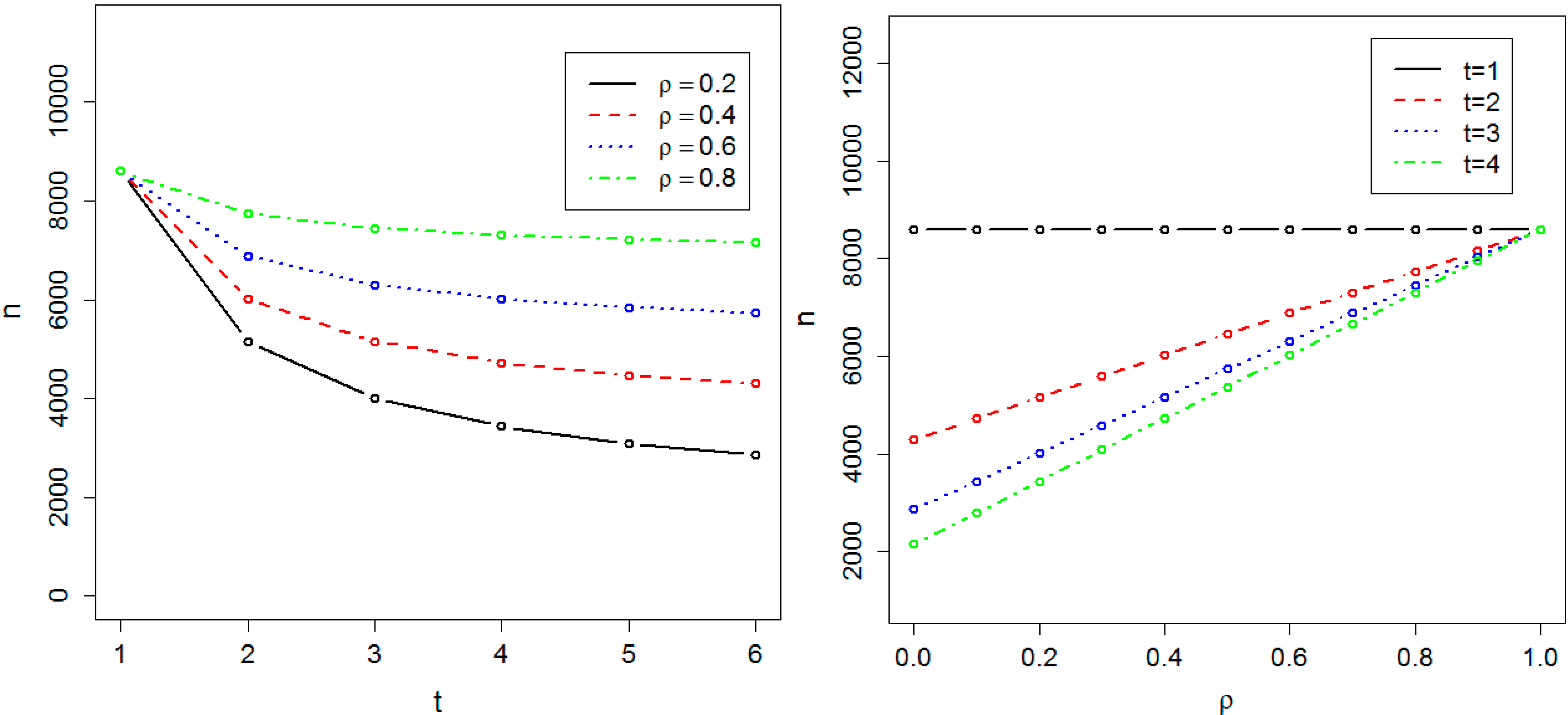
Figure 2.
Required sample size in the presence of population substructure. The sample size is indicated by n. The required sample size to achieve 0.8 power at the significance level α = 10−8 has been calculated as a function of t, the number of time points, and ρ, the correlation between measurements at two different time-points.
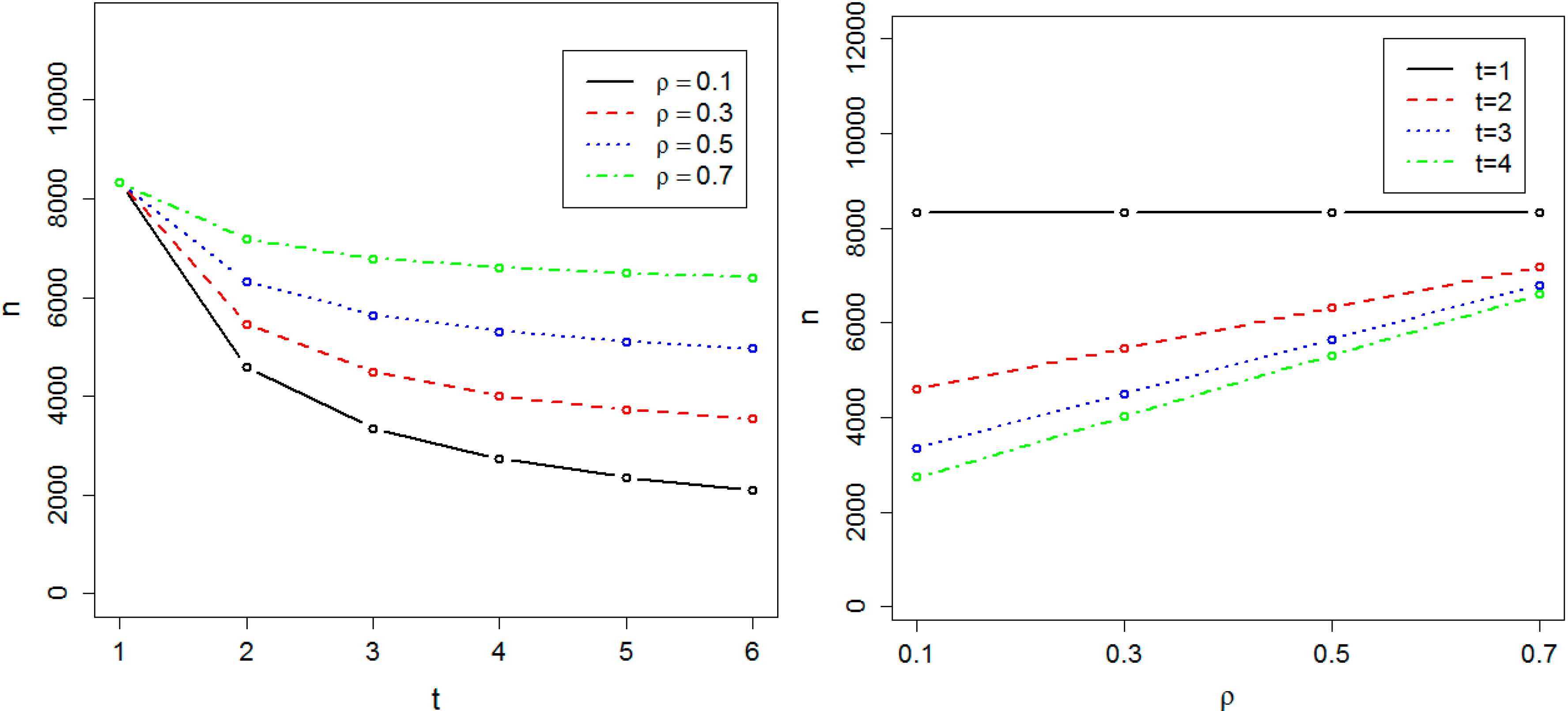
Table 1.
Sample sizes for Korean Association Resource (KARE) cohort.
Table 1.
Sample sizes for Korean Association Resource (KARE) cohort.
| Time Point | KARE |
|---|
| 1 | 2 | 3 |
|---|
| N(Ansan/Ansung) | Age(s.d) | N(Ansan/Ansung) | Age(s.d) | N(Ansan/Ansung) | Age(s.d) |
|---|
| Male | 2374/1809 | 51.78(8.79) | 1967/1642 | 53.71(8.82) | 1758/1424 | 55.58(8.71) |
| Female | 2263/2396 | 52.61(9.02) | 1764/2213 | 54.60(8.99) | 1543/1950 | 56.48(8.90) |
| Total | 4637/4205 | 52.22(8.92) | 3731/3855 | 54.18(8.92) | 3301/3374 | 56.05(8.82) |
Table 2.
Descriptive statistics for eight quantitative phenotypes examined in the Korean Association Resource (KARE) and Health Examinee (HEXA) cohorts.
Table 2.
Descriptive statistics for eight quantitative phenotypes examined in the Korean Association Resource (KARE) and Health Examinee (HEXA) cohorts.
| Time Point | KARE Cohort | HEXA Cohort |
|---|
| 1 | 2 | 3 |
|---|
| Phenotype | Mean(s.d) | N | Mean(s.d) | N | Mean(s.d) | N | Mean(s.d) | N |
| SBP | 121.65(18.61) | 8842 | 118.6(17.3) | 7504 | 116.6(16.62) | 6646 | 121.69(14.36) | 3703 |
| DBP | 80.26(11.46) | 8842 | 78.49(10.96) | 7504 | 77.69(10.25) | 6646 | 77.05(9.84) | 3703 |
| GLU0 | 87.66(21.88) | 8581 | 92.74(15.14) | 6688 | 92.31(15.15) | 5985 | 94.10(24.56) | 3703 |
| GLU120 | 126.76(51.03) | 8387 | 125.77(41.59) | 4865 | 134.07(50.56) | 5985 | Not available | |
| height | 160(8.67) | 8842 | 159.93(8.74) | 7461 | 159.95(8.76) | 6596 | 161.49(8.10) | 3703 |
| BMI | 24.6(3.12) | 8838 | 24.59(3.09) | 7456 | 24.52(3.05) | 6596 | 23.96(2.88) | 3703 |
| HDL | 44.65(10.09) | 8841 | 46.27(9.90) | 7495 | 44.04(10.25) | 6640 | 54.60(13.27) | 3703 |
| AST | 29.81(18.41) | 8841 | 24.67(14.95) | 7495 | 25.87(19.02) | 6640 | 24.51(12.94) | 3703 |
The results of the GWAS with longitudinal data in the KARE cohort were compared with the results from GWAS using cross-sectional data. For the cross-sectional data we used the phenotypes at the first time-point, applying linear regression. Population substructure was adjusted for with the EIGENSTRAT method, and five principal component (PC) scores were included as covariates in both the longitudinal and cross-sectional data analyses. We found that five PC scores explain roughly 75% of the kinship matrix, and
Table 3 shows the estimated variance inflation factors, λ, obtained by genomic control [
17]. The estimated variance inflation factors from the longitudinal data analyses were always slightly larger than those from the cross-sectional data analyses, which suggests that longitudinal data analysis tends to be more sensitive to population substructure. Even though more detailed sensitivity analyses are necessary to confirm whether the model assumption for longitudinal data analyses are satisfied, our findings are probably not affected by population substructure because the quantile-quantile (QQ) and Manhattan plots for the eight phenotypes in
Supplementary Figures 1–4 consistently show the validity of our analysis.
Figure 3.
Histograms for SBP, DBP, GLU0, GLU120, HEIGHT, BMI, HDL and log AST in the KARE cohort.
Figure 3.
Histograms for SBP, DBP, GLU0, GLU120, HEIGHT, BMI, HDL and log AST in the KARE cohort.
Table 3.
Inflation factors by genomic control.
Table 3.
Inflation factors by genomic control.
| Phenotype | Cross-Sectional Data | Longitudinal Data |
|---|
| SBP | 1.040 | 1.051 |
| DBP | 1.028 | 1.053 |
| GLU0 | 1.022 | 1.026 |
| GLU120 | 1.026 | 1.037 |
| height | 1.069 | 1.071 |
| BMI | 1.046 | 1.052 |
| HDL | 1.034 | 1.039 |
| log AST | 1.023 | 1.030 |
We calculated the correlations between the different time-points for each phenotype and they are presented in
Table 4. The correlations for height and BMI are usually very large and those for log AST are the smallest. Therefore, the improvement in power on using longitudinal data is expected to be the most substantial for log AST, and it seems to be almost negligible for height and BMI.
Table 5 and
Table 6 show the results from GWAS using longitudinal data and cross-sectional data in the KARE cohort, and the significant results were further tested in the HEXA cohort. The cross-sectional data for the KARE cohort are the first measurements for each individual in the longitudinal data. Cross-sectional and longitudinal data in the KARE cohort were analyzed with linear regression and a linear mixed model, respectively, and SNPs with
p-values from either the cross-sectional or longitudinal data analysis less than 10
−6 were selected for the replication studies. For the discovery analyses, the genome-wide significance level by Bonferroni correction is 1.4E − 07. For replication, we calculated the one-sided
p-value for the direction from the longitudinal analysis using the KARE data, and used 0.05 as the significance level. Whenever the results from the two cohorts were in different directions, the
p-values from the HEXA cohort were larger than 0.5. In
Table 5 and
Table 6, we added results from previous studies. If a SNP has not been significantly reported but SNPs in genes in linkage disequilibrium with it have been significantly reported, those SNPs are denoted by “*”.
Table 5 and
Table 6 show that GWAS using the longitudinal data in the KARE cohort identified 29 significant SNPs, 20 of which have been reported in previous GWAS, while the cross-sectional data identified only 19 genome-wide significant SNPs. Therefore we can conclude that the longitudinal data lead to substantial power improvement. In our GWAS using the longitudinal data, nine SNPs were newly detected, six of which were significantly replicated in the HEXA cohort.
Table 4.
Correlations between different time-points for each phenotype.
Table 4.
Correlations between different time-points for each phenotype.
| Time point Phenotype | Correlation between time-points |
|---|
| 1–2 | 2–3 | 1–3 |
|---|
| SBP | 0.608 | 0.604 | 0.552 |
| DBP | 0.550 | 0.596 | 0.517 |
| GLU0 | 0.700 | 0.795 | 0.822 |
| GLU120 | 0.675 | 0.748 | 0.715 |
| height | 0.984 | 0.985 | 0.984 |
| BMI | 0.942 | 0.941 | 0.916 |
| HDL | 0.690 | 0.684 | 0.667 |
| log AST | 0.444 | 0.432 | 0.468 |
Table 5 shows that rs2401887 located in CALM1 is more significantly associated with SBP in the longitudinal data analysis. GWAS of DBP identified three significant SNPs; rs3025047 in the VEGFA gene, rs7100467 near SORCS1 and rs11067763 near MED13L. It has been reported that VEGFA is related to type-2 diabetes, coronary artery disease, age-related macular degeneration and body fat [
19,
20,
21]. For GLU0, rs12991703 located near the MARCO gene was genome-wide significant using the cross-sectional data, and rs2191346 and rs6494306, which are respectively in linkage disequilibrium with DGKB and VPS13C, were more significant using the longitudinal data.
rs7197218 in the XYLT1 gene, which is related to corneal astigmatism [
22], was genome-wide significant using the cross-sectional data. rs6031492, located in GDAPL1L, is more significantly associated with GLU120 in the cross-sectional data analysis.
Table 6 shows that we detected rs17178527 in AK097143 and rs11000212 in ANAPC16 as associated with BMI. rs12292858 in SIK3 was more significant using the cross-sectional data, and rs2238153 in ATXN2, rs11066280 in HECTD4 and rs183786 near ALDH1A2 were more significantly associated with HDL by longitudinal data analysis. ATXN2, HECTD4 and ALDH1A2 have been reported to have significant associations for phenotypes related to HDL [
12,
23,
24,
25,
26,
27,
28,
29,
30,
31,
32,
33,
34], and the significant associations for HECTD4 and ALDH1A2 were successfully replicated in the HEXA cohort. We also performed GWAS of log-transformed AST, and
Table 6 shows nine significant SNPs, rs9837421 in SH3BP5, rs10849915 in CCDC63, rs3782889 in MYL2, rs12229654 near MYL2-CUX2, rs11066280 in HECTD4, rs11066453 in OAS1, rs2072134 in OAS3, rs12483959 in PNPLA3 and rs2143571 in SAMM50. Previous studies have reported that SH3BP5, CCDC63, MYL2 and OAS3 are related to alcohol dependence phenotypes [
35,
36,
37], and PNPLA3 and SAMM50 are related to nonalcoholic fatty liver disease [
38,
39], and so our results strengthen their importance in liver disease.
We also performed association analysis to detect gene×environment interaction, and SNPs that interact with aging, sex and time interval were identified by using the longitudinal data in the KARE cohort.
Table 7 and
Table 8 list SNPs with
p-values for gene×environment interaction less than 10
−6.
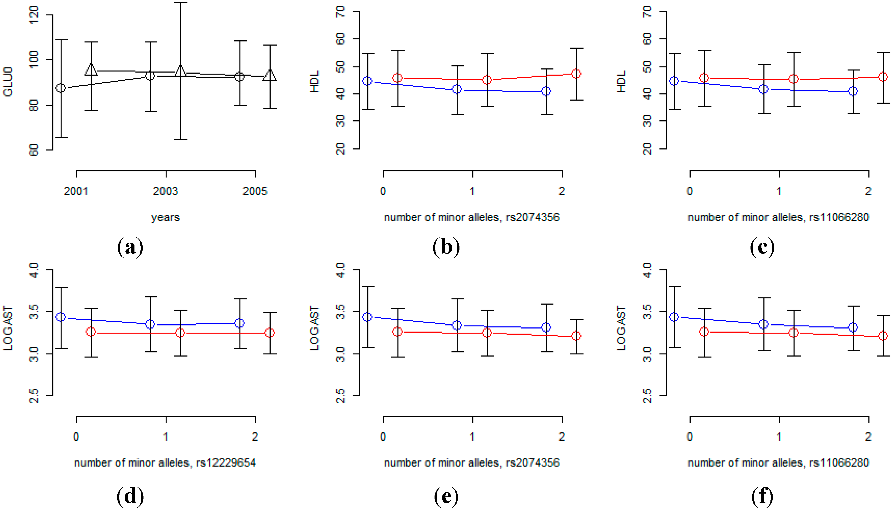
Table 7 shows that rs7197218 seems to be a promising candidate SNP for interaction with aging for GLU0, and
Figure 4 shows that the age effects are substantially different for this SNP. However, the MAF of rs7197218 is 0.01456, and neither it nor any other SNPs that are in linkage disequilibrium with it, were found in the HEXA cohort. Thus the significant association of this SNP could not be confirmed and it will need to be further investigated in follow-up studies.
Table 8 shows that rs2074356 and rs11066280 interact significantly with sex for HDL, and rs2074356, rs11066280 and rs12229654 do so for log-transformed AST. Interestingly, rs2074356 and rs11066280 have significant interaction effects with sex for both HDL and AST. We further confirmed these significant gene×environment interactions in the HEXA cohort. Based on the direction of the coefficients for these interactions, we calculated one-sided
p-values, and the combined
p-values by Fisher’s and Liptak’s methods [
40,
41]. It has been shown that the most efficient method is achieved by Liptak’s methods if the effect sizes are expected to be the same [
42].
Table 9 shows that these significant interactions were further replicated in the HEXA cohort, and the combined
p-values become smaller.
Figure 4 shows that the effects of these SNPs are substantially different for males and females and, therefore, we can conclude that the effects of these SNPs are significantly different for males and females.
In summary, we can conclude that GWAS with longitudinal data provide an efficient strategy, and our overall results show that the improvement in power is substantial, its effect being inversely proportional to ρ.
Table 5.
Results for SBP, DBP, GLU0 and GLU120. SNPs with p-values less than 10−6 from cross-sectional or longitudinal data are listed.
Table 5.
Results for SBP, DBP, GLU0 and GLU120. SNPs with p-values less than 10−6 from cross-sectional or longitudinal data are listed.
| SNP | Chr | Position | Nearby Gene | Minor Allele | MAF | Discovery | Replication | Previously Published |
|---|
| Cross-Sectional | Longitudinal | Cross-Sectional |
|---|
| beta ± s.e | P | beta ± s.e | P | beta ± s.e | one-side P |
|---|
| SBP |
| rs17249754 | 12 | 88584717 | ATP2B1 | A | 0.3732 | −1.63 ± 0.27 | 9.73E − 10 | −1.27 ± 0.22 | 1.11E − 08 | −0.86 ± 0.49 | 5.30E − 03 | Cho et al. NG 2009 [11] |
| rs11066280 | 12 | 111302166 | in HECTD4 | T | 0.1717 | −1.45 ± 0.34 | 2.52E − 05 | −1.59 ± 0.29 | 2.95E − 08 | −1.65 ± 0.43 | 6.35E − 05 | Kato et al. NG 2011 [27] |
| rs2401887 | 14 | 89952963 | CALM1 | C | 0.02125 | −3.19 ± 0.93 | 5.89E − 04 | −3.84 ± 0.78 | 8.58E − 07 | | | |
| DBP |
| rs10030362 | 4 | 102841866 | in BANK1 | C | 0.2081 | −0.72 ± 0.21 | 4.34E − 04 | −0.87 ± 0.17 | 3.21E − 07 | −0.22 ± 0.27 | 2.11E-01 | * Zhang et al. Hypertension Res 2012 [43] |
| rs3025047 | 6 | 43854388 | in VEGFA | A | 0.01024 | −2.65 ± 0.2 | 1.75E − 03 | −3.64 ± 0.71 | 3.07E − 07 | | | |
| rs7100467 | 10 | 108153198 | SORCS1 | T | 0.02356 | −2.43 ± 0.53 | 1.81E − 04 | −2.82 ± 0.55 | 3.43E − 07 | | | |
| rs17249754 | 12 | 88584717 | ATP2B1 | A | 0.3732 | −0.94 ± 0.17 | 4.33E − 08 | −0.8 ± 0.14 | 2.01E − 08 | −0.56 ± 0.23 | 8.50E − 03 | Cho et al. NG 2009 [11] |
| rs11066280 | 12 | 111302166 | in HECTD4 | T | 0.1717 | −0.94 ± 0.22 | 1.97E − 05 | −0.98 ± 0.18 | 9.25E − 08 | −0.76 ± 0.38 | 5.35E − 03 | Kato et al. NG 2011 [27] |
| rs11067763 | 12 | 114682724 | MED13L | G | 0.3297 | −0.78 ± 0.18 | 1.04E − 05 | −0.79 ± 0.15 | 8.75E − 08 | 0 ± 0.35 | 5.04E − 01 | |
| GLU0 |
| rs12991703 | 2 | 119536716 | MARCO | A | 0.05655 | 3.62 ± 0.68 | 1.18E − 07 | 2.51 ± 0.58 | 1.55E − 05 | −1.14 ± 0.7 | 9.11E − 01 | |
| rs7754840 | 6 | 20769229 | in CDKAL1 | C | 0.4761 | 1.8 ± 0.32 | 1.72E − 08 | 1.78 ± 0.27 | 5.16E − 11 | 0.98 ± 0.74 | 3.99E − 02 | Kwak et al. Diabetes 2012 [44] |
| rs9460546 | 6 | 20771611 | in CDKAL1 | G | 0.4808 | 1.75 ± 0.32 | 3.38E − 08 | 1.76 ± 0.27 | 3.76E − 11 | | | |
| rs2191346 | 7 | 15020403 | DGKB | C | 0.2891 | −1.72 ± 0.36 | 1.33E − 06 | −1.53 ± 0.3 | 3.64E − 07 | −0.62 ± 0.62 | 1.55E − 01 | |
| rs6494306 | 15 | | VPS13C | A | 0.3435 | −1.43 ± 0.33 | 1.71E − 05 | −1.46 ± 0.28 | 1.92E − 07 | −1.21 ± 0.59 | 2.08E − 02 | * Manning et al. NG 2012 [45] |
| rs7197218 | 16 | 17319136 | in XYLT1 | G | 0.01456 | 7.23 ± 0.68 | 1.23E − 07 | 4.29 ± 1.17 | 2.48E − 04 |
| GLU120 |
| rs7754840 | 6 | 20769229 | in CDKAL1 | C | 0.4761 | 4.73 ± 0.78 | 1.51E − 09 | 4.73 ± 0.73 | 1.10E − 10 | | | Kwak et al. Diabetes 2012 [44] |
| rs12229654 | 12 | 109898844 | MYL2-CUX2 | G | 0.1426 | −4.84 ± 1.11 | 1.21E − 05 | −5.16 ± 1.03 | 5.84E − 07 | | | Go et al. J Hum Genet 2013 [46] |
| rs2074356 | 12 | 111129784 | in HECTD4 | T | 0.1467 | −5.19 ± 1.09 | 2.02E − 06 | −5.2 ± 1.02 | 3.44E − 07 | | | Go et al. J Hum Genet 2013 [46] |
| rs6031492 | 20 | 42330963 | in GDAPL1L | G | 0.4949 | 3.84 ± 0.77 | 6.91E − 07 | 3.03 ± 0.72 | 2.81E − 05 | | | |
| rs2868088 | 20 | 42347066 | GDAPL1L | A | 0.4377 | −3.99 ± 0.78 | 2.68E − 07 | −3.54 ± 0.72 | 1.04E − 06 | | | |
Table 6.
Results for Height, BMI, HDL and log AST. SNPs with p-values less than 10−6 from cross-sectional or longitudinal data are listed.
Table 6.
Results for Height, BMI, HDL and log AST. SNPs with p-values less than 10−6 from cross-sectional or longitudinal data are listed.
| SNP | Chr | Position | Nearby gene | Minor Allele | MAF | Discovery | Replication | Previously Published |
|---|
| Cross-sectional | Longitudinal | Cross-Sectional |
|---|
| beta ± s.e | P | beta ± s.e | P | beta ± s.e | one-side P |
|---|
| Height |
| rs17038182 | 1 | 118669928 | SPAG17 | G | 0.4188 | −0.45 ± 0.08 | 4.08E − 08 | −0.45 ± 0.08 | 5.58E − 08 | −0.13 ± 0.13 | 1.53E − 01 | Cho et al. Nat Genet 2009 [11] |
| rs10513137 | 3 | 142626120 | in ZBTB38 | A | 0.2605 | 0.49 ± 0.09 | 8.14E − 08 | 0.49 ± 0.09 | 5.85E − 08 | 0.43 ± 0.14 | 7.40E − 04 | Kim et al. J Hum Genet 2009 [47] |
| rs6918981 | 6 | 34346492 | RPL35P2-NUDT3 | G | 0.2092 | 0.55 ± 0.1 | 2.98E − 08 | 0.55 ± 0.1 | 1.72E − 08 | 0.1 ± 0.15 | 2.51E − 01 | Kim et al. J Hum Genet 2009 [47] |
| BMI |
| rs17178527 | 6 | 141947773 | in AK097143 | A | 0.2486 | −0.32 ± 0.05 | 2.96E − 09 | −0.31 ± 0.05 | 6.35E-09 | 0.05 ± 0.08 | 7.47E − 01 | |
| rs11000212 | 10 | 73625658 | in ANAPC16 in ASCC1 | G | 0.2057 | 0.27 ± 0.06 | 1.85E − 06 | 0.28 ± 0.06 | 5.14E − 07 | 0.05 ± 0.08 | 2.90E − 01 | |
| rs9939609 | 16 | 52378028 | in FTO | T | 0.1262 | 0.34 ± 0.07 | 1.29E − 06 | 0.34 ± 0.07 | 7.36E − 07 | 0.23 ± 0.1 | 1.29E − 02 | Cho et al. Nat Genet 2009 [11] |
| HDL |
| rs271 | 8 | 19857982 | in LPL | T | 0.2064 | 1.15 ± 0.19 | 4.84E − 10 | 1.12 ± 0.17 | 2.15E − 11 | 1.81 ± 0.38 | 7.70E − 07 | |
| rs17482753 | 8 | 19876926 | LPL | T | 0.1243 | 1.95 ± 0.23 | 8.83E − 18 | 1.91 ± 0.21 | 1.42E − 20 | 3.48 ± 0.46 | 2.71E − 14 | Heid et al. Circ Cardiovasc Genet 2008 [48] |
| rs17410962 | 8 | 19892360 | LPL | A | 0.1244 | 1.95 ± 0.23 | 8.25E − 18 | 1.91 ± 0.21 | 1.76E − 20 | 3.48 ± 0.46 | 2.35E − 14 | |
| rs12686004 | 9 | 106693247 | in ABCA1 | T | 0.2136 | −1.26 ± 0.2 | 7.01E − 12 | −1.37 ± 0.17 | 1.62E − 16 | −1.19 ± 0.32 | 6.10E − 04 | Kim et al. Nat Genet 2011 [12] |
| rs11216126 | 11 | 116122450 | BUD13 | C | 0.2027 | 1.43 ± 0.19 | 2.69E − 14 | 1.36 ± 0.17 | 1.54E − 15 | 1.44 ± 0.5 | 7.45E − 05 | Kim et al. Nat Genet 2011 [12] |
| rs6589566 | 11 | 116157633 | in ZNF259 | C | 0.2176 | −1.25 ± 0.18 | 1.10E − 11 | −1.15 ± 0.17 | 4.47E − 12 | −1.89 ± 0.32 | 8.15E − 08 | * Waterworth et al. Arteriosclear Thromb Vasc Biol 2010 [49] |
| rs12292858 | 11 | 116319189 | in SIK3 | C | 0.1759 | 1.05 ± 0.2 | 7.73E − 08 | 0.88 ± 0.18 | 7.68E − 07 | 0.9 ± 0.35 | 1.11E − 02 | |
| rs12229654 | 12 | 109898844 | MYL2-CUX2 | G | 0.1426 | −1.25 ± 0.24 | 6.42E − 09 | −1.21 ± 0.2 | 7.35E − 10 | −1.66 ± 0.46 | 1.25E − 04 | Kim et al. Nat Genet 2011 [12] |
| rs2238153 | 12 | 110423930 | in ATXN2 | A | 0.4579 | −0.68 ± 0.16 | 8.76E − 06 | −0.71±0.14 | 3.29E − 07 | | | |
| rs11066280 | 12 | 111302166 | in HECTD4 | T | 0.1717 | −1.4 ± 0.15 | 3.10E − 12 | −1.35±0.18 | 1.17E − 13 | −1.92 ± 0.4 | 8.95E − 07 | |
| rs2072134 | 12 | 111893559 | in OAS3 | A | 0.1143 | −1.39 ± 0.19 | 4.53E − 09 | −1.31 ± 0.22 | 1.25E − 09 | −1.36 ± 0.4 | 2.33E − 03 | Kim et al. Nat Genet 2011 [12] |
| rs183786 | 15 | 56455402 | ALDH1A2 | T | 0.305 | −0.8 ± 0.16 | 8.53E − 07 | −0.83 ± 0.15 | 2.33E − 08 | −0.61 ± 0.33 | 3.13E-02 | |
| rs16940212 | 15 | 56481312 | LIPC | T | 0.3405 | 1.27 ± 0.16 | 1.05E − 15 | 1.3 ± 0.14 | 1.95E − 19 | 1.11 ± 0.47 | 2.04E − 04 | Kim et al. Nat Genet 2011 [12] |
| rs6494005 | 15 | 56511816 | in LIPC | G | 0.2678 | −0.89 ± 0.2 | 1.34E − 07 | −0.89 ± 0.15 | 5.82E − 09 | −0.79 ± 0.39 | 1.05E − 02 | |
| rs12708980 | 16 | 55569880 | in CETP | C | 0.0984 | −1.67 ± 0.25 | 3.63E − 11 | −1.65 ± 0.23 | 5.61E − 13 | −1.88 ± 0.5 | 7.40E − 05 | Kim et al. Nat Genet 2011 [12] |
| rs2156552 | 18 | 45435666 | LIPG | A | 0.164 | −0.89 ± 0.21 | 1.53E − 05 | −0.93 ± 0.19 | 5.90E − 07 | −1.15 ± 0.4 | 2.29E − 03 | Waterworth et al. Arteriosclear Thromb Vasc Biol 2010 [49] |
| rs4420638 | 19 | 50114786 | APOC1 | C | 0.1121 | −1.3 ± 0.16 | 4.21E − 08 | −1.14 ± 0.21 | 1.23E − 07 | −2.01 ± 0.47 | 1.88E − 05 | Willer et al. Nat Genet 2013 [50] |
| AST |
| rs9837421 | 3 | 15322297 | in SH3BP5 | G | 0.193 | −0.02 ± 0.01 | 2.14E − 04 | −0.03 ± 0.01 | 5.79E − 07 | 0 ± 0 | 5.32E − 01 | |
| rs10849915 | 12 | 109818005 | in CCDC63 | G | 0.1758 | −0.03 ± 0.01 | 2.00E − 06 | −0.03 ± 0.01 | 1.81E − 08 | −0.02 ± 0 | 3.68E − 02 | |
| rs3782889 | 12 | 109835038 | in MYL2 | C | 0.1726 | −0.03 ± 0.01 | 3.79E − 06 | −0.03 ± 0.01 | 7.26E − 09 | −0.02 ± 0 | 2.02E − 02 | |
| rs12229654 | 12 | 109898844 | MYL2-CUX2 | G | 0.1426 | −0.04 ± 0.01 | 7.34E − 08 | −0.04 ± 0.01 | 4.74E − 11 | −0.02 ± 0 | 2.80E − 02 | |
| rs11066280 | 12 | 111302166 | in HECTD4 | T | 0.1717 | −0.05 ± 0.01 | 8.17E − 13 | −0.05 ± 0.01 | 1.70E − 18 | −0.03 ± 0 | 1.94E − 04 | |
| rs11066453 | 12 | 111850004 | in OAS1 | G | 0.1265 | −0.03 ± 0.01 | 5.26E − 06 | −0.03±0.01 | 8.72E − 07 | −0.02 ± 0 | 7.75E − 02 | |
| rs2072134 | 12 | 111893559 | in OAS3 | A | 0.1143 | −0.04 ± 0.01 | 7.31E − 08 | −0.04 ± 0.01 | 8.42E − 09 | −0.02 ± 0 | 6.75E − 02 | |
| rs12483959 | 22 | 42657329 | in PNPLA3 | A | 0.4157 | 0.03 ± 0 | 1.79E − 09 | 0.03 ± 0 | 1.02E − 12 | 0.03 ± 0 | 2.14E − 06 | * Kamatani et al. Nat Genet 2010 [38] |
| rs2143571 | 22 | 42723019 | in SAMM50 | T | 0.4136 | 0.02 ± 0.01 | 6.45E − 07 | 0.03 ± 0 | 7.73E − 10 | 0.03 ± 0 | 4.22E − 05 | * Kawaguchi et al. PLoS One 2012 [39] |
Table 7.
Gene × environment interaction effect in the KARE cohort. Interactions of time interval with SNP were tested, and p-values for SNPs with genome-wide significant interaction are listed.
Table 7.
Gene × environment interaction effect in the KARE cohort. Interactions of time interval with SNP were tested, and p-values for SNPs with genome-wide significant interaction are listed.
| Effect | rs7197218 for GLU0 |
|---|
| beta | Std.Error | p-value |
|---|
| SNP | 5.92 | 1.21 | 1.08E − 06 |
| time×SNP | −1.27 | 0.25 | 2.65E − 07 |
Table 8.
Gene × environment interaction effect in the KARE cohort. Interactions of sex with SNPs were tested, and p-values for SNPs with genome-wide significant interaction are listed.
Table 8.
Gene × environment interaction effect in the KARE cohort. Interactions of sex with SNPs were tested, and p-values for SNPs with genome-wide significant interaction are listed.
| Effect | rs2074356 for HDL | rs11066280 for HDL | rs2074356 for Log(AST) | rs11066280 for Log(AST) | rs12229654 for Log(AST) |
|---|
| beta | Std.Error | p-value | beta | Std.Error | p-value | beta | Std.Error | p-value | beta | Std.Error | p-value | Beta | Std.Error | p-value |
|---|
| SNP | −4.80 | 0.62 | 7.28E − 15 | −4.69 | 0.58 | 4.60E − 16 | −0.13 | 0.02 | 5.52E − 13 | −0.17 | 0.02 | 2.81E − 20 | −0.15 | 0.02 | 1.32E − 19 |
| sex×SNP | 2.26 | 0.39 | 4.46E − 09 | 2.21 | 0.36 | 1.06E − 09 | 0.06 | 0.01 | 5.82E − 08 | 0.08 | 0.01 | 8.25E − 12 | 0.07 | 0.01 | 3.24E − 11 |
Figure 4.
Interaction effects of SNPs with sex or time interval. (a) Mean of GLU0 at each time-point for each of two rs7197218 genotypes (circles indicate homozygous genotypes with no minor alleles, triangles indicate heterozygous genotypes); (b-f) phenotypic mean of each genotype for males and females (blue and red lines indicate male and female, respectively).


