
Plant Ontogeny Strongly Influences SO2 Stress Resistance in Landscape Tree Species Leaf Functional Traits
by

Aru Han
1,2,3,4, 
Yongbin Bao
1,2,3,4,
Xingpeng Liu
1,2,3,4,
Zhijun Tong
1,2,3,4,
Song Qing
5,
Yuhai Bao
5 and
Jiquan Zhang
1,2,3,4,* 1
School of Environment, Northeast Normal University, Changchun 130024, China
2
Key Laboratory for Vegetation Ecology, Ministry of Education, Changchun 130024, China
3
State Environmental Protection Key Laboratory of Wetland Ecology and Vegetation Restoration, Changchun 130024, China
4
Jilin Province Science and Technology Innovation Center of Agro-Meteorological Disaster Risk Assessment and Prevention, Changchun 130024, China
5
College of Geographical Science, Inner Mongolia Normal University, Hohhot 010022, China
*
Author to whom correspondence should be addressed.
Remote Sens. 2022, 14(8), 1857; https://doi.org/10.3390/rs14081857
Submission received: 27 February 2022
/
Revised: 9 April 2022
/
Accepted: 10 April 2022
/
Published: 12 April 2022
(This article belongs to the Special Issue Forest Resilience to Extreme Events)
Abstract
:Sulfur dioxide (SO2) is a major atmospheric pollutant and abiotic stressor. Although physiological studies on abiotic stressors have focused on fully expanded leaves, the resistance of leaf functional traits to SO2 during individual leaf development has not been studied. Thus, this study aimed to conduct SO2 static artificial fumigation experiments to evaluate changes in leaf functional traits and resistance to SO2 for three common landscape tree species (Syringa oblata Lindl. (S. oblata), Prunus cerasifera var. atropurpurea Jack. (P. cerasifera), and Ulmus pumila ‘Jinye’ (U. pumila)) in Changchun City and ontogeny under SO2 stress. Samples were collected on three days in autumn (1 September, 9 September, and 19 September 2019) for two different leaf stages (10 days and 40 days). In addition, remote sensing data were combined to explore the resistance mechanisms of broadleaf forests to different SO2 concentration classes during different seasons on a large scale. The results showed that the chlorophyll content, leaf temperature, green-peak reflectance, and Fv/Fm (maximal photochemical efficiency) at 10 days were significantly lower than that at 40 days, regardless of sampling date or SO2 concentration. Additionally, in general the SO2 resistance for 10 days leaves was consistently smaller than those for 40 days leaves in 3 tree species. On 9 September, 10 days leaves of the three tree species showed different leaf resistance performances under different SO2 concentrations in the order: P. cerasifera > S. oblata > U. pumila. Lastly, the extent of resistance decreased with increasing ρ(SO2) classes in different seasons, and the SO2 resistance was affected by season. We conclude that mature leaves are more resistant to SO2 stress than young leaves are. These results will provide scientific guidance on artificial plant community construction and prevention of future vegetation degradation.
1. Introduction
With rapid urbanization, energy-intensive industries and factories are increasing, resulting in a larger consumption of coal than that in the past [1]. Car ownership is growing, resulting in increasing amounts of nitrogen oxides and sulfur dioxide emitted into the atmosphere. Sulfur dioxide (SO2) is a colorless and pungent pollutant that is widely distributed in the atmosphere [2]. It has a significant impact on air conditions and is responsible for increasing the acidity of rainfall. SO2 also has a serious impact on the growth of plants in cities [1,3,4,5], it hinders the development of plants, long-term exposure to sulfur dioxide will damage the epidermis of plants, weaken photosynthesis and cause injury spots on the foliage, which will gradually wither until death.
In polluted environments, sensitive plant species can act as bio-indicators of air pollution, whereas tolerant plant species can act as air pollutant sinks [6,7]. A major challenge for future research is understanding the resistance and resilience of tropical arid forests to alternating severe droughts and major storms [8]. Resistance indicators play an important role as standards in the evaluation of plant resistance to air pollution and the selection of resistant tree species. This has long been a target of research and substantial results have been achieved in this field. Currently, indicators for evaluating the resistance of plants to air pollution include leaf anatomical structure, changes in leaf fluid values and chlorophyll content, changes in cell membrane permeability, activity, and content, measures of the acute injury threshold and tolerance formula, and comprehensive evaluations of plant resistance [9,10,11,12,13,14,15,16,17,18]. These indicators can reflect the resistance and sensitivity of plants to SO2 to a certain extent. The resistance of plants to environmental stress can be affected by many factors; however, the effects of multiple factors are different [19,20]. Many researchers have comprehensively evaluated many factors to evaluate plant resistance. Currently, the comprehensive evaluation methods for plant stress resistance mainly include the membership function method, coordinated comprehensive evaluation method, and analytic hierarchy process [20,21]. These methods use statistical approaches to analyze several indices related to plant resistance and to sort the indices to determine plant resistance. A comprehensive evaluation method can accurately reflect the strength of plant resistance [19].
As an important indicator of the continuous life process of leaves from spreading through to maturation, aging, and withering, leaf age reflects the development process of plant leaves and is the scale of the length of leaf life activities. The resistance of different plants to SO2 varies greatly, as do plant species, varieties, ontogeny, tree parts, and leaf age [15,16,17,18]. Among them, plant ontogeny may be crucial and is well known in the so-called age-related resistance (ARR) [22]. ARR, also known as ontogenetic resistance, describes the ability of an entire plant or plant part to resist or tolerate diseases as it ages and matures. ARR occurs in many plant species and is usually broad-spectral [23]. Farber and Mundt [24] showed that the disease severity in young plants was significantly higher than that in old plants. The average disease severity of inoculated plants was 50.4%, 30.1%, and 12.9% for 3-week-old, 4-week-old, and 5-week-old plants, respectively. The disease severity decreased from the upper young leaves to the older lower leaves of wheat plants. Photosynthetic capacity decreases with increasing leaf age and is accompanied by an increase in leaf dry mass per unit area and a decrease in N, P, K, and Mg contents [25,26]. Gilmore [27] showed that as leaf age increased in Abies balsamea, the number of rows of viable cells in the primordia decreased, thus gradually reducing the ability of the needles to export photosynthetic products. Rapid changes in the age-class structure of boreal forests due to intensified forest use and, in some areas, due to increased natural disturbance, the proportion of old-growth forests has declined significantly, whereas that of young post-harvest and post-natural disturbance forests has increased [28].
Resistance to tropical storms and the restoration of tropical dry forests after disturbance also depends on other structural and functional characteristics [8]. Plant functional traits are a research hotspot in plant physiological and community ecology and are frequently used to predict species distributions, dynamics, and responses to environmental change [29]. Chen et al. [30] investigated a series of functional traits of the leaves and branches of 20 drought-tolerant broadleaf species planted in an arid limestone habitat in northern China. Plant ecologists have long been interested in elucidating the relationships between plant functional traits and the environment. Plant functional trait-environment relationships are the result of a combination of climatic, disturbance, and biotic conditions [31], and plants develop adaptive strategies under different environmental gradients by changing their functional traits. In addition, environmental conditions vary in communities at different successional stages, and changing environmental factors drive changes in the functional traits and ecological responses of species to adapt to the environment at the community level.
With the development of new techniques, such as infrared thermography and ground-based spectroscopy, these physiological changes can now be directly and non-destructively detected before the appearance of obvious signs of injury. Thermal infrared imaging is a promising option [32] and is based on the principle that water evapotranspiration cools and stomata close to warm leaves. Nilsson [33] predicted that the dynamic process of temperature change is important for identifying different levels of biotic or abiotic stresses. Hyperspectral remote sensing plays an important role in quantitative vegetation monitoring because of its rapid, nondestructive, and high spectral resolution [34,35]. This avoids blade damage and tedious workloads.
Therefore, this study combined biophysical methods such as spectroscopy, thermography with biochemical studies, and indoor simulated infiltration experiments to investigate variations in leaf functional traits at different ontogenies under SO2 stress and the resistance to SO2 stress. The specific objectives were as follows: (1) to investigate the changes in plant analysis development Chlorophyll content SPAD values, leaf temperature, spectral characteristics, and chlorophyll fluorescence characteristics of different tree species and ontogeny (10 days and 40 days) under SO2 stress, (2) to comprehensively evaluate the resistance of the three green tree species to SO2 at different ontogenies, and (3) to explore the resistance mechanisms of broadleaf trees to different SO2 concentration classes in different seasons on a large scale using the spatial products of fraction of photosynthetically active radiation (FPAR), gross primary productivity (GPP), and leaf area index (LAI), and normalized difference vegetation index (NDVI). Examining variations in functional traits of urban greening trees and environmental factors, as well as the response of the functional traits to environmental changes will provide a basis for the scientific guidance of artificial plant community construction and prevention of future vegetation degradation.
2. Materials and Methods
2.1. Laboratory Study on the Effect of SO2 on the Leaves of Three Common Garden Tree Species
2.1.1. Experimental Materials and Design
Taking into account the typical local greenery species, as well as aesthetically different colors and different color trees with different stomatal densities. In this study, seedlings of three different colored landscape plants (Syringa oblata Lindl. (S. oblata), Prunus cerasifera var. atropurpurea Jack. (P. cerasifera), and Ulmus pumila ‘Jinye’ (U. pumila)) commonly used in Jilin Province were selected as the research targets, and a simulated fumigation test was carried out to compare the differences in SPAD, leaf temperature, spectral characteristics, and chlorophyll fluorescence in different leaf ontogenies between the control and SO2 treatments, and to evaluate the resistance of the three plants to SO2 stress.
(1) Seedling culture
The experiment was conducted at the agriculture base facility of Jilin Agricultural University in 2019, and the experimental materials were provided by a local nursery. 1-year-old seedlings of S. oblate, U. pumila, and P. cerasifera with relatively consistent growth were selected as the experimental materials (Table 1). They were potted for monoculture in May 2019 with a pot size of 26 cm × 21 cm. The potting soil was a 3:1 mixture of garden and charcoal soil. After the potted seedlings entered the vigorous growth period in the open field, they were placed in a fumigation chamber for one week before treatment.
(2) Fumigation method
A static fumigation method was adopted [36,37], in which the fumigation device was a three-dimensional (1.5 m × 1.5 m × 1.5 m) plastic film sealed box placed outside in a windproof shed, with gas delivered through a suction tube. A 3 V fan was used to keep the air circulating in the fumigation box. Considering that the soil has a certain absorption capacity for SO2, the potted container was sealed with plastic bags during the experiment, and only the plant body was fumigated. A sulfur dioxide detector (AKBT-SO2-J, Akoote, USA) was used to monitor the SO2 in the fumigation chamber.
The SO2 contraction was kept stable. The seedlings of the three tree species were placed in three fumigation hoods, with three replicates for each SO2 concentration, and each tree species with three pots of the same age, height, basal diameter, and growth. The SO2 concentrations in the three hoods were CK (T1, control check), 7 (T2, low) and 14 (T3, high) ppm. From 19 August 2019, each plant was placed inside a fumigation chamber for one week before treatment. Then, each plant was fumigated for eight days, and fumigation was performed every two days for 3 h per day. Each index was measured at two-day intervals until the end of fumigation on 22 September 2019 when various indices were measured. After fumigation, plants were allowed to continue growing under natural conditions.
2.1.2. Experimental Measurement and Data Processing
During the autumn phenological period, sunny days before and after fumigation were selected as the days on which the various indexes would be measured. Table 2 shows the detailed schedule of the experiment.
(1) Infrared thermal imaging
Infrared thermal images were taken with an NEC H2640 (NEC Avio Infrared Technologies Co., Ltd., Tokyo, Japan) thermal infrared camera (wavelength 8–13 μm) with a temperature measurement range of −40 to 500 °C and a minimum temperature sensing capability of 0.03 °C. The ambient temperature for leaf temperature measurement was 30–31 °C. The thermal image temperature was recorded between 09:00 and 11:00, with the camera held 160 cm from the ground after focusing clearly, and then photographed under natural light. The temperature of the thermal image was then obtained from the average temperature of the entire thermal image. Finally, the thermal images and corresponding point leaf temperature values were extracted using the InfReC Analyzer NS9500 (NEC Avio Infrared Technologies Co., Ltd., Tokyo, Japan) Standard package [38]. The foliar temperature of plants (referred to as leaf temperature) is an important physiological characteristic of plants and is a fundamental parameter in the physiological and ecological research of crops [39]. The change in leaf temperature is the result of a combination of environmental and internal plant factors that affect the leaf energy balance [40]. Leaf temperature reflects the physiological state of plants and is generally believed to be related to photosynthesis. Changes in leaf temperature affect photosynthesis, and environmental conditions also have a considerable impact on leaf structure and photosynthetic characteristics [41,42]. On each date, 3 leaves were taken from 10 days leaves and 3 leaves were taken from 40 days leaves of each plant to collect infrared thermal imaging. The 18 pieces were collected for each concentration and tree species, 54 pieces for three concentrations and 162 pieces for three tree species. Collect 5 times infrared thermal imaging for each leaf, and finally take the average.
(2) Spectral reflectance of leaves
The American ASD Fieldspec4 portable ground object spectrometer was used to determine leaf spectral reflectance, with a wavelength range of 350–2500 nm and band intervals of 1.4 nm at 350–1000 nm and 1.1 nm at 1001–2500 nm. The blades were measured directly using a handheld blade clamp with an embedded standard light source (50 W) and a built-in tungsten halogen lamp. Before spectral reflectance measurements, a standard white BaSO4 panel calibration was used. During the measurement, ten curves were recorded at 0.1 s intervals, and the average value was taken. Standard white BaSO4 panel correction was performed every 15 min to ensure standardization of the different positions and zones of the leaves. Finally, the original spectral data of the leaves were extracted using View SpecPro, and the spectrometer resampled the spectral data at 1 nm intervals during the output value [43]. On each date, 3 leaves were taken from 10 days leaves and 3 leaves were taken from 40 days leaves of each plant to collect spectral curves. Eighteen pieces were collected for each concentration and tree species, 54 pieces for three concentrations and 162 pieces for three tree species. Ten spectral curves were collected for each leaf, and an average was taken.
(3) Photosynthetic parameters
A Li-6800 portable photosynthesizer (LI-COR, Lincoln, NE, USA) was used for measurements from 10:00–14:00 on a clear and cloudless day. Physiological indicators such as net photosynthetic rate (Pn, μmol⋅m−2⋅s−1), transpiration rate (Tr, μmol⋅m−2⋅s−1), stomatal conductance (Gs, μmol⋅m−2⋅s−1), and intercellular CO2 concentration (Ci, μmol/mol) were measured. Measurements were taken at the relative middle position of new leaves to ensure a consistent leaf position, with one leaf measured per plant. One leaf was taken from 10 days leaf on each date to collect photosynthetic parameters. Three pieces were collected for each concentration and tree species, 9 pieces for 3 concentrations and 27 pieces for 3 tree species. Photosynthetic parameters was collected once per leaf.
(4) Chlorophyll fluorescence parameters
Chlorophyll fluorescence was measured by selecting positions corresponding to the spectra. Chlorophyll fluorescence parameters and maximal photochemical efficiency (Fv/Fm) were measured using a handheld chlorophyll fluorometer OP-30P+ (Optisience, USA). The Fv, Fm and Fv/Fm are respectively represent maximal variable fluorescence, maximal fluorescence and maximum quantum yield of photosystem II. Leaves were dark-adapted for 30 min before determination. Three 10-day leaves of each plant were taken on each date to collect fluorescence parameters. Nine pieces were collected for each concentration and tree species, 27 pieces for 3 concentrations and 81 pieces for 3 tree species. A spectral curve for each leaf was collected, and finally the average was taken.
(5) Collection of SPAD values for determining relative chlorophyll content
At the end of the leaf spectral reflectance measurement experiment, a SPAD-502 plus (Konica Minolta, Tokyo, Japan) chlorophyll meter was used to evenly select the sample area middle position of each tree species leaf. From each date, 3 leaves were taken from each plant on 10-day leaves and 3-leaves on 40 days leaves to collect the chlorophyll SPAD. Eighteen pieces were collected for each concentration and tree species, 54 pieces for three concentrations and 162 pieces for 3 tree species. The measured leaves of each sample area were calculated three times and the average value was the relative chlorophyll content SPAD value of the sample area.
2.1.3. Comprehensive Evaluation of Tree Species Resistance to SO2
The comprehensive assessment method was quantitatively transformed using the fuzzy mathematical affiliation [44] formula to calculate the value of the affiliation function for each tree species. If an indicator was positively correlated with resistance, the available Equations (1) and (2) are:
If an indicator was negatively correlated with resistance, then the value of the period affiliation function was calculated using the inverse affiliation function of Equations (3) and (4) as follows.
where Xij is the jth measurement index of the ith tree species, U(Xi) is the normalized value, U(Xi) ∈ [0, 1], ∆ is the comprehensive assessment result of the various indexes of each tree species, and Xjmax and Xjmin are the maximum and minimum values of the jth index of all tree species. The larger the ∆ value, the stronger the resistance. If the appropriate resistance indexes are combined, the resistance of the tree species or varieties can be accurately evaluated.
2.2. Remote Sensing Data
Based on the experimental data and resistance indicators, ρ(SO2) product classification data were selected as stress indicators and FPAR, GPP, LAI, and NDVI were used as resistance indicators. The data on the five products from 2001 to 2020 were used to calculate the SO2 resistance affiliation to broadleaf tree species large-scale assessments in Jilin Province and were classified by season.
2.2.1. ρ(SO2) Product Data
We collected SO2 data on a 0.5° × 0.625° (55.55 km × 69.38 km) grid from the monthly time series dataset of the Modern-Era Retrospective Analysis for Research (MERRA)-2 satellite, known as M2TMNXAER (V5.12.4), which is available online (https://disc.gsfc.nasa.gov/datasets/M2TMNXAER_5.12.4/summary, accessed on 8 July 2021). This dataset is the latest atmospheric reanalysis system in modern satellites built by the Global Modeling and Assimilation Office, and is generated by the Goddard Earth Observing System Atmospheric Data Assimilation System version 5.12.4. For more detailed information on the MERRA-2 dataset, please refer to Randles et al. [45] and Buchard et al. [46] Considering the bias between observations and background predictions, the three-dimensional variation (3DVAR) algorithm was used for bias correction, thus generating a time series dataset from 1980 to the present, including the target variable (SO2 surface mass concentration) in this study [47]. To date, SO2 data from the MERRA-2 dataset have been widely used in global studies, such as for monitoring the temporal and spatial variability of SO2 [48], and the association of SO2 with environmental factors and transport [17]. ρ(SO2) was classified into five classes based on the average value of ρ(SO2) from 2001 to 2020, namely very low (2–5.2), low (5.2–8.4), moderate (8.4–11.6), high (11.6–14.8), and very high (14.8–18). In order to make a correlation with vegetation characteristics values, the remote sensing images were resampled using ArcGIS 10.6 software with a resolution of 500 m.
2.2.2. Gross Primary Productivity (GPP)
GPP refers to the amount of energy fixed, or organic matter produced by photosynthesis per unit area of green vegetation per unit time [49,50]. This is an important link in the carbon exchange between the land and the atmosphere. Mastering the dynamic changes in GPP is important for maintaining a global carbon balance; thus, understanding the impact mechanism of global climate change on land vegetation is necessary. In this study, annual growth changes in different vegetation types were analyzed. The MOD17A2 dataset was downloaded from the Moderate Resolution Imaging Spectroradiometer (MODIS) website (https://modis.gsfc.nasa.gov/, accessed on 8 December 2021) with a temporal resolution of 8 days and a spatial resolution of 500 m. Using GPP data, we explored the correlation between SO2 stress and vegetation characteristics in different months of the season.
2.2.3. MOD15A2H Data
This study used MOD15A2H (version 6) data from 2001–2020, which contains two scientific datasets, the FPAR and LAI, with a spatial resolution of 500 m and a temporal resolution of 8 days. Data were obtained from the USGS (https://lpdaac.usgs.gov, accessed on 9 December 2021). The 8 days FPAR and LAI data were combined into monthly FPAR and LAI data using the maximum synthesis method, and the seasonal FPAR and LAI data were obtained using the mean synthesis method. Using FPAR and LAI data, we analyzed the relationship between changes in SO2 concentration and changes in vegetation FPAR and LAI in different seasons.
2.2.4. Normalized Difference Vegetation Index (NDVI)
The NDVI data were obtained from the MODIS13Q1 product dataset of the MODIS Web (https://modis.gsfc.nasa.gov/, accessed on 11 December 2021) with a spatial resolution of 250 m and a temporal resolution of 16 days. The study period was 2001–2020. Remote sensing images of the study area were obtained using the MRT software data conversion format, projection coordinates, and ArcGIS software vector cropping. The 16 day NDVI data were combined into monthly NDVI data using the maximum synthesis method, and the seasonal NDVI data were obtained using the mean synthesis method [51]. Using NDVI data, we analyzed the relationship between changes in SO2 concentration and changes in vegetation NDVI in different seasons.
2.3. Statistical Data and Air Quality Data
2.3.1. SO2 Emissions
In order to better understand the SO2 emissions and change trends in urban emissions in Jilin Province, this study obtained the average annual SO2 emissions of 10 cities from to 2010–2017 based on the Jilin Provincial Statistical Yearbook and other information. The main sources of SO2 emissions from urban emissions were domestic and industrial emissions.
2.3.2. SO2 Concentration Daily Data
To study the effects of SO2 stress on different types of vegetation, the air quality data of 33 state-controlled stations in Jilin Province in 2019 were selected to analyze the correlation between SO2 concentration daily data and GPP. The relationship between SO2 mass concentration and vegetation characteristics in different seasons from 2015–2020 was also analyzed. The SO2 online monitoring data for “10 cities” in Jilin Province were obtained from the China General Environmental Monitoring Station (GEMS), which has made the AQI, PM10, PM2.5, SO2, NO2, CO, and O3 data from more than 2100 air quality online monitoring stations nationwide on the national air quality real-time release platform (http: 106. 37. 208. 233) publicly available since 2013.
2.4. Statistical Analysis and Data Processing
2.4.1. Pearson’s Correlation
To study the vegetation change in Jilin Province by SO2 stress, correlation analysis was performed to obtain the correlation coefficients between SO2 and vegetation to express the effect of SO2 stress on vegetation change. The correlation coefficient was calculated by Equation (5) as
where, and the distribution is the average of the sample values of two elements, is the correlation coefficient between elements x and y, a statistical index indicating the degree of correlation between the elements, > 0 indicates positive correlation, < 0 indicates negative correlation. The greater the correlation coefficient, the stronger the correlation between elements.
2.4.2. Data Processing
The data were integrated and Pearson correlations were calculated using Excel 2010 software, and statistical analysis was performed using SPSS 25.0 software (IBM, Armonk, NY, USA). One-way ANOVA and Least Significant Difference (LSD) were used for ANOVA and multiple ratios (α = 0.05), the OriginPro 2022 SR1 (OriginLab Corporation, Northampton, MA, USA) was used for line plotting.
3. Results
3.1. Leaf Chlorophyll SPAD
Table 3 shows the chlorophyll content characteristics of leaves for each sampling date, ontogeny, and SO2 treatment. In general, the chlorophyll content of U. pumila was consistently lower than that of S. oblate and P. cerasifera, more vulnerable to SO2 stress. Compared with the CK, the T2 treatment concentration promoted the chlorophyll content of trees, T3 treatment concentration inhibited the chlorophyll content of trees. For example, the chlorophyll content of 10 days leaves of S. oblate, P. cerasifera, and U. pumila SO2 concentration T2 treatments was more than that of T1, with increases of 12.28%, 32.54%, and 16.59%, respectively, on 9 September. The T3 treatments was less than that of T1, with decreases of 15.35%, 16.42%, and 36.68%, respectively. The chlorophyll content of 10 days leaves was consistently lower than that of 40 days leaves. The chlorophyll content of 19 September was consistently lower than that of 1 September and 9 September, more vulnerable to SO2 stress. The magnitude of individual differences was influenced by the sampling date and SO2 treatment.
3.2. Leaf Temperature
Table 4 shows the leaf temperature characteristics for each sampling date, ontogeny, and SO2 treatment. On 9 September and 19 September, the 10 days mean leaf temperatures of S. oblate, P. cerasifera, and U. pumila were 30.16, 30.48, and 29.38, and 28.44, 26.83, and 28.17, respectively. The 40 days mean leaf temperatures were 27.23, 28.12, and 26.73, and 25.33, 23.26, and 23.00, respectively. On 9 September, SO2 concentration treatments had a significant effect on leaf temperature at both leaf ages, with S. oblate, P. cerasifera, and U. pumila having higher leaf temperatures in the SO2 concentration T3 treatment than in T1 and T2, with increases of 6.66%, 10.07%, and 6.53%, 0.22%, 0.33%, and 0.22%; 18.15%, 10.67%, and 16.41%, and 0.62%, 0.40%, and 0.58%, respectively. On 19th September, SO2 concentration treatments had a significant effect on leaf temperature at both leaf ages, with S. oblate, P. cerasifera, and U. pumila having higher leaf temperatures in the SO2 concentration T3 treatment than in T1 and T2, with increases of 13.03%, 25.01%, and 10.30%; 0.48%, 0.85%, and 0.38%; 10.93%, 10.00%, and 6.82%; and 0.48%, 0.85%, and 0.38%, respectively. As mentioned above, the leaf temperatures of 10-day leaves were consistently higher than that of 40-day leaves.
3.3. Leaf Spectral Reflectance
Figure 1 shows the characteristics of the leaf spectral reflectance curves for each sampling date, ontogeny, and SO2 treatment. In general, the green-peak and red-valley reflectance values of P. cerasifera was consistently lower than that of S. oblate and U. pumila, and more vulnerable to SO2 stress. Compared with the CK, the T2 and T3 treatment inhibited the green-peak and red-valley reflectance value of trees. For example, the green-peak and red-valley reflectance value of 10 days leaves of S. oblate, P. cerasifera, and U. pumila, SO2 concentration T2 and T3 treatments was less than that of T1, with decreases of 2.62%, 3.16%, and 1.13%, 9.96%, 6.92%, and 4.85%; 2.71%, 3.05%, and 1.66%, 4.41%, 5.80%, and 6.01%, respectively, on 9th September. The green-peak and red-valley reflectance value of 10-day leaves was consistently lower than that of 40 days leaves. The green-peak and red-valley reflectance of 19 September was consistently lower than that of 1 September and 9 September and was more vulnerable to SO2 stress. The magnitude of individual differences was influenced by the sampling date and SO2 treatment.
3.4. Chlorophyll Fluorescence
Table 5 shows the leaf chlorophyll fluorescence (Fv/Fm) characteristics for each sampling date, ontogeny, and SO2 treatment. In general, the Fv/Fm value of U. pumila was consistently lower than that of S. oblate and P. cerasifera, more vulnerable to SO2 stress. Compared with the CK, the T2 treatment concentration promoted the Fv/Fm value of trees, T3 treatment concentration inhibited the Fv/Fm value of trees. For example, the Fv/Fm value of 10 days leaves of S. oblate, P. cerasifera, and U. pumila SO2 concentration T2 treatments was more than that of T1, with increases of 7.5%, 6%, and 12%, respectively. The T3 treatments was less than that of T1, with decreases of 0.4%, 7%, and −3%, respectively, on 9 September. The Fv/Fm value of 10-day leaves was consistently lower than that of 40-day leaves. The Fv/Fm value of 19 September was consistently lower than that of 1 September and 9 September, more vulnerable to SO2 stress.
3.5. Different Tree Species Resistance Assessment
In this study, five monitoring indices (chlorophyll SPAD, leaf temperature, green-peak, red-valley, and Fv/Fm) were selected to comprehensively assess the SO2 resistance of S. oblate, P. cerasifera, and U. pumila. To accomplish this, the most widely used affiliation function method was selected (Table 6). Regardless of the sampling date or SO2 concentration treatment, the 10-day resistance affiliation values were significantly lower than the 40-day affiliation values. In other words, 10 day-old leaves have a low resistance and are easily damaged. The resistance of the three tree species was evaluated based on the combined 10 day and 40 day trait values under SO2 stress. On 1st September, 9th September, and 19th September, the 10-day leaf resistance performance of the three tree species under different SO2 concentrations was as follows: S. oblate > U. pumila > P. cerasifera, P. cerasifera > S. oblate > U. pumila, S. oblate > P. cerasifera > U. pumila. The 40-day leaf resistance performance was as follows: S. oblate > P. cerasifera > U. pumila, U. pumila > S. oblate > P. cerasifera, and U. pumila > P. cerasifera > S. oblate. As mentioned above, SO2 resistance for 10-day leaves was consistently lower than those for 40-day leaves, but the magnitude of individual differences was influenced by the sampling date and SO2 treatment.
3.6. Stomatal Apertures and Photosynthetic Characteristics Characteristics of 10-Day Old Leaves from Different Tree Species
Based on the high SO2 concentration treatment groups of the three tree species, the physiological indexes such as leaf transpiration intensity, stomatal conductance and photosynthetic intensity were analyzed. In the present study, the stomatal aperture values of different tree species in the same leaf zone did not show significant patterns and were roughly as follows: P. cerasifera > S. oblate > U. pumila (Table 7). The average stomatal apertures of the red-leaved tree species were significantly greater than those of the green-leaved species. These red leaf species tend to be vulnerable to habitat stressors, including atmospheric pollution. Current theories of atmospheric pollution damage suggest that gases such as SO2 and NO tend to enter through the stomata and exert toxic effects on the plant. On 9th September, the 10-day leaf resistance performance of the three tree species under different SO2 concentrations was as follows: P. cerasifera > S. oblate > U. pumila.
As shown in Figure 2, Ci increased as Pn decreased, indicating that reduced photosynthesis was due to non-stomatal limitation. The photosynthetic performances of the three tree species were as follows: S. oblate > P. cerasifera > U. pumila. In terms of leaf color, S. oblate leaves are usually green, U. pumila leaves tend to be yellow or yellow-green, and P. cerasifera leaves are usually red. The reddening of the leaf color in many tree species is a protective response induced by persistent water and energy imbalance [52]. Tree species with yellowing leaves are accompanied by increased stressors, such as water and higher leaf temperatures, which can be alleviated by high leaf temperatures after rapid chlorophyll breakdown. The process of chlorophyll imbalance is associated with water and energy imbalances, such as drought and high temperatures, in many non-red-leaved tree species. In this study, the overall leaf temperature performance of different tree species after stress was ranked as follows: P. cerasifera > U. pumila. > S. oblate. Photosynthetic performance was ranked as follows: S. oblate > P. cerasifera > U. pumila. According to these results, along with the change in leaf color, leaf temperature often increased while stomatal conductance decreased, transpiration intensity decreased, and photosynthesis impaired.
3.7. Seasonal and Annual Variation Characteristics of SO2 Stress on Different Tree Species
As can be seen from Figure 3, there was a significant difference in the overall decreasing trend of the two types of pollution emissions between 2010–2017. Among them, domestic emissions changed more moderately, while industrial SO2 emissions changed more drastically. During the study period, industrial emissions in most cities showed an increase from 2010 to 2011 and reached a peak in 2011, then showed a fluctuating decline and reached a minimum in 2017. Industrial emissions decreased by 79.02% in 2017 compared to 2010. Compared with industrial emissions, domestic SO2 emissions in most cities in Jilin Province changed relatively slowly. The domestic SO2 emissions showed a rapid decline from 2010 to 2011, and a slow decreasing trend after 2011. The decreasing trend in emission intensity can be attributed to changes in industrial structure, technological progress in emission reduction, and international trade activities in China.
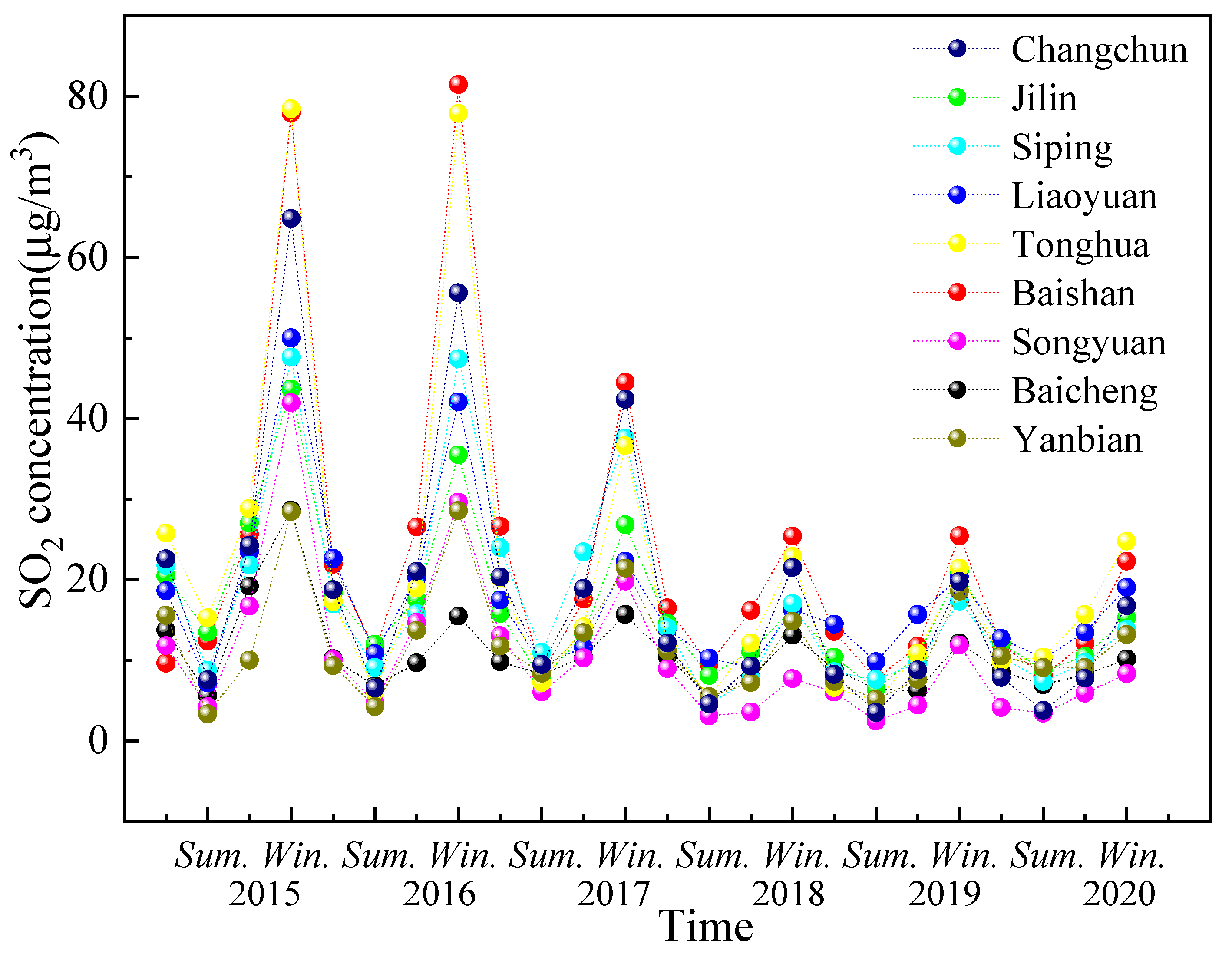
Figure 4 shows the seasonal variation of SO2 concentration in different cities. There is a pattern in the seasonal variation of the SO2 concentration across all the cities, where the SO2 concentration values follow the order of winter > autumn > spring > summer. Overall, a decreasing trend with the annual fluctuations was observed, and the variation was the lowest after 2018.
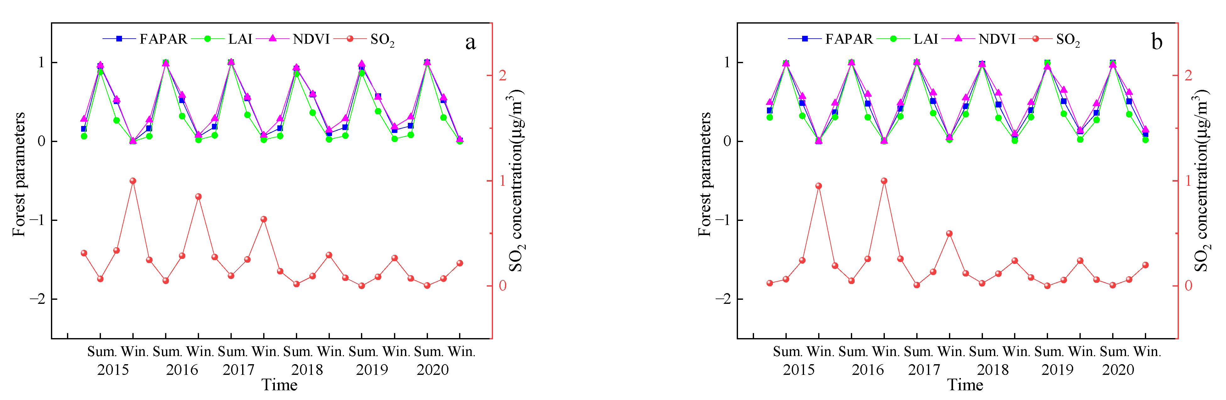
Table 8 shows the relationship between the SO2 concentration and the vegetation parameters across the different seasons from 2015–2020. The results show that there is a significant negative correlation between the SO2 concentration and FPAR, LAI, and NDVI values in each city. This means that the values of the vegetation parameters decreased with an increase in the SO2 concentration. The pattern of SO2 concentration and the vegetation parameters across the different cities and seasons from 2015–2020 remained just about constant. To highlight the comparability among the different indicators, normalization was first performed. Figure 5 shows the trends in the SO2 concentration and vegetation parameters during the different seasons in Changchun and Baishan City from 2015–2020. The results show that there was an opposite trend between SO2 concentration and the vegetation parameters with changes in seasons.
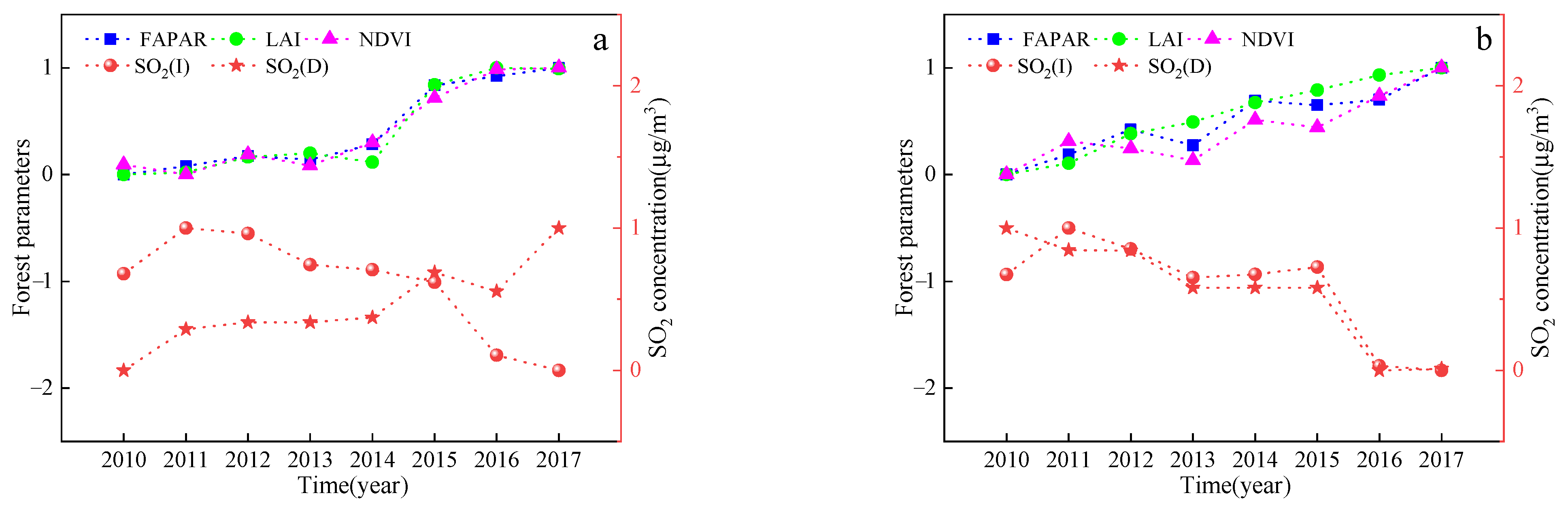
Table 9 shows the relationship between domestic and industrial SO2 emissions and characteristic vegetation values for 2015–2020, from which it can be seen that there was a negative relationship between industrial SO2 emissions and the vegetation parameters in Jilin and Liaoyuan City, where the vegetation parameters decreased as the SO2 concentration increased.
In contrast, there was a significant positive correlation between domestic SO2 emissions and the vegetation parameters in Jilin City, where the values of the vegetation parameters increased with increasing SO2 concentrations, which may play a contributing role. Figure 6 shows the trends of domestic and industrial SO2 emissions and vegetation characteristics for 2015–2020 in Jilin and Liaoyuan cities. With the exception of domestic SO2 emissions in Jilin, there is an opposite trend between SO2 emissions and the annual FPAR, LAI, and NDVI values. The decrease in FPAR, LAI, and NDVI with increasing SO2 emissions shows that industrial SO2 emissions have a greater impact on vegetation than do domestic emissions.
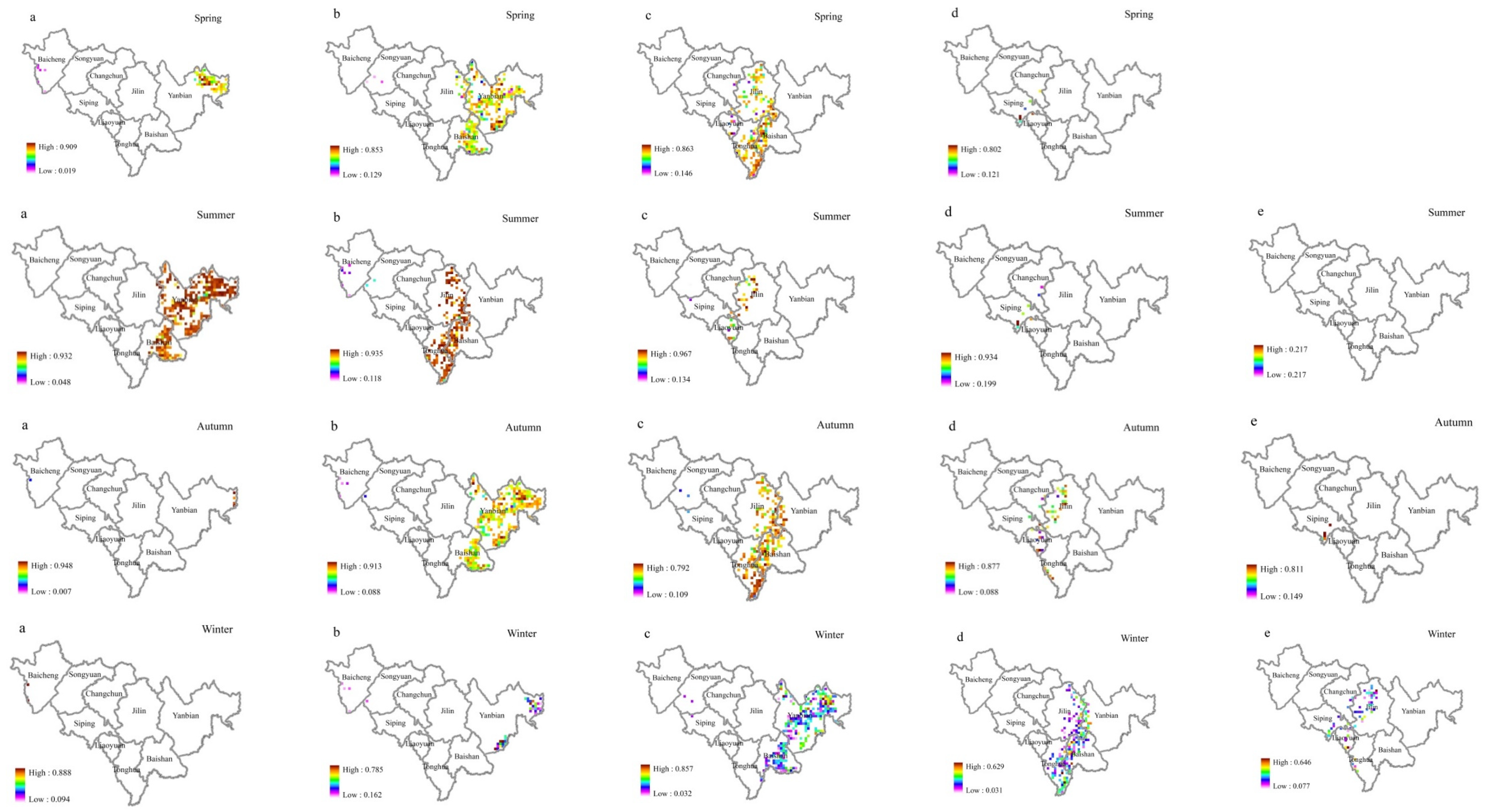
In order to distinguish the seasonal effect and the impact of ρ(SO2) in the air on vegetation, the distribution of correlation coefficient between different ρ(SO2) and GPP in the same season from 2015 to 2020 is discussed (Figure 7). It can be seen that there is a negative spatial correlation between GPP and ρ(SO2) in most regions. In summer, in the middle-east region with a high forest land density in Jilin Province, the central Jilin and Tonghua with high concentrations tend to be more negatively correlated, while the eastern Yanbian with a low concentration tends to be more positively correlated.
4. Discussion
As an important physiological indicator of plants, variations in chlorophyll SPAD, leaf temperature, green-peak and red-valley reflectance, and Fv/Fm are closely related to changes in stomatal aperture, leaf water content, photosynthetic activity, and enzyme activity [49,53]. As plants are exposed to SO2, photosynthesis is inhibited and chlorophyll is converted to demagnetized chlorophyll [54]. The limitation of photosynthesis can be divided into stomatal and non-stomatal factors [55,56], with the stomatal factor showing a decrease in Gs (stomatal conductance) and insufficient CO2 supply and the non-stomatal factor, demonstrating a reduction in the activity of key enzymes for photosynthesis. If Pn decreases along with Gs and Ci, stomatal factors are likely responsible, and if Pn decreases as Ci increases, the main limiting factors for photosynthesis seem to be non-stomatal factors. The chlorophyll content, leaf temperature, green-peak reflectance, and Fv/Fm at 10 days were significantly lower than those at 40 days, regardless of the sampling date or SO2 concentration. The SO2 resistance for the 10-day leaves was consistently lower than for the 40-day leaves.
Juveniles of most plants are more sensitive to environmental changes and extremes, even in resilient species. This is because they require a more suitable environment to re-establish a fully independent SPAC system from a dormant state that is isolated from the soil and atmosphere. Some plants are salt-tolerant to the point of being salt-loving, and moderate salinity is beneficial to their growth [18]. However, the seed germination of these plants is sensitive to salt, and rainfall and other salinity-eluting environments are more conducive to seed germination. The fragile tissue structure and low lignification of seedlings of some tree species makes them vulnerable to adverse effects, such as extreme low temperatures and summer droughts.
The stomatal opening of red-leaved P. cerasifera was the largest and the least vulnerable to SO2 damage. Omasa [57] also found that the stomata of the lightly damaged parts of leaves were more open during the examination of the damage caused by SO2 on plants. This study also concluded that red leaves of P. cerasifera were slightly damaged, followed by S. oblate with green leaves, while U. pumila with yellow leaves were the most damaged. Significant differences in the stomatal aperture values were also observed. Red-leaved tree species with large stomatal aperture values have a stable metabolic balance of water and energy, excellent growth conditions, resistance to adversity, and ability to resist atmospheric pollution.
4.1. Effect of SO2 Stress on Vegetation Characteristics
SO2 concentrations in summer, spring (autumn), and winter were differently regarded as T1, T2, and T3, respectively. As the SO2 treatment concentration increased, the values of the vegetation parameters first increased and then decreased. That is, the highest SO2 concentration and the lowest values for the vegetation parameters were observed in the winter, the lowest SO2 concentration and the highest FPAR, LAI, and NDVI values were observed in the summer, and the SO2 concentration and FPAR, LAI, and NDVI values were in the middle of summer and winter in spring and autumn. The SO2 concentration in autumn is higher than that in spring, and the values of the vegetation parameters are also higher, which may be related to the vegetation characteristics during the growing season. These coincide with the results previously obtained from this study. The results in Table 3 and Table 5 suggest that a medium dose (T2) of SO2 had a positive effect on the studied trees; the reduction in SO2 concentration resulted in an increased reduction in SO2 emissions. This resulted in an increased frequency of S deficiency in the crops and thus increased S fertilization. It is clear that excessive emissions of SO2 (T3) result in the destruction of pine forests and acid rain, but the complete reduction of these emissions has certain disadvantages [58].
4.2. Broadleaf Tree Resistance to SO2 Stress in Different Seasons
According to results of laboratory study, the 10-day leaf resistance performance of the three tree species under different SO2 stress concentrations was as follows: P. cerasifera > S. oblate > U. pumila, on 9 September. As leaf age increased, chlorophyll content and the net photosynthetic rate of the leaf gradually increased, which is closely related to the physiological changes that occur in the leaf during development [59]. Different leaf growth conditions lead to differences in leaf pigment, moisture content, nitrogen, phosphorus, potassium, and other trace elements, as well as differences in cell structure and function. These changes affect the absorption and reflection of light, and ultimately lead to greater differences in the internal chemical composition and tolerance at different locations on the same leaf [60,61,62,63]. In addition to the phenological variations between the upper and lower plant parts, phenological differences between leaves in sun and those in shade have also been found in the canopy or branches [13,64,65].
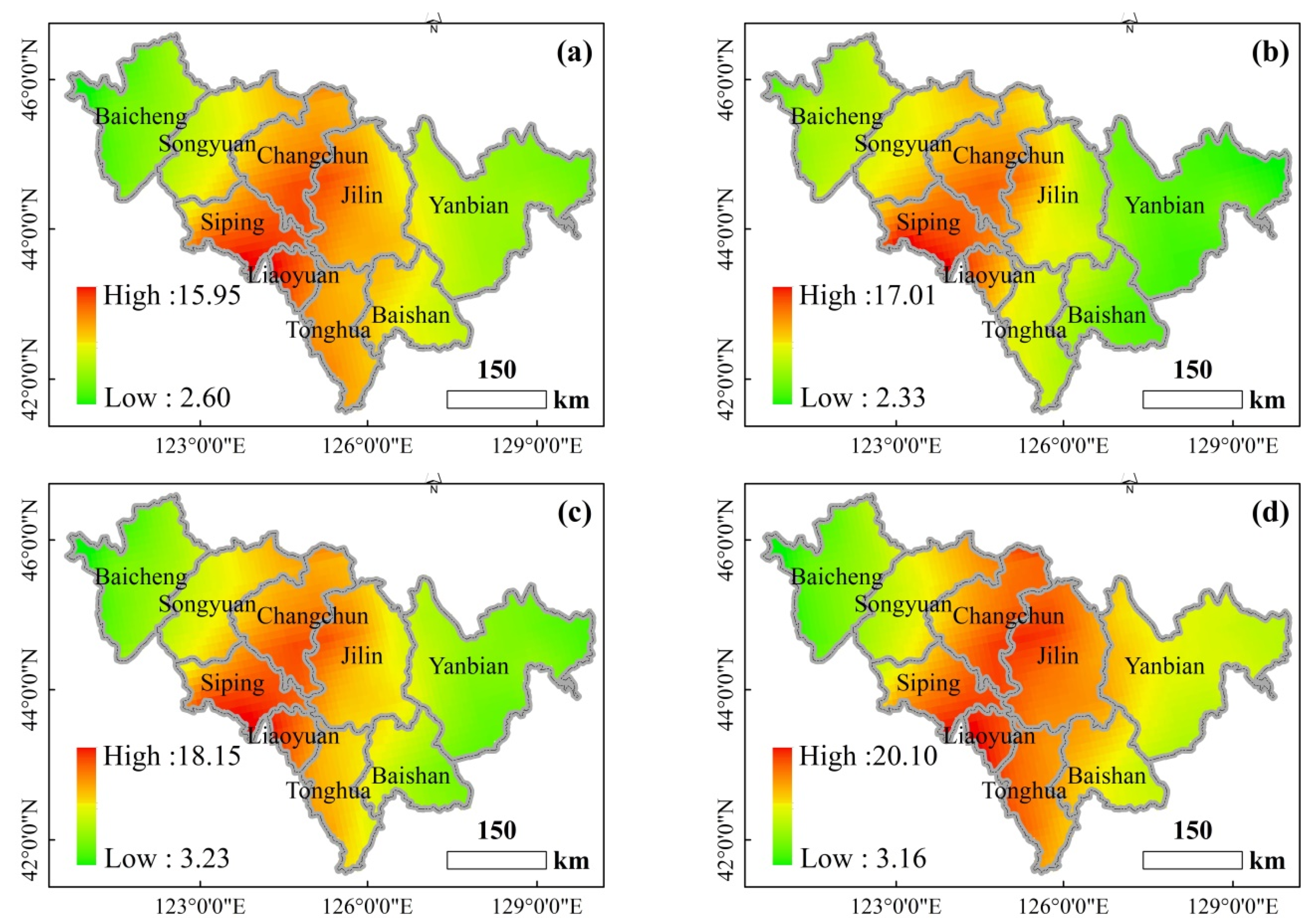
The resistance of different plants to SO2 is known to vary significantly [18]. In general, herbaceous plants are more sensitive than woody plants, coniferous trees are more sensitive than broad-leaved trees, and deciduous broad-leaved trees are more sensitive than evergreen trees. In addition, previous studies have investigated the resistance and purification ability of evergreen and deciduous plants [66,67,68]. In this study, broadleaf trees differed in their resistance to different concentrations of SO2. Figure 8 shows broadleaf tree resistance to SO2 stress during different seasons. Resistance decreased with increasing ρ(SO2) class in different seasons. In the same ρ(SO2) class, the resistance in different seasons was in the following order: summer > autumn > spring > winter. The resistance of different tree species to SO2 is affected by season. In this study, the order of ρ(SO2) in different seasons was winter > autumn > summer > spring; however, the difference was not significant (Figure 9). When SO2 is absorbed by a plant leaf, it can form sulfites, which are then oxidized to sulfates and turned into nutrients useful for plant growth. As the leaves age and wither, they can then continuously transfer sulfur dioxide from the air to the soil, creating a cycle that allows the air to be continuously purified [69]. The leaves renew in the spring, which results in a reduction in sulfur dioxide emissions in the spring. Notably, although the amount of FP (fine particle) collected by vegetation is affected by the season [18], the current study has determined that the seasonal differences was not statistically significant. One study conducted in a high-traffic area in Nanjing, China, showed that the order of different seasons in which dust was retained by trees could be ranked as winter > autumn > summer > spring [70]. Another study conducted in Qingdao, China, reported that the dust retention capacity of ground cover plants showed seasonal variation in the order of winter > spring > autumn > summer [18]. This may be due to the dry winter climate, a greater FP content in the air, and a lesser effect of rainfall. In the summer rainfall, a high relative humidity of the air, a lesser FP content in the air, and SO2 pollution is also the same. Song et al. [71] found that the season with the highest concentration of PM 2.5 in 2013 was winter (112.30 mg/m3), while the cleanest season was summer (44.63 mg/m3).
4.3. Correlation between GPP and ρ(SO2) in Different Vegetation Types
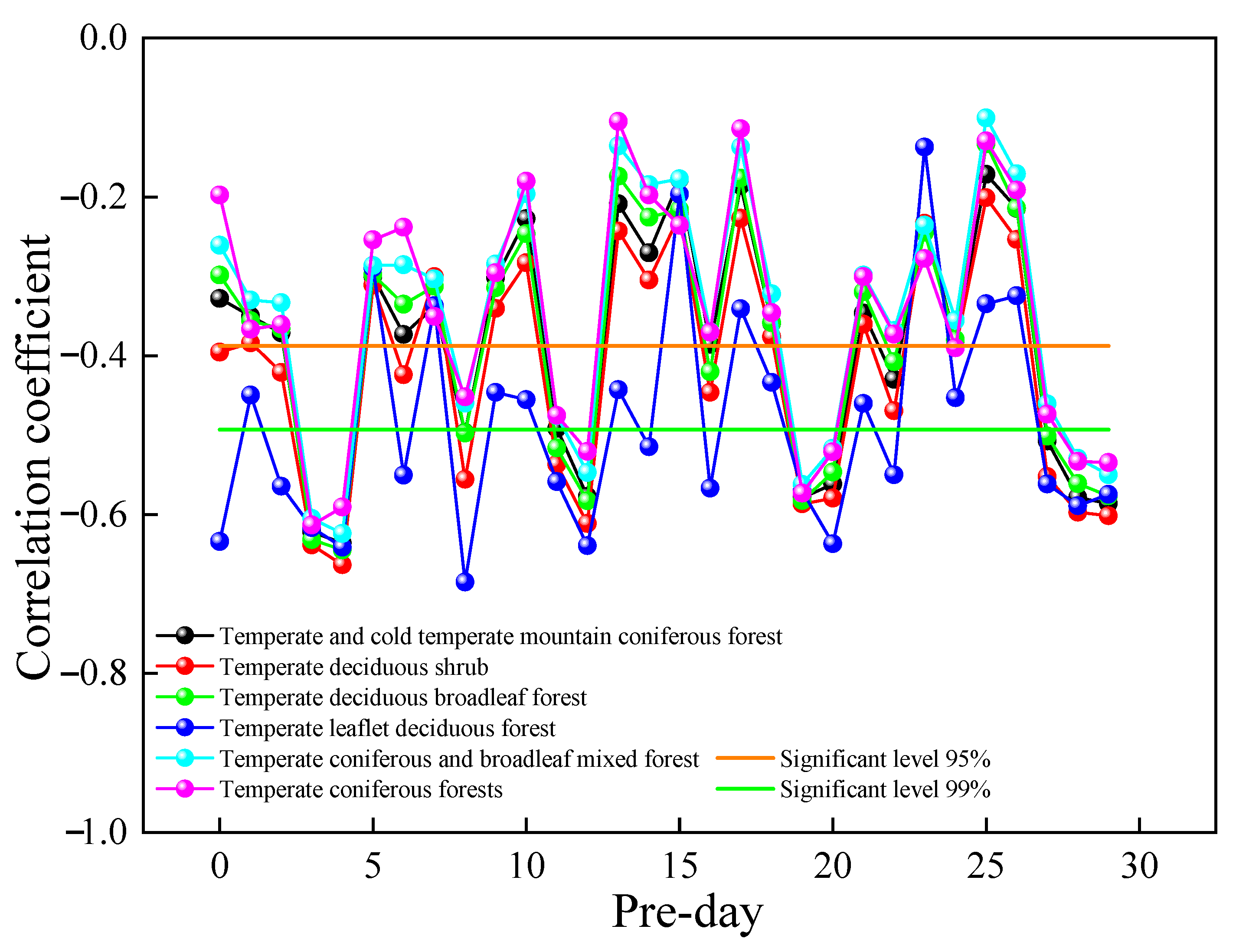
The resistance and resilience of deciduous broad-leaf forest and rational needleleaf forests differ under different continuous drought events [72]. Changes in vegetation GPP can be affected by the concentration of air pollutants. Therefore, by analyzing the relationship between GPP and SO2 concentration at the time corresponding to the experiment, we can better reveal the relationship between GPP changes and SO2 concentrations. In this study, a correlation analysis was performed between the GPP of different vegetation types and their corresponding urban air SO2 concentrations for the previous 30 days. Figure 10 shows a plot of the correlation coefficients between vegetation GPP and urban air SO2 concentrations from that day to the previous 30 days in 2019. The correlation coefficients were found to be more significant with the SO2 concentrations in the previous four days, and the correlations between GPP and SO2 concentrations on other dates were unstable, with highly significant negative correlations with the SO2 concentrations in the previous four days. The relationship between the change in GPP and the change in SO2 concentration from the current day to the previous 30 days was compared to reveal the influence of SO2 concentration on GPP rhythm. From the results, the GPP change was consistent with the SO2 concentration change in the previous four days, indicating a lag in GPP change in SO2 in the previous four days. The correlation between different vegetation types, GPP, and SO2 concentrations in the previous four days could be ranked in the following order: temperate deciduous shrub > temperate deciduous broadleaf forest > temperate leaflet deciduous forest > temperate and cold temperate mountain coniferous forest > temperate coniferous and broadleaf mixed forest > temperate coniferous forests.
The high concentration of SO2 inhibits the growth of vegetation, which can be explained by the effect of SO2 pollution on plants, which is macroscopically manifested as interference with the normal growth and development of vegetation, leading to dwarfing, a smaller leaf area, a lower pollination rate and a lower yield, which results in lower plant GPP. Winter is affected by the seasonal effect, which leads to a more abnormal correlation coefficient. Urban development boundaries and industrial parks mostly showed negative correlations, indicating that human activities have an impact on urban green tree growth. Some study areas, including primary forests in the northeast and low vegetation cover areas in the northwest and south, showed positive correlations because primary forests have a stable vegetation cover [73] and stronger ecological functions, while low vegetation cover areas contain more building sites and lower SO2 concentrations. Based on this, it is difficult for low SO2 concentrations to affect vegetation GPP. The amount of precipitation in an area affects the type and growth state of vegetation, which in turn affects its ability to resist SO2 pollution.
5. Conclusions
The results demonstrated that the chlorophyll content, leaf temperature, green-peak reflectance, and Fv/Fm at 10 days were significantly lower than those at 40 days, regardless of the sampling date or SO2 concentration. Based on this, the resistance of the three green tree species to SO2 at different ontogenies was comprehensively evaluated. The SO2 resistance for the 10-day leaves was consistently lower than that for the 40 days leaves. On 9 September, the 10-day leaf resistance performance of the three tree species under different SO2 stress concentrations was as follows: P. cerasifera > S. oblate > U. pumila. Finally, the spatial products of FPAR, GPP, LAI, and NDVI were combined to explore the resistance mechanisms of broadleaf trees to different SO2 concentration classes during varied seasons on a large scale. Resistance decreased with the increasing ρ(SO2) class in different seasons. The resistance of different tree species to SO2 was affected by season. In addition, the GPP change was consistent with the SO2 concentration change in the previous four days, indicating a lag in GPP change in SO2 in the previous four days. We conclude that mature leaves are more resistant to SO2 stress than young leaves are. The results of this study on changes in the functional traits of urban greening trees and environmental factors, as well as the response of functional traits to environmental changes, will provide a basis for the scientific guidance of artificial plant community construction and the prevention of vegetation degradation in the future.
Author Contributions
All authors contributed meaningfully to this study. A.H.: conceptualization, writing—original draft. Y.B. (Yongbin Bao): investigation, data curation. X.L.: conceptualization, methodology. Z.T.: writing—review and editing. S.Q.: visualization, supervision. Y.B. (Yuhai Bao): conceptualization, resources. J.Z.: conceptualization, writing—review and editing. All authors have read and agreed to the published version of the manuscript.
Funding
This study was financially supported by the National Natural Science Foundation of China (31770770); The International (Regional) cooperation and Exchange Programs of National Natural Science Foundation of China (41961144019); The Major Scientific and Technological Program of Jilin Province (20200503002SF); The Science and Technology Development Planning of Jilin Province (20190303081SF).
Data Availability Statement
Not applicable.
Acknowledgments
The authors are grateful to the anonymous reviewers for their in insightful and helpful comments to improve the manuscript. Furthermore, thanks to Junhui Wang, Bingxin Gui, Yining Ma, Suri Guga, Jie Xu, Mingxi Zhang and Dao Riao of the Disaster Institute group for their help in the field experiments of this study.
Conflicts of Interest
The authors declare no conflict of interest.
References
- Tagil, S.; Tecer, L.; Hakan. Impact of urbanization on local air quality: Differences in urban and rural areas of balikesir, turkey. Clean-Soil Air Water 2014, 42, 1489–1499. [Google Scholar] [CrossRef]
- Ge, W.; Liu, J.; Yi, K.; Xu, J.; Zhang, Y.; Hu, X.; Ma, J.; Wang, X.; Wan, Y.; Hu, J.; et al. Influence of atmospheric in-cloud aqueous-phase chemistry on global simu-lation of SO2 in CESM2. Atmos. Chem. Phys. 2021, 6, 406. [Google Scholar] [CrossRef]
- Yan, X.; Shi, W.; Zhao, W.; Luo, N. Estimation of atmospheric dust deposition on plant leaves based on spectral features. Spectrosc. Lett. 2014, 47, 536–542. [Google Scholar] [CrossRef]
- Jim, C.Y.; Chen, W.Y. Assessing the ecosystem service of air pollutant removal by urban trees in Guangzhou (China). J. Environ. Manag. 2007, 88, 665–676. [Google Scholar] [CrossRef]
- Paull, N.J.; Krix, D.; Irga, P.J.; Torpy, F.R. Green wall plant tolerance to ambient urban air pollution. Urban For. Urban Gree. 2021, 63, 127201. [Google Scholar] [CrossRef]
- Ekene, N.K.; Chigozie, I.B.; Evelyn, U.O.; Nwakaego, E.E.; Ifeoma, O.J. Sensitivity and tolerance index of selected plant species as bioindicators of air pollution stress in abakaliki, ebonyi state, nigeria. Middle East J. Sci. Res. 2019, 27, 144–152. [Google Scholar] [CrossRef]
- Singh, S.K.; Rao, D.N.; Agrawal, M.; Pandey, J.; Naryan, D. Air pollution tolerance index of plants. J. Environ. Manag. 1991, 32, 45–55. [Google Scholar] [CrossRef]
- Gao, Q.; Yu, M. Canopy density and roughness differentiate resistance of a tropical dry forest to major hurricane damage. Remote Sens. 2021, 13, 2262. [Google Scholar] [CrossRef]
- Majernik, O.; Mansfield, T.A. Effects of SO2 pollution on stomatal movements in Vicia faba. J. Phytopathol. 1971, 71, 0123–0128. [Google Scholar] [CrossRef]
- Katainen, H.S.; Mäkinen, E.; Jokinen, J.; Karjalainen, R.; Kellomaki, S. Effects of SO2 on the photosynthetic and respiration rates in Scots pine seedlings. Environ. Pollut. 1987, 46, 241–251. [Google Scholar] [CrossRef]
- Baxter, R.; Emes, M.J.; Lee, J.A. Effects of the bisulphite ion on growth and photosynthesis In Sphagnum cuspidatum Hoffm. New Phytol. 1989, 111, 457–462. [Google Scholar] [CrossRef] [PubMed]
- Katiyar, V.; Dubey, P.S. Amelioration of SO2 stress under fertilizer regime in a vegetable crop. Int. J. Environ. Stud. 2005, 62, 95–99. [Google Scholar] [CrossRef]
- Muneer, S.; Kim, T.H.; Choi, B.C.; Lee, B.S.; Lee, J.H. Effect of CO, NOx and SO2 on ROS production, photosynthesis and ascorbate-glutathione pathway to induce Fragaria×annasa as a hyperaccumulator. Redox Biol. 2014, 2, 91–98. [Google Scholar] [CrossRef] [PubMed] [Green Version]
- Wei, A.L.; Han, E.Q.; Zhang, X.B.; Wu, F.J.; Xin, X.J.; Wang, T.; Zhang, S.S.; Wang, Y.S.; Cao, D.M. SO2-induced stomatal movement and its signal regulation in guard cells of Hemerocallis fulva. J. Environ. Sci. 2016, 36, 740–746. [Google Scholar] [CrossRef]
- Callahan, D.L.; Hare, D.J.; Bishop, D.P.; Doble, P.A.; Roessner, U. Elemental imaging of leaves from the metal hyperaccumulating plant noccaea caerulescens shows different spatial distribution of Ni, Zn and Cd. RSC Adv. 2016, 6, 2337–2344. [Google Scholar] [CrossRef] [Green Version]
- Deljanin, I.; Antanasijević, D.; Bjelajac, A.; Urošević, M.A.; Ristić, M. Chemometrics in biomonitoring: Distribution and correlation of trace elements in tree leaves. Sci. Total Environ. 2016, 545, 361–371. [Google Scholar] [CrossRef] [PubMed]
- Chen, S.; Oliva, P.; Zhang, P. The Effect of Air Pollution on Migration: Evidence from China; National Bureau of Economic Research: Cambridge, MA, USA, 2017. [Google Scholar] [CrossRef]
- Zhang, Z.; Liu, J.; Wu, Y.; Yan, G.; Zhu, L.; Yu, X. Multi-scale comparison of the fine particle removal capacity of urban forests and wetlands. Sci. Rep-UK 2017, 7, 46214. [Google Scholar] [CrossRef] [Green Version]
- Zhang, J.; Li, J.; Jiang, J. A Study on Water Parameters of Plantations in Mountain Areas of West Beijing (Ⅲ). J. Beijing For. Univ. 1994, 16, 46–53. [Google Scholar]
- Yang, M.; Pei, B.; Zhang, S. Advances in drought resistance of trees. Hebei J. For. Orchard R. 1997, 12, 87–93. [Google Scholar]
- Sun, Z.H. A study on the Drought Resistance of Acer Ginnala, Malus Baccata, Prunus Davidiana and Pyrus Ussuriensis. Doctoral Dissertation, Northeast Forestry University, Harbin, China, 2002. [Google Scholar]
- Steimetz, E.; Trouvelot, S.; Gindro, K.; Bordier, A.; Poinssot, B.; Adrian, M.; Daire, X. Influence of leaf age on induced resistance in grapevine against plasmopara viticola. Physiol. Mol. Plant P. 2012, 79, 89–96. [Google Scholar] [CrossRef]
- Develey-Riviere, M.P.; Galiana, E. Resistance to pathogens and host developmental stage: A multifaceted relationship within the plant kingdom. New Phytol. 2007, 175, 405–416. [Google Scholar] [CrossRef] [PubMed]
- Farber, D.H.; Mundt, C.C. Effect of plant age and leaf position on susceptibility to wheat stripe rust. Phytopathology 2017, 107, 412–417. [Google Scholar] [CrossRef] [PubMed]
- Mediavilla, S.; González-Zurdo, P.; García-Ciudad, A.; Escudero, A. Morphological and chemical leaf composition of mediterranean evergreen tree species according to leaf age. Trees 2011, 25, 669–677. [Google Scholar] [CrossRef]
- Mediavilla, A.E. Decline in photosynthetic nitrogen use efficiency with leaf age and nitrogen resorption as determinants of leaf life span. J. Ecol. 2003, 91, 880–889. [Google Scholar] [CrossRef]
- Gilmore, D.W.; Seymour, R.S.; Halteman, W.A.; Greenwood, M.S. Canopy dynamics and the morphological development of abies balsamea: Effects of foliage age on specific leaf area and secondary vascular development. Tree Physiol. 1995, 15, 47. [Google Scholar] [CrossRef] [PubMed] [Green Version]
- Kuuluvainen, T.; Gauthier, S. Young and old forest in the boreal:critical stages of ecosystem dynamics and management under global change. For. Ecosys. 2018, 5, 5–26. [Google Scholar] [CrossRef]
- Adler, P.B.; Salguero-Gómez, R.; Compagnoni, A.; Hsu, J.S.; Ray-Mukherjee, J.; Mbeau-Ache, C.; Franco, M. Functional traits explain variation in plant life history strategies. Proc. Natl. Acad. Sci. USA 2014, 111, 740–745. [Google Scholar] [CrossRef] [PubMed] [Green Version]
- Chen, Z.; Zhang, Y.; Yuan, W.; Zhu, S.D.; Liu, S.; Wan, X.C.; Liu, S.R. Coordinated variation in stem and leaf functional traits of temperate broadleaf tree species in the isohydric-anisohydric spectrum. Tree Physiol. 2021, 41, 1601–1610. [Google Scholar] [CrossRef]
- Diaz, S.; Fraser, L.H.; Grime, J.P.; Falczuk, V. The impact of elevated co2 on plant-herbivore interactions: Experimental evidence of moderating effects at the community level. Oecologia 1998, 117, 177–186. [Google Scholar] [CrossRef]
- Omasa, K.; Hashimoto, Y.; Aiga, I. A Quantitative analysis of the relationships between SO2 or N02 sorption and their acute effects on plant leaves using image instrument. Environ. Control. Biol. 1981, 19, 59–67. [Google Scholar] [CrossRef]
- Nilsson, H.E. Remote-sensing and image-analysis in plant pathology. Can. J. Plant Pathol. 1995, 17, 154–166. [Google Scholar] [CrossRef]
- Kooistra, L.; Wehrens, R.; Leuven, R.S.E.W.; Buydens, L.M.C. Possibilities of visible-near-infrared spectroscopy for the assessment of soil contamination in river flood plains. Anal. Chim. Acta 2001, 446, 97–105. [Google Scholar] [CrossRef]
- Rossel, R.A.V.; Walvoort, D.J.J.; Mcbratney, A.B.; Janik, L.J.; Skjemstad, J.O. Visible, near infrared, mid infrared or combined diffuse reflectance spectroscopy for simultaneous assessment of various soil properties. Geoderma 2006, 131, 59–75. [Google Scholar] [CrossRef]
- Orwell, R.L.; Wood, R.A.; Burchett, M.D.; Tarran, J.; Torpy, F. The potted-plant microcosm substantially reduces indoor air voc pollution: Ii. laboratory study. Water Air Soil Poll. 2006, 177, 59–80. [Google Scholar] [CrossRef]
- Li, J.; Zhou, G.; Zhang, L.; Li, K. Physiological Responses of Taxus cuspidate to Sulfur Dioxide Stress. Nor. Horticul. 2011, 9, 74–76. [Google Scholar]
- Wang, F.; Wu, D.J.; Zhai, G.; Zang, L. Diagnosing Low Health and Wood Borer Attacked Trees of Chinese Arborvitae by Using Thermograpy. Spectrosc. Spectr. Anal. 2015, 35, 130–135. [Google Scholar]
- Zhao, L.; Jing, J.; Wang, S. Studies on water transports in the soil-plant-atmosphere continuum on WeiBei rainfed highland, Shaanxi procinve—I. Effects of ecological and physiological factors on plant leaf water potential. Acta Bot. Boreal. Occident. Sin. 1996, 16, 345–350. [Google Scholar]
- Cai, H.; Kang, S. The Changing Pattern of Cotton Crop Canopy Tmperature and its Application in Detecing Crop Water Stress. Guangai Paishui. 1997, 16, 1–5. [Google Scholar]
- Anderson, J.M. Photoregulation of the Composition, Function, and Structure of Thylakoid Membranes. Annu. Rev. Plant. Phys. 1986, 37, 93–136. [Google Scholar] [CrossRef]
- Baker, N.R. A possible role for photosystem ii in environmental perturbations of photosynthesis. Phys. Plant. 1991, 81, 563–570. [Google Scholar] [CrossRef]
- Chen, T.; Chang, Q.; Clevers, J.G.; Kooistra, L. Rapid identification of soil cadmium pollution risk at regional scale based on visible and near-infrared spectroscopy. Environ. Pollut. 2015, 206, 217–226. [Google Scholar] [CrossRef] [PubMed]
- Li, Y. Resistance to sulfur dioxide of four colored-leaf species in prunus. Sci. Silvae Sin. 2008, 44, 28–33. [Google Scholar]
- Randles, C.A.; Da Silva, A.M.; Buchard, V.; Colarco, P.R.; Darmenov, A.; Govindaraju, R.; Alexander, S.; Holben, B.; Ferrare, R.A.; Hair, J.; et al. The MERRA-2 aerosol reanalysis, 1980 onward. Part I: System description and data assimilation evaluation. J. Clim. 2017, 30, 6823–6850. [Google Scholar] [CrossRef] [PubMed]
- Buchard, V.; Randles, C.A.; Da Silva, A.M.; Darmenov, A.; Colarco, P.R.; Govindaraju, R.; Ferrare, R.; Hair, J.; Beyersdorf, A.J.; Ziemba, L.D.; et al. The MERRA-2 aerosol reanalysis, 1980 onward. Part II: Evaluation and case studies. J. Clim. 2017, 30, 6851–6872. [Google Scholar] [CrossRef]
- Gelaro, R.; McCarty, W.; Suárez, M.J.; Todling, R.; Molod, A.; Takacs, L.; Wargan, K. The modern-era retrospective analysis for research and applications, version 2 (MERRA-2). J. Clim. 2017, 30, 5419–5454. [Google Scholar] [CrossRef] [PubMed]
- Eltahan, M.; Magooda, M. Spatiotemporal Assessment of SO2, SO4 and AOD From Over MENA Domain From 2006 to 2016 Using Multiple Satellite Data and Reanalysis MERRA2 Data. J. Geosci. Environ. Prot. 2018, 7, 156–174. [Google Scholar] [CrossRef] [Green Version]
- Wu, C.; Munger, J.W.; Niu, Z.; Kuang, D. Comparison of multiple models for estimating gross primary production using MODIS and eddy co-variance data in Harvard Forest. Remote Sens. Environ. 2010, 114, 2925–2939. [Google Scholar] [CrossRef]
- Xiao, J.; Zhuang, Q.; Law, B.E. A continuous measure of gross primary production for the conterminous United States derived from MODIS and AmeriFlux data. Remote Sens. Environ. 2010, 114, 576–591. [Google Scholar] [CrossRef] [Green Version]
- Wu, Z. The Research of the Vegetation Change and the Sensitivity between NDVI and Climatic Factors in Qilian Mountains from 2000 to 2012. Master’s Thesis, Northwest Normal University, Changchun, China, 2014. [Google Scholar] [CrossRef]
- Wu, Z.; Tan, X.; Yuan, J.; Huang, L. Morphology and photosynthetic parameters of Camellia oleifera leaves at different ages. Nonwood For. Res. 2016, 34, 6. [Google Scholar]
- Wang, H.; Wang, J.; Hu, Y.; Guo, H. Relationship between Flue_cured Tobacco Maturity and Leaf Angle. Tobacco Sci. Technol. 2005, 8, 32–34. [Google Scholar]
- Li, D.; Zhang, S.; Xu, Z. Relationship between Main Chemical Components in Leaf and Leaf Length in Different Positions in Tobacco (Nicotiana tabacum L.). Acta Agron. Sin. 2008, 34, 914–918. [Google Scholar] [CrossRef]
- Xu, A.; Xie, H.; Dai, X.; Yang, C.; Wang, Y.; Chen, W.; Liu, H.; Ye, X. Effects of Ridge-direction on Photosynthetic Characteristics of Leaves in Different Positions in Flue-cured Tobacco Field. Acta Agric. Jiangxi 2011, 23, 136–138. [Google Scholar]
- Wang, T.; He, F.; Zhan, J.; Huo, K.; Zhao, H.; Wang, M.; Gong, C. Color parameters and chemical components in different leaf positions of flue-cured tobacco leaves during bulk curing process. J. Hunan Agric. Univ. 2012, 38, 125–130. [Google Scholar] [CrossRef]
- Liu, Q. Study on Injury Response and Biochemical Resistantance to SO2 of Plants. Doctoral Dissertation, Shanxi Agricultural University, Jinzhong, China, 2003. [Google Scholar]
- Shu, J.; Cao, H.; Liu, Y.; Gao, Y. Effects of long-term exposure of Low concentration SO2 on the growth and Yield of Soybean. J. Ecojogy. 1990, 9, 28–30. [Google Scholar] [CrossRef]
- Liu, Q. Study on Acute Injury Symptom to SO2 of plant. Chin. Hort. Abs. 2009, 25, 15–16, 54. [Google Scholar]
- Omasa, K.; Saji, H. Air Pollution and Plant Biotechnology: Prospects for Phytomonitoring and Phytoremediation; Springer: Tokyo, Japan, 2002. [Google Scholar] [CrossRef]
- Zhou, N.; Jing, L.Q.; Wang, Y.X.; Zhu, J.G.; Yang, L.X.; Wang, Y.L. Dynamic effects of CO2 concentration and temperature increase on chlorophyll content and SPAD value in rice leaves in open air. Chin. Rice Sci. 2017, 31, 524–532. [Google Scholar]
- Mclaughlin, S.B.; Mcconathy, R.K. Effects of so2 and o3 on allocation of 14c-labeled photosynthate in phaseolus vulgaris. Plant Physiol. 1983, 73, 630–635. [Google Scholar] [CrossRef] [Green Version]
- Van Heerden, P.D.R.; Strasser, R.J.; Krüger, G.H.J. Reduction of dark chilling stress in N2-fixing soybean by nitrate as indicated by chlorophyll a fluorescence kinetics. Physiol. Plantarum. 2004, 121, 239–249. [Google Scholar] [CrossRef]
- Shi, K.; Ze, L.I.; Zhang, W.; Xiao, H.E.; Zeng, Y.; Tan, X. Influence of different light intensity on the growth, diurnal change of photosynthesis and chlorophyll fluorescence of tung tree seedling. J. Central South Univ. For. Technol. 2018, 38, 35–42. [Google Scholar]
- Wang, F.; Zhang, J.Q. Important Characteristics and Mechanisms of Woody Plants in Response to Environmental Stress; Science Press: Beijing, China, 2017. [Google Scholar]
- Chen, Z.; Du, G.; Miao, Y. Resistance to and absorption of gaseous HF with 38 landscaping plant species in Zhejiang Province. J. Zhejiang For. Coll. 2008, 25, 475–480. [Google Scholar] [CrossRef]
- Miao, Y.; Chen, Z.; Chen, Y.; Du, G. Resistance to and absorbency of gaseous NO2 for 38 young landscaping plants in Zhejiang Province. J. Zhejiang For. Coll. 2009, 25, 765–771. [Google Scholar] [CrossRef]
- Sun, F.B.; Yin, Z.; Lun, X.; Zhao, Y.; Li, R.; Shi, F.; Yu, X. Deposition Velocity of PM2.5 in the Winter and Spring above Deciduous and Coniferous Forests in Beijing, China. PLoS ONE 2014, 9, e97723. [Google Scholar] [CrossRef]
- Lu, M.; Li, Y. Research on absorption and purgation ability to atmospheric pollutants of some garden plants. J. Shandong Ins. Arch. Eng. 2002, 17, 45–49. [Google Scholar] [CrossRef]
- Wang, K.; Hai-Mei, L.I. Effect of Dust-detaining of Ground Cover Plants in Chengyang District of Qingdao City. Acta Agric. Jiangxi 2009, 21, 68–70. [Google Scholar]
- Song, Y.S.; Wang, X.K.; Maher, B.A.; Li, F.; Xu, C.; Liu, X.; Sun, X.; Zhang, Z. The spatial-temporal characteristics and health impacts of ambient fine particulate matter in china. J. Clean Prod. 2016, 112, 1312–1318. [Google Scholar] [CrossRef]
- Liu, M. Forest resistance and resilience to 2002 drought in northern china. Remote Sens. 2021, 13, 2919. [Google Scholar] [CrossRef]
- Lin, N. Study on the Change and Drving Force of Vegetation Cover in Eastern Jilin Province Based on RS and GIS Technology. Doctoral Dissertation, Jilin University, Changchun, China, 2010. [Google Scholar] [CrossRef]
Figure 1.
Mean leaf spectral reflectance for three different SO2 treatments (T1–T3) on 1 September, 9 September, and 19 September 2019 for S. oblate (a,b), P. cerasifera (c,d) and U. pumila (e,f). Bars sharing a common letter are not significantly different (p < 0.05). Bars represent means ± SE (n = 9). Figure parts (a,c,e) represent the upper 10 days old leaves, and (b,d,f) are the lower 40 days old leaves.
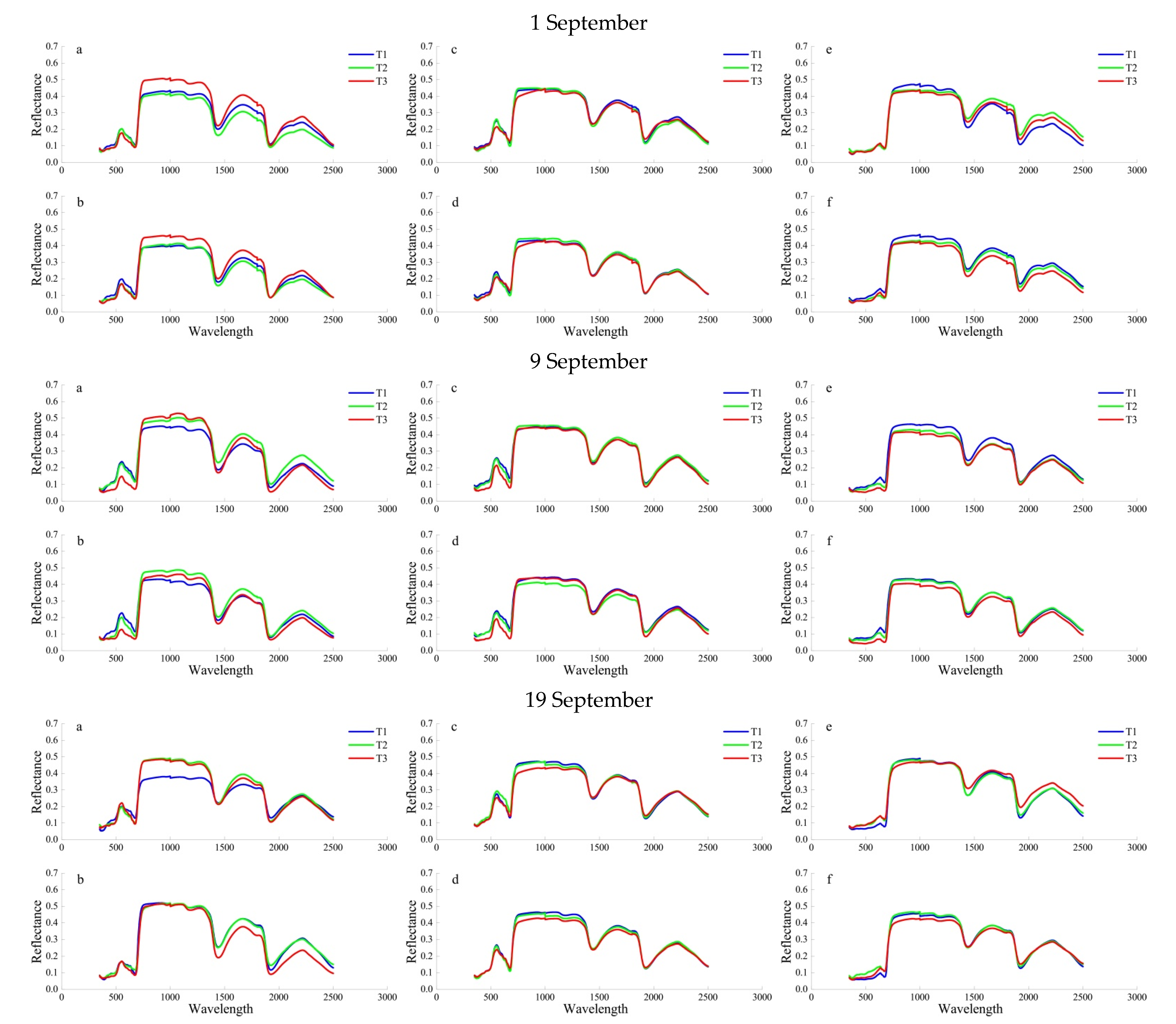
Figure 2.
Light response curves under SO2 stress (9 Sept). (a) Intercellular CO2 concentration, Ci; (b) stomatal conductance, Gs; (c) net photosynthetic rate, Pn and (d) transpiration rate, Tr.
Figure 2.
Light response curves under SO2 stress (9 Sept). (a) Intercellular CO2 concentration, Ci; (b) stomatal conductance, Gs; (c) net photosynthetic rate, Pn and (d) transpiration rate, Tr.
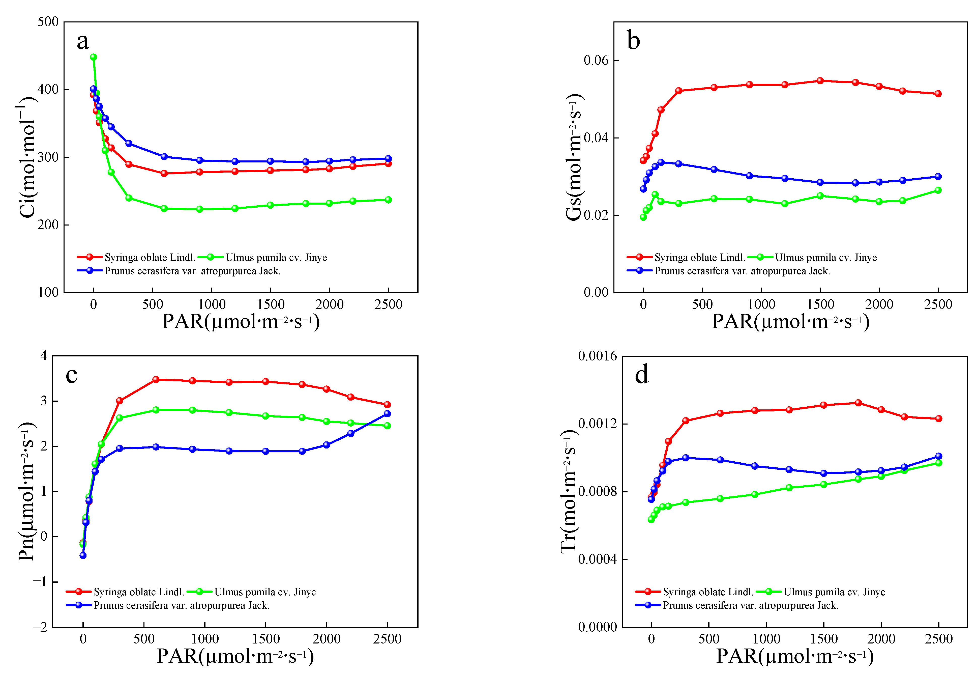
Figure 3.
SO2 emissions from urban emissions in Jilin Province.
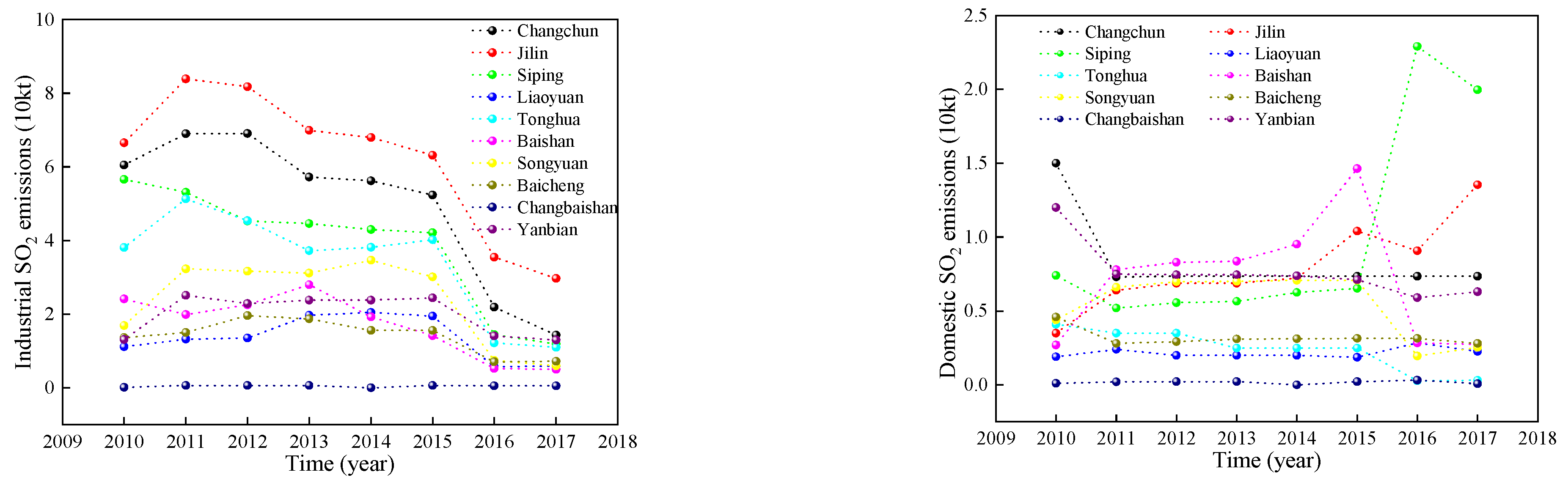
Figure 4.
Variation of SO2 concentration in different seasons from 2015–2020.

Figure 5.
Trends of SO2 concentration and vegetation characteristics in different seasons from 2015–2020 ((a). Changchun, (b). Baishan).
Figure 5.
Trends of SO2 concentration and vegetation characteristics in different seasons from 2015–2020 ((a). Changchun, (b). Baishan).

Figure 6.
Trends in domestic and industrial SO2 emissions and vegetation characteristics in 2015–2020 ((a). Jilin, (b). Liaoyuan).
Figure 6.
Trends in domestic and industrial SO2 emissions and vegetation characteristics in 2015–2020 ((a). Jilin, (b). Liaoyuan).

Figure 7.
Spatial distribution of the correlation between GPP and ρ(SO2) in different months in Spring, Summer and Autumn of 2015–2020. ((a). Mar., (b). Apr., (c). May., (d). Jun., (e). Jul., (f). Aug., (g). Sept., (h). Oct., (i). Nov., (j). Dec., (k). Jan., (l). Feb.).
Figure 7.
Spatial distribution of the correlation between GPP and ρ(SO2) in different months in Spring, Summer and Autumn of 2015–2020. ((a). Mar., (b). Apr., (c). May., (d). Jun., (e). Jul., (f). Aug., (g). Sept., (h). Oct., (i). Nov., (j). Dec., (k). Jan., (l). Feb.).
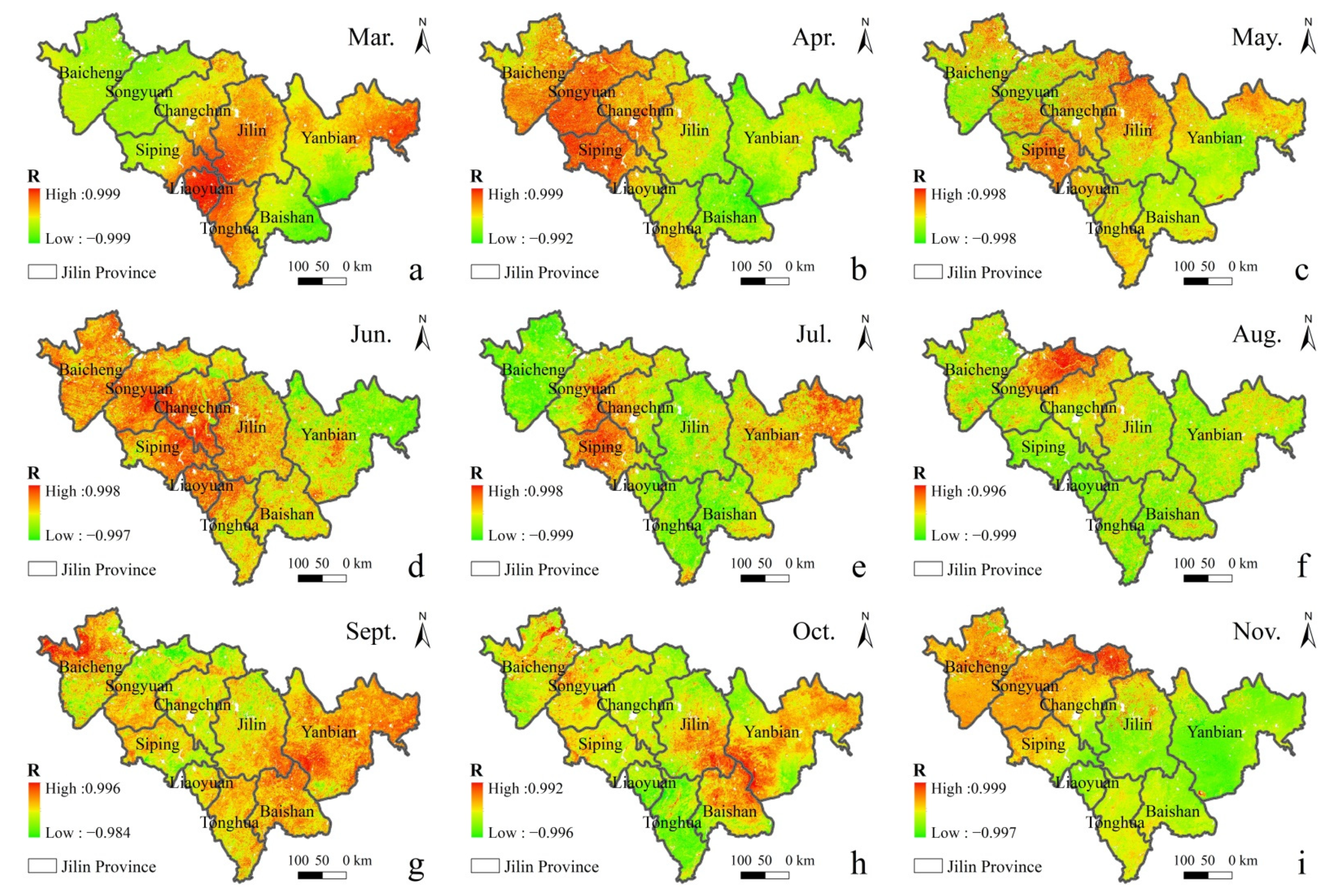
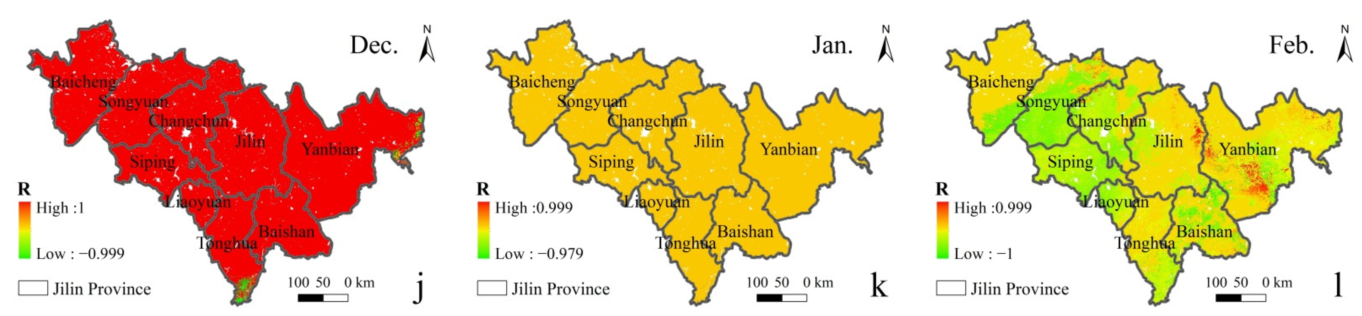
Figure 8.
Broadleaf tree resistance to SO2 stress in different seasons. The figure parts (a–e) represent the ρ(SO2) class. The affiliation values of different ρ(SO2) levels of resistance in the same season ((a). very low, (b). low, (c). moderate, (d). high, (e). very high) are shown horizontally, and the affiliation values of the same ρ(SO2) level of resistance in different seasons are shown vertically.

Figure 9.
The spatial distribution of ρ(SO2) in different seasons in 2015–2020. ((a). Spring, (b). Summer, (c). Autumn, (d). Winter).
Figure 9.
The spatial distribution of ρ(SO2) in different seasons in 2015–2020. ((a). Spring, (b). Summer, (c). Autumn, (d). Winter).

Figure 10.
Relationship between GPP and urban air SO2 concentration for the different vegetation types in 2019.
Figure 10.
Relationship between GPP and urban air SO2 concentration for the different vegetation types in 2019.


Table 1.
Leaf morphology of the three tree species used in this study.
| Time | Tree Species | ||
|---|---|---|---|
| S. oblata | P. cerasifera | U. pumila | |
| Before fumigating | 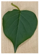 | 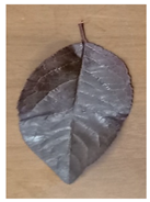 |  |
| After fumigation | 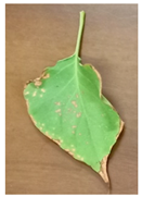 |  |  |
Table 2.
Schedule of SO2 stress experiments in 2019.
| Experiment Time | Experimental Event | |
|---|---|---|
| Before fumigation | 19 May 2019 | Potted plants (1-year-old seedlings) |
| 8 August 2019 | Measure the index before placing in the fumigation chamber | |
| 20–26 August 2019 | Plants placed into the fumigation chamber for 1 week | |
| 28 August 2019 | The indexes were measured after 1 week of adaptation | |
| During fumigation | 30–31 August 2019 | Fumigation |
| 1 September 2019 | Measurement index | |
| 7–8 September 2019 | Fumigation | |
| 9 September 2019 | Measurement index | |
| 13–14 September 2019 | Fumigation | |
| 15 September 2019 | Measurement index | |
| 20–21 September 2019 | Fumigation | |
| 22 September 2019 | Measurement index | |
Table 3.
Leaf chlorophyll SPAD for three different SO2 treatments (T1–T3) on 1 September, 9 September, and 19 September 2019 for S. oblate, P. cerasifera and U. pumila. Bars sharing a common letter are not significantly different (p < 0.05). Bars represent means ± SE (n = 9).
Table 3.
Leaf chlorophyll SPAD for three different SO2 treatments (T1–T3) on 1 September, 9 September, and 19 September 2019 for S. oblate, P. cerasifera and U. pumila. Bars sharing a common letter are not significantly different (p < 0.05). Bars represent means ± SE (n = 9).
| Time | Tree Species | Treatment | 10 Days | 40 Days |
|---|---|---|---|---|
| 1-Sep | S. oblate | T1 | 37.83 ± 5.53 b | 41.63 ± 2.04 b |
| T2 | 48.1 ± 3.05 a | 49.5 ± 2.16 a | ||
| T3 | 20.06 ± 7.08 c | 34.73 ± 6.35 c | ||
| P. cerasifera | T1 | 32.26 ± 0.40 ab | 47.23 ± 2.61 a | |
| T2 | 36.4 ± 1.15 a | 51.9 ± 12.5 a | ||
| T3 | 29.93 ± 0.49 b | 40.96 ± 3.00 a | ||
| U. pumila | T1 | 18.56 ± 1.01 a | 23.1 ± 0.62 b | |
| T2 | 19.23 ± 3.72 a | 29.8 ± 2.95 a | ||
| T3 | 6.9 ± 2.62 b | 18.16 ± 0.66 c | ||
| 9-Sep | S. oblate | T1 | 45.63 ± 1.11 b | 46.8 ± 5.53 ab |
| T2 | 51.2 ± 4.08 a | 54.7 ± 2.49 a | ||
| T3 | 38.6 ± 4.15 c | 42.53 ± 3.80 b | ||
| P. cerasifera | T1 | 33.53 ± 0.46 b | 43.76± b | |
| T2 | 44.4 ± 1.80 a | 55.73 ± 0.51 a | ||
| T3 | 28 ± 1.05 c | 41.4 ± 0.96 c | ||
| U. pumila | T1 | 22.93 ± 2.55 a | 27.63 ± 2.44 a | |
| T2 | 26.73 ± 1.90 a | 28.13 ± 2.10 a | ||
| T3 | 14.56 ± 0.60 b | 24.8 ± 6.21 a | ||
| 19-Sep | S. oblate | T1 | 28.06 ± 2.45 b | 31.76 ± 5.00 ab |
| T2 | 34.13 ± 1.85 a | 39.26 ± 4.74 a | ||
| T3 | 22.26 ± 3.00 c | 20.73 ± 8.50 c | ||
| P. cerasifera | T1 | 27.7 ± 0.26 a | 35.26 ± 4.74 a | |
| T2 | 30.63 ± 2.70 a | 36.76 ± 1.27 a | ||
| T3 | 18.83 ± 2.27 b | 21.5 ± 2.26 b | ||
| U. pumila | T1 | 18.9 ± 2.78 b | 27.13 ± 1.18 b | |
| T2 | 26.26 ± 2.45 a | 36.23 ± 10.8 a | ||
| T3 | 18.53 ± 1.00 b | 19.83 ± 5.84 b |
Table 4.
Leaf temperature for three different SO2 treatments (T1—T3) on 9 September and 19 September 2019 for S. oblate, P. cerasifera and U. pumila. Bars sharing a common letter are not significantly different (p < 0.05). Bars represent means ± SE (n = 9).
Table 4.
Leaf temperature for three different SO2 treatments (T1—T3) on 9 September and 19 September 2019 for S. oblate, P. cerasifera and U. pumila. Bars sharing a common letter are not significantly different (p < 0.05). Bars represent means ± SE (n = 9).
| Time | Tree Species | Treatment | 10 Days | 40 Days |
|---|---|---|---|---|
| S. oblate | T1 | 28.87 ± 0.48 c | 25.39 ± 0.92 c | |
| 9-Sep | T2 | 30.77 ± 0.50 b | 26.99 ± 0.40 b | |
| T3 | 31.77 ± 0.15 a | 28.10 ± 0.42 a | ||
| P. cerasifera | T1 | 29.22 ± 0.80 c | 25.76 ± 0.53 c | |
| T2 | 30.06 ± 0.48 b | 29.10 ± 1.04 b | ||
| T3 | 31.17 ± 1.30 a | 30.44 ± 0.77 a | ||
| U. pumila | T1 | 28.49 ± 2.52 c | 25.92 ± 0.47 c | |
| T2 | 29.31 ± 0.44 b | 28.40 ± 0.48 b | ||
| T3 | 30.35 ± 0.88 a | 30.18 ± 0.18 a | ||
| 19-Sep | S. oblate | T1 | 24.38 ± 0.43 c | 22.22 ± 0.22 c |
| T2 | 29.50 ± 0.81 b | 23.09 ± 0.48 b | ||
| T3 | 30.48 ± 0.46 a | 24.45 ± 0.39 a | ||
| P. cerasifera | T1 | 25.47 ± 0.87 c | 24.15 ± 0.73 c | |
| T2 | 27.43 ± 0.14 b | 25.05 ± 1.35 b | ||
| T3 | 28.79 ± 0.40 a | 26.79 ± 1.00 a | ||
| U. pumila | T1 | 25.36 ± 0.21 c | 22.33 ± 1.92 c | |
| T2 | 26.85 ± 0.77 b | 22.8 ± 0.43 b | ||
| T3 | 27.97 ± 0.74 a | 23.85 ± 1.20 a |
Table 5.
Maximum quantum yield of photosystem II (Fv/Fm) for 10 days old leaves and the lower 40 days old leaves on 1 September, 9 September, and 19 September 2019 for S. oblate, P. cerasifera and U. pumila grown under three different SO2 treatments (T1–T3). Within each treatment and date, statistical differences between 10 days and 40 days (p < 0.05) are denoted with the lower case letters a, b, and c. Data represent means ± SE (n = 9).
| Tree Species | Treatment | 1-Sep | 9-Sep | 19-Sep | |||
|---|---|---|---|---|---|---|---|
| 10 Days | 40 Days | 10 Days | 40 Days | 10 Days | 40 Days | ||
| S. oblata | T1 | 0.61 ± 0.11 b | 0.65 ± 0.08 b | 0.66 ± 0.10 b | 0.71 ± 0.04 b | 0.61 ± 0.11 b | 0.65 ± 0.08 b |
| T2 | 0.66 ± 0.11 a | 0.69 ± 0.06 a | 0.74 ± 0.01 a | 0.77 ± 0.01 a | 0.66 ± 0.11 a | 0.69 ± 0.06 a | |
| T3 | 0.46 ± 0.08 c | 0.49 ± 0.13 c | 0.66 ± 0.00 b | 0.66 ± 0.04 c | 0.46 ± 0.08 c | 0.49 ± 0.13 c | |
| P. cerasifera | T1 | 0.49 ± 0.05 b | 0.59 ± 0.08 b | 0.66 ± 0.07 b | 0.74 ± 0.00 a | 0.49 ± 0.05 b | 0.59 ± 0.08 b |
| T2 | 0.66 ± 0.03 a | 0.70 ± 0.01 a | 0.72 ± 0.03 a | 0.74 ± 0.02 a | 0.65 ± 0.01 a | 0.66 ± 0.03 a | |
| T3 | 0.35 ± 0.08 c | 0.39 ± 0.09 c | 0.59 ± 0.11 c | 0.69 ± 0.04 b | 0.33 ± 0.02 c | 0.35 ± 0.08 c | |
| U. pumila | T1 | 0.39 ± 0.06 b | 0.46 ± 0.09 b | 0.47 ± 0.14 c | 0.58 ± 0.00 b | 0.39 ± 0.06 b | 0.46 ± 0.09 b |
| T2 | 0.43 ± 0.11 a | 0.51 ± 0.01 a | 0.59 ± 0.04 a | 0.61 ± 0.04 a | 0.43 ± 0.11 a | 0.51 ± 0.01 a | |
| T3 | 0.20 ± 0.13 c | 0.34 ± 0.05 c | 0.50 ± 0.06 b | 0.51 ± 0.03 c | 0.39 ± 0.04 b | 0.39 ± 0.13 c | |
Table 6.
Function value of subordination and the comprehensive judgment on SO2 resistance of the three tree species.
Table 6.
Function value of subordination and the comprehensive judgment on SO2 resistance of the three tree species.
| Sampling Time | Tree Species | S. oblata | P. cerasifera | U. pumila | |||
|---|---|---|---|---|---|---|---|
| Leaf Age | 10 Days | 40 Days | 10 Days | 40 Days | 10 Days | 40 Days | |
| 1-Sep | T1 | 0.67 | 0.82 | 0.7 | 0.81 | 0.85 | 0.64 |
| T2 | 0.5 | 0.63 | 0.5 | 0.85 | 0.59 | 0.75 | |
| T3 | 0.49 | 0.25 | 0.16 | 0 | 0 | 0.25 | |
| Average | 0.55 | 0.57 | 0.45 | 0.56 | 0.48 | 0.55 | |
| Resistance Order | 1 | 1 | 3 | 2 | 2 | 3 | |
| 9-Sep | T1 | 0.83 | 0.74 | 0.88 | 0.76 | 0.71 | 0.91 |
| T2 | 0.62 | 0.81 | 0.65 | 0.82 | 0.69 | 0.77 | |
| T3 | 0 | 0.05 | 0 | 0 | 0 | 0 | |
| Average | 0.48 | 0.53 | 0.51 | 0.53 | 0.47 | 0.56 | |
| Resistance Order | 2 | 2 | 1 | 3 | 3 | 1 | |
| 19-Sep | T1 | 0.54 | 0.48 | 0.45 | 0.71 | 0.5 | 0.52 |
| T2 | 0.89 | 0.63 | 0.88 | 0.57 | 0.67 | 0.94 | |
| T3 | 0.4 | 0.2 | 0.35 | 0.2 | 0.2 | 0.06 | |
| Average | 0.61 | 0.44 | 0.56 | 0.49 | 0.46 | 0.5 | |
| Resistance Order | 1 | 3 | 2 | 2 | 3 | 1 | |
Table 7.
Stomatal aperture characteristics of all three tree species in different leaf zones (9 September). Within each treatment and date, statistical differences between 10 days and 40 days (p < 0.05) are denoted with lower case letters a, b, and c. Data represent means ± SE (n = 9).
Table 7.
Stomatal aperture characteristics of all three tree species in different leaf zones (9 September). Within each treatment and date, statistical differences between 10 days and 40 days (p < 0.05) are denoted with lower case letters a, b, and c. Data represent means ± SE (n = 9).
| Tree Species | Stomatal Indicators | Leaf Tip | Leaf Middle | Leaf Base |
|---|---|---|---|---|
| S. oblata | SL | 22.20 ± 8.37 c | 29.84 ± 9.37 b | 35.18 ± 4.95 a |
| P. cerasifera | 25.12 ± 3.38 | 22.90 ± 7.72 | 23.89 ± 4.28 | |
| U. pumila | 20.46 ± 8.71 | 24.45 ± 7.68 | 23.28 ± 8.02 | |
| S. oblata | SW | 4.13 ± 1.40 | 4.00 ± 1.28 | 5.80 ± 1.59 |
| P. cerasifera | 5.25 ± 1.14 | 5.27 ± 1.86 | 5.66 ± 2.01 | |
| U. pumila | 2.23 ± 1.24 b | 3.34 ± 1.39 | 3.63 ± 1.26 a | |
| S. oblata | SA | 0.20 ± 0.07 a | 0.14 ± 0.04 c | 0.16 ± 0.03 b |
| P. cerasifera | 0.21 ± 0.04 | 0.24 ± 0.08 | 0.23 ± 0.06 |
SL, stomatal length; SW, stomatal width; SA, stomatal aperture.
Table 8.
Relationship between SO2 concentration and vegetation characteristic in different seasons from 2015–2020.
Table 8.
Relationship between SO2 concentration and vegetation characteristic in different seasons from 2015–2020.
| Forest Para | Changchun | Jilin | Siping | Liaoyuan | Tonghua | Baishan | Songyuan | Baicheng | Yanbian |
|---|---|---|---|---|---|---|---|---|---|
| FPAR | −0.62 (*) | −0.68 (*) | −0.59 (*) | −0.67 (*) | −0.66 (*) | −0.67 (*) | −0.55 (*) | −0.59 (*) | −0.78 (*) |
| LAI | −0.56 (*) | −0.62 (*) | −0.56 (*) | −0.59 (*) | −0.58 (*) | −0.59 (*) | −0.51 (*) | −0.56 (*) | −0.72 (*) |
| NDVI | −0.67 (*) | −0.72 (*) | −0.62 (*) | −0.71 (*) | −0.72 (*) | −0.73 (*) | −0.58 (*) | −0.62 (*) | −0.83 (*) |
FPAR: fraction of photosynthetically active radiation, LAI: leaf area index, NDVI: normalized difference vegetation index; *: p < 0.05.
Table 9.
Relationship between domestic, industrial SO2 emissions and vegetation characteristic values in 2015–2020.
Table 9.
Relationship between domestic, industrial SO2 emissions and vegetation characteristic values in 2015–2020.
| Study | SO2 Emission Types | FPAR | LAI | NDVI |
|---|---|---|---|---|
| Jilin | industrial | −0.85 (*) | −0.86 (*) | −0.90 (*) |
| domestic | 0.90 (*) | 0.86 (*) | 0.85 (*) | |
| Liaoyuan | industrial | −0.69 | −0.75 | −0.78 |
| domestic | −0.84 (*) | −0.90 (*) | −0.90 (*) |
*: p < 0.05.
Publisher’s Note: MDPI stays neutral with regard to jurisdictional claims in published maps and institutional affiliations. |
© 2022 by the authors. Licensee MDPI, Basel, Switzerland. This article is an open access article distributed under the terms and conditions of the Creative Commons Attribution (CC BY) license (https://creativecommons.org/licenses/by/4.0/).
Share and Cite
MDPI and ACS Style
Han, A.; Bao, Y.; Liu, X.; Tong, Z.; Qing, S.; Bao, Y.; Zhang, J. Plant Ontogeny Strongly Influences SO2 Stress Resistance in Landscape Tree Species Leaf Functional Traits. Remote Sens. 2022, 14, 1857. https://doi.org/10.3390/rs14081857
AMA Style
Han A, Bao Y, Liu X, Tong Z, Qing S, Bao Y, Zhang J. Plant Ontogeny Strongly Influences SO2 Stress Resistance in Landscape Tree Species Leaf Functional Traits. Remote Sensing. 2022; 14(8):1857. https://doi.org/10.3390/rs14081857
Chicago/Turabian StyleHan, Aru, Yongbin Bao, Xingpeng Liu, Zhijun Tong, Song Qing, Yuhai Bao, and Jiquan Zhang. 2022. "Plant Ontogeny Strongly Influences SO2 Stress Resistance in Landscape Tree Species Leaf Functional Traits" Remote Sensing 14, no. 8: 1857. https://doi.org/10.3390/rs14081857
Note that from the first issue of 2016, this journal uses article numbers instead of page numbers. See further details here.