Abstract
The forest mortality models developed so far have ignored the effects of spatial correlations and climate, which lead to the substantial bias in the mortality prediction. This study thus developed the tree mortality models for Prince Rupprecht larch (Larix gmelinii subsp. principis-rupprechtii), one of the most important tree species in northern China, by taking those effects into account. In addition to these factors, our models include both the tree—and stand—level variables, the information of which was collated from the temporary sample plots laid out across the larch forests. We applied the Bayesian modeling, which is the novel approach to build the multi-level tree mortality models. We compared the performance of the models constructed through the combination of selected predictor variables and explored their corresponding effects on the individual tree mortality. The models precisely predicted mortality at the three ecological scales (individual, stand, and region). The model at the levels of both the sample plot and stand with different site condition (block) outperformed the other model forms (model at block level alone and fixed effects model), describing significantly larger mortality variations, and accounted for multiple sources of the unobserved heterogeneities. Results showed that the sum of the squared diameter was larger than the estimated diameter, and the mean annual precipitation significantly positively correlated with tree mortality, while the ratio of the diameter to the average of the squared diameter, the stand arithmetic mean diameter, and the mean of the difference of temperature was significantly negatively correlated. Our results will have significant implications in identifying various factors, including climate, that could have large influence on tree mortality and precisely predict tree mortality at different scales.
1. Introduction
Forest stands change over the years, as tree growth and mortality phenomena occur. Tree mortality, one of the main components of forest succession and dynamics, is important for the maintenance of biological and structural diversity in forest ecosystems [1]. Quantitative analysis of tree mortality is very important for understanding stand structure and dynamics. Tree mortality may be quantified through modeling that produces tree mortality models, and these are used as fundamental tools for informed decision making in forestry [2,3,4,5].
Forest stand growth is largely affected by many factors, which may be endogenous and exogenous to a stand itself. The endogenous factors are related to individual tree and stand attributes and contribute to tree mortality at different ecological scales. Commonly used attributes at individual scales include tree species, tree height, tree diameter at breast height (DBH), diameter increment, basal area increment, and relative basal area increment [6,7]. Moreover, stand attributes affecting tree mortality, including dominant height, stand mean quadratic diameter, topographic and edaphic factors, and competition. Among them, factors describing competition, basal area of neighboring trees larger than the target tree (BAL), relative spacing index (RSI)), sum of basal areas in each diameter class/total basal area of each sample plot (BAP), are often used as predictor variables in the forest mortality models [3,4,8,9,10].
In addition, many exogenous factors also largely affect tree mortality, and they include the factors of climate, wildfire, insect-pest outbreak, geological hazard, and so on [11,12,13,14]. The climate effect on the tree mortality is identified as the most important exogenous factor [14,15].
The tree mortality mechanism is complex, as the factors involved in the mortality mechanism are interconnected. Due to this, our understanding of tree mortality could always be inadequate. This has led researchers to use the predictor variables that could be easily obtained, such as variables of tree size, stand structure, stand dynamics, stand density, or competition, to build the tree mortality models [16]. Most of the existing mortality modeling works have focused on the background mortality associated with the endogenous processes originating internally from within a stand, including density-dependent thinning [17], senescence of older trees, crushing and physical damages [18], and biotic disturbances including endemic pathogen and insect activities [19]. Tree mortality ultimately drives the long-term patterns of forested ecosystems development.
A number of modeling methods have been applied to develop tree- and stand-level mortality models, such as ordinary least square regression, mixed-effects modeling, and machine learning. Hamilton [20] introduced the logistic regression for tree mortality modeling as an appropriate choice [13,21]. Since then, due to the ease of the parameter interpretation [22], logistic regression is widely used to build the tree mortality models (e.g., [14,23,24]). Other mathematical functions and statistical methods used for describing and modeling tree mortality are exponential function [25], empirical function [26,27], Weibull function [28], Binomial function [29], Richards function [30], Gamma function [31], neural networks modeling [32], and Hazard function [33]. However, all these functions and modeling approaches show a little improvement over the logistic modeling [3,9,13].
To the authors’ knowledge, climate effects on tree mortality remain poorly characterized quantitatively for Prince Rupprecht larch forest in northern China, as most of the studies have focused on tree biomass and other characteristics including crown width [34,35,36], but only a few deal with tree mortality. However, most of these models are also the traditional ones, and lack the variables that could effectively account for tree mortality variations caused by climate effects, such as tree-based mortality models for Chinese fir (Cunninghamia lanceolata (Lamb.) Hook.) and Mongolian oak (Quercus mongolica Fischer ex Ledebour) [14].
The data set used in the current study was acquired from the trees growing in different stands with different site conditions, which would result in the hierarchical data structure. Compared with the traditional modeling methods, the Bayesian multilevel modeling is the most appropriate to develop the tree mortality models.
The Bayesian multilevel models could be widely used to account for the correlations among the predictor variables, and to consider the prior knowledge of model parameters [37,38]. Mauricio [39] applied the Bayesian method to estimate tree biomass using data from six trees, producing similar fitting results, as the classic statistical methods that uses data from 40–60 trees [40]. Zhang [41] confirmed that the Bayesian method with the informative priors outperformed the non-informative priors and the classic statistical methods [39].
The Bayesian estimation method is one of the alternative methods of statistical inference to evaluate the ecological models [41,42]. The Bayesian method has unique advantages in two main situations. Firstly, it is fully consistent with the mathematical logic, while classic statistical methods are only logical concerning making probabilistic statements about the long-term average from the hypothetical replicates of data, but not hypotheses. Secondly, relevant prior knowledge on data can be incorporated naturally into the Bayesian analysis, whereas classical methods ignore the prior knowledge other than the sample data.
Prince Rupprecht larch (Larix gmelinii subsp. principis-rupprechtii.) forests occupy approximately 65% of the forested lands in northern China, dominating the forest ecosystems in the area. Many studies have demonstrated that larch forests play critical roles in carbon storage and carbon cycling in the region [43,44]. Larch is climate sensitive, and the temperature has increased in recent years, large-scale wilting is found in larch forests in the region, although its death rate differs significantly among the regions due to differences in site conditions and environmental factors [45,46]. The climatic and ecological benefits of the intact larch forests are potentially threatened by increasing tree mortality because of changes of the endogenous and exogenous factors [47,48,49].
To address the above-mentioned issues, especially climatic effects and spatial correlations on tree mortality, this study chose the potential predictor variables at three levels: Tree-level variables, stand-level variables, and climate variables to develop the tree mortality models for larch species using the Bayesian modeling approach. The specific objectives of this study were to: (1) Select the best combination of predictor variables that could be used to develop the precise tree mortality models using the Bayesian modeling, (2) develop tree-based mortality models and evaluate their performance, and (3) evaluate the effects of the combined set of the predictor variables on tree mortality. The presented results will be useful for carbon accounting in the regions and decision making in larch forest management planning in north China.
2. Materials and Methods
2.1. Data
The mortality data were collected from 102 temporary sample plots (TSPs) laid out across the state-owned Guandi Mountain Larch forest (67 TSPs) and the state-owned Boqiang larch forest (35 TSPs) in northern China (Figure 1). TSPs nested into the nine different site conditions (defined as blocks), and data were collected from July through September in 2015. Each sample plot is featured with a square shape with an area of 400 m2. We only considered the trees with diameter at breast height (D) > 5 cm for measurement of total height, DBH, dominant height, height to live crown base, and four crown radii. Tree height was measured with the ultrasonic altimeter; crown width was measured in four directions by the handheld laser range finder, dominant height of the stand was obtained as an average of the four tallest tree heights in each TSP. Trees were grouped into diameter classes with 4 cm interval, starting from 5 cm, i.e., [5,6), [6,10), …, [58,62). The median value of the intervals was assumed as a diameter class value. The distribution pattern of forest mortality is shown in Figure 2.
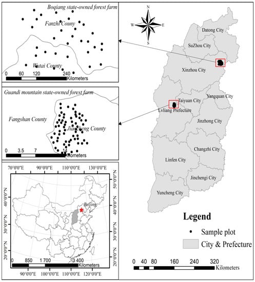
Figure 1.
Study area showing the sample plot location.
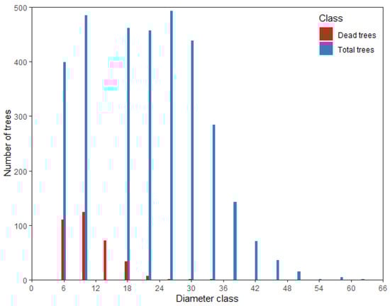
Figure 2.
Distribution pattern of forest mortality.
2.2. Selection of Predictor Variables
All the predictor variables that we evaluated for their potential contributions to tree mortality were grouped into the three sets based on the information related to tree- or stand- or climate-related mortality, (1) individual predictor tree variables (I): Diameter at breast height (D), tree height, ratio of diameter to average square diameter of stand (RD) and the sum of squares of tree diameters larger than the estimated diameter (DL); (2) stand predictor variables (S): Stand density (N), stand dominant height (DH), mean quadratic diameter (SMD) and RSI; (3) Climate predictor variables (C): Sixteen bioclimatic variables computed at the spatial resolution of 1 km × 1 km grids [50]. Climate data sets (1981–2012) were downloaded from the Climate AP based on the longitude, latitude, and elevation of each TSP. Data acquisition interval is one year. The definitions of all the climate variables are provided in Table 1. The mean values and the amplitude according to these predictor variables are given in Table 2.

Table 1.
Definition of climate variables.
Table 2.
Summary statistics of the variables at three levels. D: Diameter at breast height, H: Individual tree height, DL: Sum of squares of tree diameters greater than the estimated diameter, RD: Ratio of subject tree diameter to average square diameter of stand, N: Stand density, DH: Stand dominant height, SMD: Stand mean quadratic diameter, RSI: Relative spacing index, and the meanings of climate variables are shown in Table 1.
3. Model Development
3.1. Individual Tree Variables
The DL was calculated as a larger value than the sum of squares of the diameter of the target tree in a stand (Equation (1)). The RD was calculated as a ratio of diameter and stand mean square diameter (Equation (2)).
where and are the corresponding and of the tree on the sample plot nested within the block, () is the DBH of the () tree on the sample plot nested within the block, and is the number of observations in the sample plot nested within the block.
We dealt with the multiple collinearity problems between the predictor variables using the variance inflation factor (VIF). We retained the predictor variables with VIF < 5 in our final models, for example, D2, 1/D and other variables with VIF > 5 were excluded. In addition, DL and RD also significantly correlated with D, which could more effectively reflect the competition intensity than D, and therefore we excluded D from our final model.
3.2. Stand Variables
We chose widely used stand-level variables, such as dominant height and relative spacing index to fit the models. The index (Equation (3)) was calculated as suggested by Wyckoff and Clark [51].
where , , and are the , stand density (N, trees/ha) and dominant tree height (DH, m), respectively, of the sample plot nested within the block. The four dominant trees (four largest trees in a 400 m2 sample plot) were identified and measured. DH is arithmetic mean of four dominant heights [52].
3.3. Climate Variables
We evaluated the potential contributions of each climate variable (Table 1) to the description of the mortality variations. Only those variables, which were uncorrelated or less correlated or had VIF < 5 and contributed significantly to the descriptions of tree mortality were retained in the final model. With this selection approach, only two predictor variables—mean of difference in temperature (DT) and mean annual precipitation (MAP)—were found to significantly contribute to the mortality models, and were included as predictor variables in the extended mortality models.
As mentioned earlier, we developed the logistic mortality models through retaining only the significant predictor variables in the models. For an individual tree, it was convenient to fit the probability of survival with a binary response variable (living or dead, 1 or 0, respectively). A widely used function for precisely describing the binary data is the logistic model [13,53], which is expressed as,
where Pij is the probability of survival in the th sample plot nested in the th block, is the matrix vector of predictor variables used to fit the model, including individual, stand and climate variables, β0 is the intercept, and is the parameter vector.
By combining predictor variables at three different scales (individual tree, stand and climate), the advantages and disadvantages of the resulting models were compared. We built the models with combinations of the three scales of variables, such as I (only individual tree variables), S (only stand variables), C (only climate variables), I + S (individual tree and stand variables), S + C (stand and climate variables), I + S + C (individual tree, stand, and climate variables), and then selected the best among these combinations using the area under receiver operating curve (AUC), which the common statistical index used for model comparison. Then, we used the best one to establish the logistic two-level models through the Bayesian modeling.
3.4. Two-Level Models
Due to the hierarchical structure of data (trees in sample plots that are nested in a block). We established both the one- and two-level models: Block (level 1) and sample plot (level 2) level models. Let represent the level 1 unit (block) and represent the level 2 unit (plot); thus, a two-level random intercept logistic model is expressed as:
where is a two-level random effect assumed to have a normal distribution with mean 0 and variance . is a two-level random effect assumed to have a normal distribution with mean 0 and variance . and represent the random effects of the ith block and jth sample plot, respectively. are the fixed-effect parameters and are selected predictors.
To develop the models, fixed effects only, block random effects, and two-level random effects were included into the intercept, in addition to the three-level variables (individual, stand, and climate variables). Both the one- and two-level models were fitted to account for the autocorrelations of the observations in the block (level 1) with sample plot (level 2).
All the parameters of the Bayesian logistic models are estimated through the Markov chain Monte Carlo (MCMC) simulation using the R package MCMCglmm, which uses the combination of Gibbs sampling, slice sampling, and Metropolis–Hastings sampling [54]. We used “non-informative” priors for all the regression coefficients, i.e., a normal distribution with zero mean and a large variance (104). It is important to note that the posterior mean depends largely on the choice of the non-informative priors for the variance component, i.e., uniform (0, 1) and Inverse Gamma (0.001, 0.001) [53]). We set some parameters, such as the total number of iterations: 60,000 with a burn-in of 10,000 for tree mortality models. Additionally, thinning parameters were all set to 10 to reduce the autocorrelations and we chose the Inverse Gamma (0.001, 0.001) as the variance component.
The Akaike Information Criteria (AIC) was used to evaluate the fitting performance of models [55]. The smaller the AIC, the better the model fitting effect would be.
3.5. Model Evaluation
The Bayesian two-level models were compared with the Bayesian fixed-effect (non-hierarchical) models using the deviance information criterion (DIC) [55], which is calculated as:
where Q is some set of the model parameters and it is the effective number of parameters in the model, mean deviance () is calculated over all the iterations, and it is the posterior mean of the deviance, . is a point estimate of deviance given by . The advantage of DIC over other criteria in Bayesian model selection is that DIC can be easily calculated from samples generated by an MCMC simulation. Models with lower DIC values indicate a better fit to the data in which differences ≥5 are regarded as substantial evidence and differences ≥10 are regarded as very strong evidence in favor of the model with the lowest DIC [54].
The value of the area under the receiver operating curve (AUC) is a threshold-independent indicator to differentiate live and dead trees. The models with larger AUC values indicate a better fit to the data [56]. In general, an AUC value of 0.5 suggests no discrimination, 0.6–0.7 indicates poor discrimination, 0.7–0.8 suggests acceptable discrimination, and 0.8–0.9 stands for an excellent discrimination between live and dead trees [8]. The threshold is calculated by the ROCR package in R [57], which is used to determine that the predicted values of the developed models were 1 or 0. If the predicted values of tree mortality were greater than or equal to the corresponding threshold, the tree mortality would be equal to 1; otherwise, it would be equal to 0.
4. Results
4.1. Model Evaluation
The results showed that I, S, C, I + S, S + C, and I + S + C were the best model forms for simulating tree mortality through the Bayesian modeling with a combination of three levels of the predictor variables (Table 3). The models including individual variables (e.g., I, I + S, I + C, and I + S + C) showed the superior fit indices (higher AUC values) compared to other models (S, C, S + C), which had smaller AUC values. Thus, we considered only four models (I, I + S, I + C, I + S + C) with the individual predictor variables to develop both the one- and two-level models.
Table 3.
Model comparison and selection; AUC area under receiver operating characteristic.
4.2. Two-Level Mortality Model
As mentioned above, we only selected four alternatives (I, I + S, I + C, I + S + C) to include the random effects at one level and two levels into the tree mortality models. We chose the optimal threshold from the base models, the one-level model, and the two-level model. Then, we used the optimal threshold to calculate the AUC value for each model. For example, we chose a better threshold from the basic, one-level, and two-level models using individual level variables, and then we applied this threshold to the three models to calculate the AUC value.
The parameter estimates, associated standard deviations, DIC, and AUC for Bayesian fixed-effect (non-hierarchical), one-level, and two-level models are presented in Table 4. The fixed-effect parameter estimates in the multilevel models were larger than those in the fixed-effect models; therefore, ignoring the random effects underestimated most of the fixed-effect parameters.
Table 4.
Parameter estimates of tree survival models from fixed-effect (non-hierarchical: Base, one-level, and two-level random effects) models using the Bayesian method.
The DIC values of the Bayesian one-level and two-level models were much smaller than the base model, which indicates that both the one-level and two-level models are superior to the base model. Compared to the base model, the two-level model showed better-fit indexes (bigger AUC and smaller DIC). Compared to the different model by using different level predictor variables, the Bayesian two-level model showed superior fit indexes (smaller DIC and bigger AUC).
For the model constructed by the combination of predictor variables, for all forms of the components, AUC values of all models were greater than 0.8; thus, all the models were considered adequate in terms of their precisions.
In accordance with the base, one-level and two-level models of I (I + S, I + C, I + S + C), tree mortality significantly negatively correlated with RD and SMD, but positively correlated with DL. Two-level models showed the largest AUC and the smallest DIC.
4.3. Climate Effects on Tree Mortality
A summary of the parameter estimates obtained in the climate sensitive mortality models is provided in Table 4. Two climatic variables DT and MAP were significantly correlated with tree mortality. In the two-level models, DT had a negative effect on the mortality of Chinese fir. While the climate effects, including DT and MAP on the tree mortality were significant (Table 4), the effects were relatively small (Figure 3).
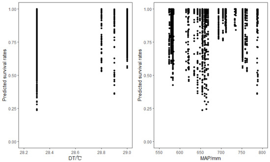
Figure 3.
Effects of climate variables on the predicted probabilities of survival in Prince Rupprecht larch (Larix gmelinii subsp. principis-rupprechtii).
5. Discussion
The Bayesian modeling method could adequately describe the phenomenon of variations at multiple clustering levels of data, such as the block or the sample plot level in the tree mortality analysis. Compared to the traditional modeling method, such as the ordinary least square regression and the maximum likelihood method, the Bayesian method has independent prior distributions to build the models [58]. Both the traditional and Bayesian methods have their own features in the modeling tree and stand characteristics. We did not intend to compare the Bayesian models against the traditional methods in details, as the latter modeling approach is not suitable for the hierarchical data structure. In particular, when the Bayesian prior is uninformative, the results of these two methods would be almost similar [59,60,61]. Thus, in this study, we chose the Bayesian modeling method, which is considered the best.
Several researchers have also reported that tree-level, stand-level, and climatic variables such as DBH, stand basal area, and mean annual temperature significantly contribute to tree mortality [10,23,62]. We also evaluated these variables; however, prediction precision of the resulting model did not significantly improve. The insignificant contributions of such variables to the mortality models may be due to the inherent collinearity among other variables that are included into the final models. Due to the uncertainties and complexity in the tree mortality process, we lacked an effective tool or method to determine a reasonable combination of tree-level, stand-level, and climatic variables and their interactions with the stand-specific conditions for predicting tree mortality.
A ratio of the diameter to the average square diameter of the stand (RD) had a negative correlation with tree mortality and the sum of squares of tree diameters greater than the estimated diameter (DL) had a positive correlation. With smaller RD and bigger DL, the probability of tree mortality would be smaller. This may be due to smaller RD and bigger DL in the same stand, indicating that the individual tree DBH is small. As the tree mortality rate generally decreases with increasing tree size, mortality rates can be higher for the juvenile trees, decrease with increasing tree size, and start to increase again with further increase of tree size [63]. Similarly, the effect of SMD (stand quadratic mean diameter) (size index) on tree mortality was negative (i.e., greater SMD, smaller stand mortality), indicating that tree mortality is more likely in the forests with many small trees compared to the forests with larger trees [64]. This finding is also consistent with the study [65], which shows that the mortality rate of young trees decreases with the increase of tree size and begins to increase when the mature age is reached. According to the local data survey [66], the mature age of Prince Rupprecht larch is 85 years. In this study, the data we collected were from natural secondary forests intervened in by human activities in the 1970s and all the trees almost did not reach mature age. In addition, Prince Rupprecht larch is a light-loving tree species. If young trees grown under the main forest layer obtain less light resource due tree crowding and intense competition, they would die easily.
Several existing studies show the climate warming-induced drought that might be the main driver of a widespread increase of tree mortality [13,67,68,69,70,71]. Our study confirms that DT and MAP, which were selected among the 16 bioclimatic predictor variables, have significant influences on tree mortality. A significant positive correlation with DT suggests that low mean temperature in the warmest month and high mean temperature in the coldest month increases tree mortality. Lower mortality is related to higher DT, and higher DT indicates a higher probability of the high temperature of the study area within the growing season, and hence the lower mortality rate [51,72]. This is also consistent with the findings from the Table 4 and Figure 3 that an increase in temperature increases the probability of survival (i.e., positive trend in Figure 3, and positive coefficients in Table 4).
Temperature affects tree growth and mortality by changing photosynthesis, respiration, cell division and elongation, chlorophyll synthesis, enzyme activity, water absorption, and transpiration [73]. Generally speaking, when the available water is not limited during the growing season, the increase of temperature difference physiologically reduces the probability of tree mortality. In this study, the temperature difference between day and night in the state-owned Guandi Mountain Larch forest and the state-owned Boqiang larch forest within the growing season of the Prince Rupprecht larch is small, and this means that the Prince Rupprecht larch grows in the environment of extreme high temperature for a long time, and the long-term extreme high temperature may increase the forest mortality. The main reasons for this may be that: (1) Increasing water shortage of trees and increasing drought pressure may directly or indirectly lead to tree mortality; (2) promotion of growth and reproduction of insects and pathogens attacking trees; (3) Prince Rupprecht larch trees situated close pores to prevent hydraulic failure (i.e., water column cavitation), which may lead to carbon starvation because high respiratory costs lead to depletion of carbon reserves [72]. The effect of drought caused by climate change on tree mortality is consistent with the recent drought in the withering event of the subtropical monsoon evergreen broad-leaved forest in southern China. In temperate forests in the western United States, a positive correlation was observed between the short-term change of forest loss and drought caused by climate change [19].
The significant positive correlations between the MAP and tree mortality (Table 4, Figure 3) may be due to the co-effects of temperature and precipitation on tree mortality [72]. In northern China, overall, the temperature of the wettest quarter is quite high, and there is the greatest amount of precipitation during the year [74]. However, Prince Rupprecht larch is a typically drought-resistant species in northern China [66]. Therefore, too much precipitation and too high temperature could inhibit physiological processes of the Prince Rupprecht larch and growth [75]. In addition, a large amount of precipitation also causes excessive nutrient loss by flooding [76]. These are the reasons that higher mortality is related to a greater MAP.
Compared to the mortality models built with the tree-level predictor variables, the improved method with the model built with the tree-level predictor variables could show better performance. With the smallest DIC and the biggest AUC, the Bayesian two-level model (I + S + C) was the best for predicting tree mortality of larch. This is similar to the results with the random intercept term included in the multilevel tree mortality models, which largely improved the fit index compared to the fixed-effect model [77]. Moreover, to effectively account for spatial correlations of our data, we preferred using the Bayesian modeling method. All three forms of the model (base, one-level, and two-level models), which were constructed using the Bayesian modeling approach, showed the excellent statistical indicators (AUC > 0.8). The influence of climate factors on the tree mortality are shown to be significant through modeling, and resulting mortality models can effectively assess the forest mortality under climate change.
6. Conclusions
We built the tree mortality models with the inclusion of tree-level, stand-level, and climatic predictor variables using the Bayesian modeling approach for Prince Rupprecht larch in northern China. The main conclusions are:
- (1)
- The best model included the predictor variables at three levels: Individual tree- and stand-, and environmental (climate)-levels in the Bayesian logistic models.
- (2)
- The Bayesian two-level model, which includes tree-level, stand-level, and climatic predictor variables, outperformed all the other forms of the models, describing larger variations of tree mortality and accounting for multiple sources of the unobserved heterogeneities.
- (3)
- Tree mortality significantly positively correlated with the sum of squares of tree diameters larger than the estimated diameter, and mean annual precipitation, but negatively correlated to the ratio of the diameter to the average square diameter of stand, the stand arithmetic mean diameter, and the mean of difference in temperature.
- (4)
- Presented mortality models will have significant implications for identifying different factors affecting tree mortality and precise prediction of the mortality.
- (5)
- With the mortality data collected from a wider distribution of the tree species of interest and advanced modeling techniques, the prediction performance of the tree mortality models may be improved, which we aim for in the future.
Author Contributions
L.X., X.C. and X.Z. collected data; L.X. and X.Z. analyzed data; L.X., X.C., R.P.S., X.Z. and J.L. wrote manuscript and contributed critically to improve the manuscript, and gave a final approval for publication. All authors have read and agreed to the published version of the manuscript.
Funding
This research was funded by the National Natural Science Foundations of China (No. 31971653).
Institutional Review Board Statement
Not applicable.
Informed Consent Statement
Not applicable.
Data Availability Statement
Data used in this study are available from the Chinese Forestry Science Data Center: http://www.cfsdc.org (accessed on 8 December 2020).
Acknowledgments
We are grateful to two anonymous reviewers, who provided the constructive comments and suggestions for improvement of the article.
Conflicts of Interest
The authors declare no conflict of interest.
References
- Zhang, X.; Lei, Y.; Cao, Q.V.; Chen, X.; Liu, X. Improving tree survival prediction with forecast combination and disaggregation. Can. J. For. Res. 2011, 41, 1928–1935. [Google Scholar] [CrossRef] [Green Version]
- Monserud, R.A.; Sterba, H. Modeling individual tree mortality for Austrian forest species. For. Ecol. Manag. 1999, 113, 109–123. [Google Scholar] [CrossRef]
- Eid, T.; Tuhus, E. Models for individual tree mortality in Norway. For. Ecol. Manag. 2001, 154, 69–84. [Google Scholar] [CrossRef]
- Yao, X.H.; Titus, S.J.; MacDonald, S.E. A generalized logistic model of individual tree mortality for aspen, white spruce, and lodgepole pine in Alberta mixedwood forests. Can. J. For. Res. 2001, 31, 283–291. [Google Scholar] [CrossRef]
- Das, A.J.; Stephenson, N.L. Improving estimates of tree mortality probability using potential growth rate. Can. J. For. Res. 2015, 45, 920–928. [Google Scholar] [CrossRef]
- Wyckoff, P.H.; Clark, J.S. Predicting tree mortality from diameter growth: A comparison of maximum likelihood and Bayesian approaches. Can. J. For. Res. 2000, 30, 156–167. [Google Scholar] [CrossRef]
- Adame, P.; Miren, D.R.; Caellas, I. Modeling individual-tree mortality in Pyrenean oak (Quercus pyrenaica Willd.) stands. Ann. For. Sci. 2010, 67, 1–10. [Google Scholar] [CrossRef]
- Chao, K.J.; Phillips, O.L.; Gloor, E.; Monteagudo, A.; Torres-Lezama, A.; Martinez, R.V. Growth and wood density predict tree mortality in Amazon forests. J. Ecol. 2008, 96, 281–292. [Google Scholar] [CrossRef]
- Crecente-Campo, F.; Marshall, P.; Rodríguez-Soalleiro, R. Modeling non-catastrophic individual-tree mortality for Pinus radiata plantations in northwestern Spain. For. Ecol. Manag. 2009, 257, 1542–1550. [Google Scholar] [CrossRef]
- Ruiz-Benito, P.; Lines, E.R.; Gómez-Aparicio, L.; Zavala, M.A.; Coomes, D.A. Patterns and drivers of tree mortality in Iberian forests: Climatic effects are modified by competition. PLoS ONE 2013, 8, e56843. [Google Scholar] [CrossRef] [Green Version]
- Adams, H.D.; Guardiola-Claramonte, M.; Barron-Gafford, G.A.; Villegas, J. Temperature sensitivity of drought-induced tree mortality portends increased regional die-off under global-change-type drought. Proc. Natl. Acad. Sci. USA 2009, 106, 7063–7066. [Google Scholar] [CrossRef] [Green Version]
- Ma, Z.; Lei, X.; Zhu, Q.; Cheng, H.; Peng, C. A drought-induced pervasive increase in tree mortality across Canada’s boreal forests. Nat. Clim. Chang. 2011, 1, 467–471. [Google Scholar]
- Brando, P.M.; Balch, J.K.; Nepstad, D.C.; Morton, D.C.; Putz, F.E.; Coe, M.T.; Silverio, D.; Macedo, M.N.; Davidson, E.A.; Nobrega, C.C. Abrupt increases in Amazonian tree mortality due to drought–fire interactions. Proc. Natl. Acad. Sci. USA 2014, 111, 6347. [Google Scholar] [CrossRef] [PubMed] [Green Version]
- Zhang, X.Q.; Cao, Q.V.; Duan, A.G.; Zhang, A.G. Modeling tree mortality in relation to climate, initial planting density and competition in Chinese fir plantations using a Bayesian logistic multilevel method. Can. J. For. Res. 2017, 49, 1278–1285. [Google Scholar] [CrossRef]
- Qiu, S.; Xu, M.; Xu, R.Q.; Li, Y.P.; Zheng, Y.; Daniel, C.; Cui, X.W.; Cui, L.X.; Liu, C.H.; Zhang, L.W.; et al. Climatic information improves statistical individual-tree mortality models for three key species of Sichuan Province, China. Ann. For. Sci. 2015, 72, 443–455. [Google Scholar] [CrossRef] [Green Version]
- Zhang, X.Q.; Lei, Y.C.; Liu, X.Z. Modeling stand mortality using Poisson mixture models with mixed-effects. Ifor.-Biogeosci. For. 2015, 8, 333–338. [Google Scholar] [CrossRef]
- Lutz, J.A.; Halpern, C.B. Tree mortality during early forest development: A long-term study of rates, causes, and consequences. Ecol. Monogr. 2006, 76, 257–275. [Google Scholar] [CrossRef]
- Larson, A.J.; Franklin, J.F. The tree mortality regime in temperate old-growth coniferous forests: The role of physical damage. Can. J. For. Res. 2010, 40, 2091–2103. [Google Scholar] [CrossRef] [Green Version]
- Van Mantgem, P.J.; Stephenson, N.L.; Byrne, J.C.; Daniels, L.D.; Franklin, J.F.; Fule, P.Z.; Harmon, M.E.; Larson, A.J.; Smith, J.M.; Taylor, A.H.; et al. Widespread increase of tree mortality rates in the western United States. Science 2009, 323, 521–524. [Google Scholar] [CrossRef] [Green Version]
- Hamilton, D.A. Event Probabilities Estimated by Regression; Intermountain Forest & Range Experiment Station, Forest Service, US Department of Agriculture: Fort Collins, CO, USA, 1974. [Google Scholar]
- Weingartner, M.M. Estimating tree mortality of Norway spruce stands with neural networks. Adv. Environ. Res. 2001, 5, 405–414. [Google Scholar]
- Rose, C.E., Jr.; Hall, D.B.; Shiver, B.D.; Clutter, M.L.; Borders, B. A multilevel approach to individual tree survival prediction. For. Sci. 2006, 52, 31–43. [Google Scholar]
- Yang, Y.; Titus, S.J.; Huang, S. Modeling individual tree mortality for white spruce in Alberta. Ecol. Model. 2003, 163, 209–222. [Google Scholar] [CrossRef]
- Boeck, A.; Dieler, J.; Biber, P.; Pretzsch, H.; Ankerst, D.P. Predicting tree mortality for European beech in southern Germany using spatially explicit competition indices. For. Sci. 2014, 60, 613–622. [Google Scholar] [CrossRef]
- Coble, D.W.; Cao, Q.V.; Jordan, L. An Annual Tree Survival and Diameter Growth Model for Loblolly and Slash Pine Plantations in East Texas. South. J. Appl. For. 2012, 36, 79–84. [Google Scholar] [CrossRef]
- Moser, J.W. Dynamics of an Uneven-Aged Forest Stand. For. Sci. 1972, 18, 184–191. [Google Scholar]
- Hamilton, D.A., Jr. Extending the range of applicability of an individual tree mortality model. Can. J. For. Res. 1990, 20, 1212–1218. [Google Scholar] [CrossRef]
- Adams, H.D.; Williams, A.P.; Xu, C.; Rauscher, S.A.; Jiang, X.; McDowell, N.G. Empirical and process-based approaches to climate-induced forest mortality models. Front. Plant Sci. 2013, 4, 438. [Google Scholar] [CrossRef] [Green Version]
- Somers, G.L.; Oderwald, R.G.; Harms, W.R.; Langdon, O.G. Predicting Mortality with a Weibull Distribution. For. Sci. 1980, 26, 291–300. [Google Scholar]
- Holzwarth, F.; Kahl, A.; Bauhus, J.; Wirth, C. Many ways to die—Partitioning tree mortality dynamics in a near-natural mixed deciduous forest. J. Ecol. 2013, 101, 220–230. [Google Scholar] [CrossRef]
- Buford, M.A.; Hafley, W.L. Probability distributions as models for mortality. For. Sci. 1985, 31, 331–341. [Google Scholar]
- Kobe, R.K.; Coates, K.D. Models of sapling mortality as a function of growth to characterize interspecific variation in shade tolerance of eight tree species of northwestern British Columbia. Can. J. For. Res. 1997, 27, 227–236. [Google Scholar] [CrossRef]
- Travis, W.; Shaw, D.C.; Ganio, L.M.; Fitzgerald, S. A review of logistic regression models used to predict post-fire tree mortality of western North American conifers. Int. J. Wildland Fire 2012, 21, 1–35. [Google Scholar]
- Zeng, Z.; Yin, G.; Zhang, Y.; Sun, Y.; Wang, T.; Piao, S. MODIS based estimation of forest aboveground biomass in China. PLoS ONE 2015, 10, e0130143. [Google Scholar] [CrossRef] [Green Version]
- Fu, L.; Zhang, H.; Sharma, R.P.; Pang, L.; Wang, G. A generalized nonlinear mixed-effects height to crown base model for Mongolian oak in northeast China. For. Ecol. Manag. 2017, 384, 34–43. [Google Scholar] [CrossRef]
- Fu, L.; Lei, Y.; Affleck, D.L.; Nelson, A.S.; Shen, C.; Wag, M.; Zheng, J.; Ye, Q.; Yang, G. Additivity of nonlinear tree crown width models: Aggregated and disaggregated model structures using nonlinear simultaneous equations. For. Ecol. Manag. 2018, 427, 372–382. [Google Scholar]
- West, P.W.; Ratkowsky, D.A.; Davis, A.W. Problems of hypothesis testing of regressions with multiple measurements from individual sampling units. For. Ecol. Manag. 1984, 7, 207–224. [Google Scholar] [CrossRef]
- Chen, D.; Huang, X.; Sun, X.; Ma, W.; Zhang, S. A Comparison of Hierarchical and Non-Hierarchical Bayesian Approaches for Fitting Allometric Larch (Larix. spp.) Biomass Equations. Forests 2016, 7, 18. [Google Scholar] [CrossRef] [Green Version]
- Mauricio, Z.C.; Carlos, A.S.; Lauren, A. Probability distribution of allometric coefficients and Bayesian estimation of aboveground tree biomass. For. Ecol. Manag. 2012, 277, 173–179. [Google Scholar]
- Zhang, X.; Zhang, J.; Duan, A. A Hierarchical Bayesian Model to Predict Self-Thinning Line for Chinese Fir in Southern China. PLoS ONE 2015, 10, e0139788. [Google Scholar]
- Zhang, X.; Duan, A.; Zhang, J. Tree Biomass Estimation of Chinese fir (Cunninghamia lanceolata) Based on Bayesian Method. PLoS ONE 2013, 8, e79868. [Google Scholar] [CrossRef] [Green Version]
- Anholt, B.R.; Werner, E.; Skelly, D.K. Effect of Food and Predators on the Activity of Four Larval Ranid Frogs. Ecology 2000, 81, 3509–3521. [Google Scholar] [CrossRef]
- Leng, W.F.; He, H.S.; Liu, H.J. Response of larch species to climate changes. J. Plant Ecol. 2008, 1, 203–205. [Google Scholar] [CrossRef] [Green Version]
- Tao, B.; Cao, M.K.; Gui, R.; Liu, J.Y.; Wang, S.Q. Global Carbon Project (GCP) Beijing Office: A new bridge for understanding regional carbon cycles. J. Geogr. Inf. Syst. 2006, 016, 375–377. [Google Scholar]
- Chen, H.; Xu, Z.B. Preliminary study on the tree death of Korean pine deciduous mixed forest of Changbai Mountain. Chin. J. Appl. Ecol. 1991, 2, 89–91. [Google Scholar]
- Ban, Y.; Xu, H.C.; Li, Z.D. Mortality patterns of Larix gmelini and effect of fallen dead wood on regeneration of old Larixgmeliforest. Chin. J. Appl. Ecol. 1997, 8, 449. [Google Scholar]
- Chambers, J.Q.; Negron-Juarez, R.I.; Marra, D.M.; Di Vittorio, A.; Tews, J.; Roberts, D.; Ribeiro, G.H.; Trumbore, S.E.; Higuchi, N. The steady-state mosaic of disturbance and succession across an old-growth Central Amazon forest landscape. Proc. Natl. Acad. Sci. USA 2013, 110, 3949–3954. [Google Scholar] [CrossRef] [PubMed] [Green Version]
- Erb, K.H.; Fetzel, T.; Plutzar, C.; Kastner, T.; Lauk, C.; Mayer, C.; Niedertscheider, M.; KöRner, C.; Haberl, H. Biomass turnover time in terrestrial ecosystems halved by land use. Nat. Geosci. 2016, 9, 674–678. [Google Scholar] [CrossRef]
- Lewis, S.L.; Brando, P.M.; Phillips, O.L.; van der Heijden, G.M.; Nepstad, D. The 2010 Amazon drought. Science 2011, 331, 554. [Google Scholar] [CrossRef]
- Wang, T.; Hamann, A.; Spittlehouse, D.L.; Murdock, T.Q. Climate WNA—High-resolution spatial climate data for western north America. J. Appl. Meteorol. Climatol. 2012, 51, 16–29. [Google Scholar] [CrossRef] [Green Version]
- Wyckoff, P.H.; Clark, J.S. The relationship between growth and mortality for seven co-occurring tree species in the southern Appalachian Mountains. J. Ecol. 2002, 90, 604–615. [Google Scholar] [CrossRef] [Green Version]
- Raulier, F.; Lambert, M.; Pothier, D.; Ung, C. Impact of dominant tree dynamics on site index curves. For. Ecol. Manag. 2003, 184, 65–78. [Google Scholar] [CrossRef]
- Akinwande, M.O.; Dikko, H.G.; Samson, A. Variance Inflation Factor: As a Condition for the Inclusion of Suppressor Variable(s) in Regression Analysis. Open J. Stat. 2015, 5, 754–767. [Google Scholar] [CrossRef] [Green Version]
- Li, B.; Lingsma, H.F.; Steyerberg, E.W.; Lesaffre, E. Logistic random effects regression models: A comparison of statistical packages for binary and ordinal outcomes. BMC Med. Res. Methodol. 2011, 11, 77. [Google Scholar] [CrossRef] [Green Version]
- Spiegelhalter, D.J.; Best, N.G.; Carlin, B.P.; van der Linde, A. Bayesian measures of model complexity and fit. J. R. Stat. Soc. Ser. B 2002, 64, 583–639. [Google Scholar] [CrossRef] [Green Version]
- Hurst, J.M.; Allen, R.B.; Coomes, D.A.; Duncan, R.P. Size-specific tree mortality varies with neighbourhood crowding and disturbance in a Montane Nothofagus forest. PLoS ONE 2011, 6, e26670. [Google Scholar] [CrossRef] [PubMed] [Green Version]
- R Core Team. R: A Language and Environment for Statistical Computing; R Foundation for Statistical Computing: Vienna, Austria, 2013; Available online: http://www.R-project.org/ (accessed on 31 March 2021).
- Zweig, M.H.; Campbell, G. Receiver-operating characteristic (ROC) plots: A fundamental evaluation tool in clinical medicine. Clin. Chem. 1993, 39, 561–577. [Google Scholar] [CrossRef]
- Pinheiro, J.C.; Bates, D.M. Mixed-Effects Models in S and S-PLUS; Springer Science & Business Media: Berlin, Germany, 2006. [Google Scholar]
- Mueller, R.C.; Scudder, C.M.; Porter, M.E.; Talbot Trotter, R., III; Gehring, C.A.; Whitham, T.G. Differential tree mortality in response to severe drought: Evidence for long-term vegetation shifts. J. Ecol. 2005, 93, 1085–1093. [Google Scholar] [CrossRef]
- Mccarthy, M.A. Bayesian Methods for Ecology; Cambridge University Press: Cambridge, UK, 2007. [Google Scholar]
- Wunder, J.; Reineking, B.; Matter, J.F.; Bigler, C.; Bugmann, H. Predicting tree death for Fagus sylvatica and Abies alba using permanent plot data. J. Veg. Sci. 2010, 18, 525–534. [Google Scholar] [CrossRef]
- Ma, Z.; Peng, C.; Li, W.; Zhu, Q.; Wang, W.; Song, X.; Liu, J. Modeling individual tree mortality rates using marginal and random effects regression models. Nat. Resour. Modeling 2013, 26, 131–153. [Google Scholar] [CrossRef]
- Lorimer, C.G.; Frelich, L.E. A Simulation of Equilibrium Diameter Distributions of Sugar Maple (Acer saccharum). Bull. Torrey Bot. Club 1984, 111, 193–199. [Google Scholar] [CrossRef] [Green Version]
- Zhou, X.; Chen, Q.; Sharma, R.P.; Wang, Y.; He, P.; Guo, J.; Lei, Y.; Fu, L. A climate sensitive mixed-effects diameter class mortality model for Prince Rupprecht larch (Larix gmelinii var. principis-rupprechtii) in northern China. For. Ecol. Manag. 2021, 491, 119091. [Google Scholar] [CrossRef]
- Zhang, Z.X. Dendrology (The North), 2nd ed.; China Forestry Publishing House: Beijing, China, 2010. (In Chinese) [Google Scholar]
- Buchman, R.G.; Pederson, S.P.; Walters, N.R. A tree survival model with application to species of the Great Lakes region. Can. J. For. Res. 1983, 13, 601–608. [Google Scholar] [CrossRef]
- Martínezvilalta, J.; Pinol, J. Drought-induced mortality and hydraulic architecture in pine populations of the NE Iberian Peninsula. For. Ecol. Manag. 2002, 161, 247–256. [Google Scholar] [CrossRef]
- Juknys, R.; Vencloviene, J.; Jurkonist, N.; Bartkevicius, E.; Sepetiene, J. Relation between Individual Tree Mortality and Tree Characteristics in a Polluted and Non-Polluted environment. Environ. Monit. Assess. 2006, 121, 519–542. [Google Scholar] [CrossRef] [PubMed]
- McDowell, N.; Pockman, W.T.; Allen, C.D.; Breshears, D.D.; Cobb, N.; Kolb, T.; Yepez, E.A. Mechanisms of plant survival and mortality during drought: Why do some plants survive while others succumb to drought? New Phytol. 2008, 178, 719–739. [Google Scholar] [CrossRef]
- Allen, C.D.; Macalady, A.K.; Chenchouni, H.; Bachelet, D.; McDowell, N.; Vennetier, M.; Cobb, N. A global overview of drought and heat-induced tree mortality reveals emerging climate change risks for forests. For. Ecol. Manag. 2010, 259, 660–684. [Google Scholar] [CrossRef] [Green Version]
- Fu, L.; Sun, W.; Wang, G. A climate-sensitive aboveground biomass model for three larch species in northeastern and northern China. Trees 2017, 31, 557–573. [Google Scholar] [CrossRef]
- Ricker, M.; Gutiérrez-García, G.; Daly, D.C. Modeling long-term tree growth curves in response to warming climate: Test cases from a subtropical mountain forest and a tropical rainforest in Mexico. Can. J. For. Res. 2007, 37, 977–989. [Google Scholar] [CrossRef]
- Li, Y.; Sun, W.; Zhu, H.; Zhao, X.; Bai, Y.; Zhang, Y. Multi-time scale analysis on the variations of temperature and precipitation of main urban in Northeast of China. Sci. Tech. Eng. 2015, 15, 23–31. [Google Scholar]
- Wang, X.; Zhao, C.; Jia, Q. Impacts of climate change on forest ecosystems in Northeast China. Adv. Clim. Chang. Res. 2013, 4, 230–241. [Google Scholar]
- Chen, Y.; Song, X.; Zhang, Z.; Shi, P.; Tao, F. Simulating the impact of flooding events on non-point source pollution and the effects of fifilter strips in an intensive agricultural watershed in China. Limnology 2015, 16, 91–101. [Google Scholar] [CrossRef]
- Kurz, W.A.; Dymond, C.C.; Stinson, G.; Rampley, G.J.; Safranyik, L. Mountain pine beetle and forest carbon feedback to climate change. Nature 2008, 452, 987–990. [Google Scholar] [CrossRef] [PubMed]
Publisher’s Note: MDPI stays neutral with regard to jurisdictional claims in published maps and institutional affiliations. |
© 2022 by the authors. Licensee MDPI, Basel, Switzerland. This article is an open access article distributed under the terms and conditions of the Creative Commons Attribution (CC BY) license (https://creativecommons.org/licenses/by/4.0/).