Article

Dynamics Modeling and Hydrodynamic Coefficients Identification of the Wave Glider

1
Physical Oceanography Laboratory, Ocean University of China, Qingdao 266100, China
2
Tianjin Key Laboratory of Advanced Mechatronic Equipment Technology, School of Mechanical Engineering, Tiangong University, Tianjin 300387, China
3
Institute for Advanced Ocean Study, Ocean University of China, Qingdao 266100, China
*
Authors to whom correspondence should be addressed.
J. Mar. Sci. Eng. 2022, 10(4), 520; https://doi.org/10.3390/jmse10040520
Submission received: 28 January 2022 / Revised: 28 March 2022 / Accepted: 3 April 2022 / Published: 8 April 2022
(This article belongs to the Section Ocean Engineering)

Abstract

:
The wave glider is an ocean-wave-propelled autonomous marine vehicle with unique dual-body architecture, which can converse the energy obtained from the ocean wave into the forward thrust. In this paper, the dynamic models of the submerged glider based on dynamic characteristics of tandem hydrofoils and the surface float were separately established. The pitching angles of the hydrofoils and the submerged glider and the angle of attack between hydrofoils and relative current were considered for dynamic models and hydrodynamic coefficients. The translational hydrodynamic coefficient term for high-angle-of-attack passive motion of the submerged glider was calculated from static test simulations by using Computational Fluid Dynamics (CFD). Moreover, the rotational damping coefficients and added mass coefficients varying with the pitching angle of hydrofoils were analyzed by the simulation of the vertical planar motion mechanism (VPMM) tests. Furthermore, the numerical simulation of longitudinal motion with the computed hydrodynamic coefficients was performed, and the simulation results were compared with the sea trial data. The analysis was performed, and conclusions were drawn, which would provide a theoretical reference for the design of the wave glider.

1. Introduction

In the 21st century, marine resources play an important role in supporting world economic prosperity. Numerous unmanned marine platforms are developing at an incredible pace. The wave glider invented by Robert Hine [1] is an ocean-wave-propelled autonomous marine vehicle which uses wave energy for propulsion and solar energy for onboard sensors and control and communication systems, etc. In comparison with other marine platforms, the wave glider has longer endurance and lower cost and has been widely applied to various marine scientific research in recent years.
The wave glider is composed of a submerged glider, a surface float and an umbilical cable, and its energy conversion system using wave energy is based on a dual-body design. When the surface float makes a heave motion in surface waves, the submerged glider also makes a heave motion by the umbilical cable. When the submerged glider rises, the hydrofoils rotate counterclockwise, and when the submerged glider falls, the hydrofoils rotate clockwise, as shown in Figure 1. The hydrodynamic forces generated by the relative movement between hydrofoils and seawater can be divided into vertical force and forward force. The forward hydrodynamic force will drive the wave glider forward.
Some researchers analyzed the hydrodynamic performance of tandem hydrofoils as the propulsor of the wave glider considering some factors such as oscillation amplitude and torsional spring stiffness [2,3,4,5]. Moreover, some researchers used numerical simulation based on the mathematical model for performance evaluation of the wave glider. Kraus and Bingham proposed a two-dimensional model of the wave glider in the along-track and heave directions, which was simplified as a coupled rigid body [6]. Kraus constructed a 6-DOF (Degree of Freedom) nonlinear dynamic model and identified several key hydrodynamic coefficients by using analytical and experimental methods [7]. Qi et al. established a 3-DOF dynamic model in the longitudinal plane by the Kane method [8]. Li et al., respectively, established the models of the surface float, the submerged glider and the connection umbilical based on multi-body dynamic theory and completed the motion simulation by using ADAMS and MATLAB [9]. Rampersadh described a multi-body system of the wave glider using Denavit–Hartenberg parametrization and established the dynamic model for bodies by using the Lagrangian approach [10]. Wang et al. presented a 4-DOF model of the wave glider, which included the second-order wave drift force on the horizontal plane and the first-order wave force in the vertical direction [11]. Chen et al. described a nonlinear kinetic model in three reference coordinate frames with 6-DOF, analyzed the static stress and optimized the hydrodynamics of the hydrofoil structure [12]. L. Wang et al. established a dynamic model of the wave glider based on the analysis of the state transfer problem of the umbilical [13].
The above-mentioned research works assume that the hydrodynamic performances are almost not influenced by the pitching angles of the hydrofoils and the submerged glider, and it is convenient to analyze the propulsive performance of the submerged glider. However, for the hinge joint between the umbilical and the submerged glider, the moment of the submerged glider is unbalanced in the actual sailing. Under the action of restoring the moment and hydrodynamic moment of the submerged glider, it causes a periodical change of the pitching angle of the submerged glider in a certain range. Due to the hydrofoils pivoted on the submerged glider, the pitching angle of the submerged glider is also an important factor for the hydrodynamic propulsion performance of the wave glider. The aforementioned research works also assume that added mass coefficients are constant and several coupled added mass coefficients of the submerged glider are ignored. However, due to the dynamic change of the hydrofoil during the motion of the wave glider, added mass coefficients are dependent on the body’s geometry and will change with the pitching angle of the hydrofoils.
The key step in numerical simulation is to determine the hydrodynamic coefficients applied in the mathematical model. With the rapid development of computing technology, it is feasible to analyze fluid–structure interaction problems based on CFD. Slone proposed a three-dimensional finite volume, unstructured mesh (FV-UM) method for dynamic fluid–structure interaction [14]. Westphalen, respectively, simulated the wave-structure interaction and wave loading by using the Finite Volume (FV) method, Control-Volume Finite Element (CV-FE) method, Smoothed Particle Hydrodynamics (SPH) and Cartesian Cut Cell method [15]. The Eulerian mesh method is limited by the grid size, but SPH is not limited, and it is better able to capture the jet. Ren proposed a two-dimensional SPH-DEM model to simulate the wave-structure interaction on a slope and predict the hydraulic stability of the 2D structure [16]. Xiang simulated the fluid impact forces on a bridge superstructure in the horizontal and vertical directions using the Finite Element-based Arbitrary Lagrangian–Eulerian Method [17]. Hasanpour presented a coupled SPH–FEM modeling approach that simulated the fluid with particles, and the flume, the debris and the structure with mesh-based finite elements [18]. Past studies have identified the importance and complexity of the dynamic fluid–structure interaction for different types of marine structures and this effect will be thoroughly investigated for wave gliders in our future research.
For hydrodynamic coefficients, CFD simulation is also more accurate compared to analytical and semi-empirical methods for complex shapes. Zhang et al. proposed a new method by using dynamic meshes in FLUENT to simulate hydrodynamic tests to obtain corresponding hydrodynamic coefficients of autonomous underwater vehicle (AUV) [19]. Malik and Guang obtained hydrodynamic coefficients for 6:1 prolate spheroid by simulating the planar motion mechanism (PMM) tests [20]. They maintained the domain mesh qualities during the movement of the rigid body by using three different mesh updating schemes and zoning of the computational field. Towing tests, PMM tests and rotating arm tests were simulated to obtain the hydrodynamic coefficients of AUV [21]. Singh et al. used CFD to estimate the hydrodynamic coefficients of an underwater glider, which was verified by comparing the experimental data of the gliding trajectory with the simulation results [22].
In this paper, the dynamic models of the surface float, the submerged glider with the hydrofoils and the umbilical were separately established in Section 2, which considered the influences of the dynamic variation of the pitching angles of the hydrofoils and the submerged glider. In Section 3, the hydrodynamic coefficients varying with the pitching angle of the hydrofoils were analyzed from static test simulations and dynamic PMM test simulations in FLUENT by using the Finite Volume Method (FVM). In Section 4, sea trial with the “Black Pearl” wave glider was conducted, and the numerical simulations under different sea conditions were carried out to predict the longitudinal velocity of the wave glider and the pitching angle of the submerged glider. The simulation results were reasonable by comparing with the sea trial data. Eventually, some conclusions were summarized in Section 5.

2. Dynamic Models of the “Black Pearl” Wave Glider

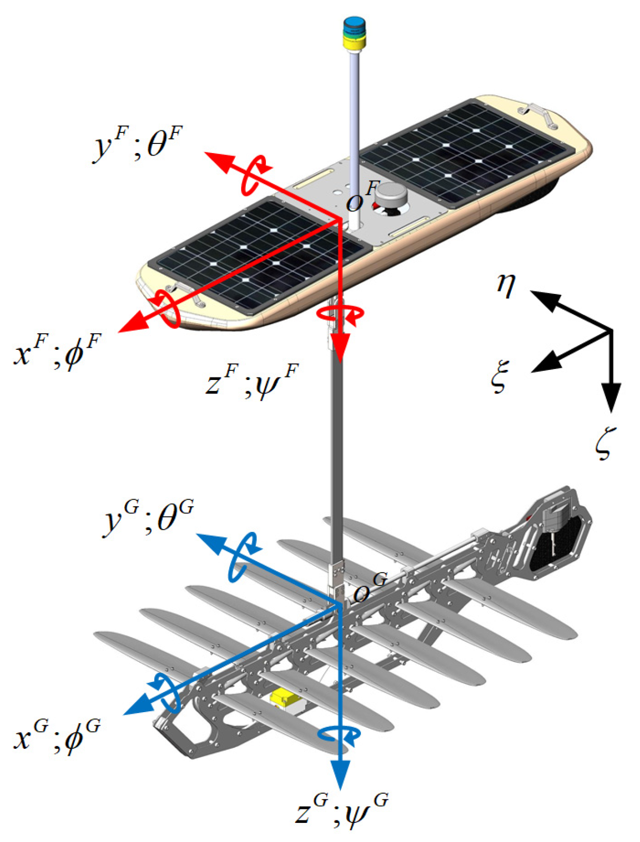
2.1. The Reference Frames

To facilitate modeling, three coordinate systems based on the right-handed rule were defined [10], as shown in Figure 2.
(1)
Float frame (with the right-superscript F): the hinge point between the surface float and the umbilical is as the origin of the coordinate frame. x F , y F and z F are positive toward the bow, the starboard and the bottom of the surface float, respectively;
(2)
Glider frame (with the right-superscript G): the hinge point between the submerged glider and the umbilical is as the origin of the glider frame. x G , y G and z G positive toward the bow, the starboard and the bottom of the submerged glider, respectively;
(3)
Inertial reference frame ( ξ η ζ ): ξ , η and ζ point toward north, east and downwards, respectively.

2.2. Dynamic Model of the Surface Float

Xiang revealed a great dependence of the wave loads on the ratio of wavelength to structure width [23]. Rudman used the Smoothed Particle Hydrodynamics (SPH) technique to simulate the influence on a semi-submersible platform at a range of different angles [24]. The interaction between the surface float and wave was simplified and the wave incident angle was assumed to be zero in this study. Moreover, due to the difficulty of predicting numerically irregular waves in the experimental sea area, the surface waves were assumed as regular waves. However, future studies will consider more realistic conditions, such as irregular waves and breaking waves or bores. The latter type of waves is challenging because they can be dominated by significant turbulence effects, air-entrapment and high-aleatory uncertainty [25,26,27] and can introduce totally different hydrodynamic loads compared to unbroken waves [28,29].
The heave motion of the surface float is assumed as a sinusoidal motion with surface waves. The longitudinal model of the surface float is formulated as follows [30]:
( M R B F + M A F ) ν ˙ F + C R B F ( ν F ) ν F + C A F ( ν r F ) ν r F + D F ( ν r F ) ν r F = τ w a v e F + τ 1 _ u m b
where M R B F and M A F are the inertia matrix and the added mass matrix of the surface float in the rigid-body system, respectively. ν F is the velocity vector of the surface float and ν r F is the velocity vector of the surface float relative to ocean current. C R B F ( ν F ) is the rigid-body Coriolis and Centripetal matrix of the surface float and C A F ( ν F ) is the hydrodynamic Coriolis and Centripetal matrix of the surface float. D F ( ν F ) is the damping matrix of the surface float, τ 1 _ u m b is the vector of umbilical force and τ w a v e F is the vector of wave force on the surface float.
The wave force is simply considered as an excitation force, which can be described as:
τ w a v e F = f w A w cos ( ω w t + φ w )
where f w is the wave force per unit wave amplitude, A w is the amplitude of wave high, ω w is the wave excitation frequency, and φ w is the phase.

2.3. Dynamic Model of the Submerged Glider

The longitudinal 3-DOF (surge, heave and pitch) coupled model of the submerged glider can be expressed as:
( M R B G + M A G ) ν ˙ G + C R B G ( ν G ) ν G + C A G ( ν r G ) ν r G + D G ( ν r G ) ν r G + g ( η ) = τ 2 _ u m b + τ h f
where M R B G and M A G are the inertia matrix and the added mass matrix of the submerged glider in the rigid-body system, respectively. ν G is the velocity vector of the submerged glider and ν r G is the velocity vector of the submerged glider relative to the ocean current. C R B G ( ν G ) is the rigid-body Coriolis and Centripetal matrix of the submerged glider and C A G ( ν G ) is the hydrodynamic Coriolis and Centripetal matrix of the submerged glider. D G ( ν G ) is the hydrodynamic damping matrix of the submerged glider and g ( η ) is the vector of restoring forces and moment of the submerged glider. τ 2 _ u m b is the vector of umbilical force on the submerged glider and τhf is the vector of hydrodynamic forces and moment of the hydrofoils.
The submerged glider is symmetric about the xz-plane and longitudinal motion is only considered; thus M R B G , M A G , C R B G ( ν G ) and C A G ( ν G ) are, respectively, simplified as:
M R B G = [ m G 0 m G z g G 0 m G m G x g G m G z g G m G x g G I y G ]
M A G = [ X u ˙ G X w ˙ G X q ˙ G Z u ˙ G Z w ˙ G Z q ˙ G M u ˙ G M w ˙ G M q ˙ G ]
C R B G ( ν G ) = [ 0 0 m ( x g G q G w G ) 0 0 m ( z g G q G + u G ) m G ( x g G q G w G ) m ( z g G q G + u G ) 0 ]
C A G = [ 0 0 a 3 G 0 0 a 1 G a 3 G a 1 G 0 ]
and the coefficients of the hydrodynamic Coriolis and Centripetal matrix of the submerged glider ( a 1 G and a 3 G ) are, respectively, written as:
a 1 G = X u ˙ G u r G + X w ˙ G w r G + X q ˙ G q G
a 3 G = Z u ˙ G u r G + Z w ˙ G w r G + Z q ˙ G q G
Hydrodynamic damping matrix D G ( ν r G ) includes the linear part DG and the nonlinear part D n G ( ν r G ) . D n G ( ν r G ) only includes additional nonlinear damping terms on the diagonal in surge and heave because other coupling terms are small, which are ignored in this model. Thus, D G and D n G ( ν r G ) are, respectively, expressed as:
D G = [ X u G X w G X q G Z u G Z w G Z q G M u G M w G M q G ]
D n G ( ν r G ) = diag { X | u | u G | u r G | , Z | w | w G | w r G | , 0 }
The vector of restoring force and moment g ( η ) is derived as:
g ( η ) = [ ( W G B G ) sin θ G ( W G B G ) cos θ G ( z g G W G z b G B G ) sin θ G + ( x g G W G x b G B G ) cos θ G ]
where W G and B G are the weight and the buoyancy force of the submerged glider, respectively.
The lift force ( F L ) and drag force ( F D ) of six pairs of tandem hydrofoils are obtained by the simulation. The vectors of drag and lift forces change with the vector of flow velocity, which is shown in Figure 3. During the falling phase of the glider, the drag force and the lift force of the hydrofoils in simulations can be resolved to the horizontal and vertical forces in the glider frame, which can be expressed as:
F h f x = F L sin θ ν G F D cos θ ν G F h f z = F L cos θ ν G F D sin θ ν G
During the rising phase of the glider, the drag force and the lift force of the hydrofoils in simulations can be resolved to the horizontal and vertical forces in the glider frame, which can be expressed as:
F h f x = F L sin θ ν G F D cos θ ν G F h f z = F L cos θ ν G + F D sin θ ν G
The vector of hydrodynamic forces and moment of the hydrofoils can be written as:
τ h f = [ F h f x F h f z M h f G ] T
where M h f G is the hydrodynamic moment of the hydrofoils acting on the submerged glider.
Figure 4 shows the force diagram of the hydrofoil, which mainly includes the hydrostatics, hydrodynamic force and spring tension. The pitching acceleration of the hydrofoils can be expressed as:
( I h f + M q ˙ h f ) θ ¨ h f G = M h f + M g M s
where I h f , M q ˙ h f , M q ˙ h f , M h f and M g are the inertia moment, the pitch added mass coefficient, the hydrodynamic moment and the gravitational/buoyancy moment of a pair of tandem hydrofoils, respectively. M s is the spring-induced moment.
M h f , M g and M s are respectively expressed as:
M h f = ( F h f x sin θ h f G + F h f z cos θ h f G ) L f
M g = ( m h f g B h f ) L f cos ( θ h f G + θ G n )
M s = k s Δ L s p L s sin ( θ h f G + θ s G )
where θ h f G is the pitching angle of the hydrofoils in the glider frame, θ G n the pitching angle of the submerged glider in the inertial reference frame, θ s G is the angle between the positive x-axis of the submerged glider and the spring, L f is the distance from the center of mass of a single pair of tandem hydrofoils to their pivot, L s is the distance from the pin attached to the spring to the pivot, k s is the spring stiffness coefficient, and Δ L s p is the elongation of the spring. θ s G can be expressed as:
θ s G = arctan ( h p + L s sin ( θ h f G ) L p L s cos ( θ h f G ) )
Approximating each pair of the hydrofoils as a series of flat strips aligned with the hydrofoil chords, the pitching added mass of each pair of the hydrofoils ( M q ˙ h f ) can be expressed as:
M q ˙ h f = 1 4 π ρ x h f x 2 L h f ( x ) 2 d x
where L h f denotes the chord-wise cross-sectional length as a function of distance along the hydrofoil axis [31].

2.4. Umbilical Model

When the surface float does heave motion in surface waves, the umbilical is not always under tension. Comparing the distance between the surface float and the submerged glider ( d F G ) with the initial length of the umbilical (Lumb), the state of the umbilical can be judged. The umbilical is assumed as a spring and the tension of the umbilical can be expressed as:
F u m b = 0 , d F G L u m b k u m b L F G L u m b , d F G > L u m b
where k u m b is the stiffness coefficient of the umbilical. k u m b can be expressed as:
d F G = ( x F x G ) 2 + ( z F z G ) 2
The umbilical force vector acting on the surface float can be expressed as:
τ 1 _ u m b = F u m b sin θ u m b F
The angle between the umbilical and the z-direction of the surface float can be expressed as:
θ u m b F = arc tan ( ξ G ξ F ζ G ζ F )
where ξ F and ξ G are the longitudinal coordinates of the surface float and the submerged glider, respectively. ζ F and ζ G are the vertical coordinates of the surface float and the submerged glider, respectively.
The umbilical force vector acting on the submerged glider can be expressed as:
τ 2 _ u m b = [ F u m b cos θ u m b G F u m b sin θ u m b G 0 ]
The angle between the umbilical and the x-direction of the submerged glider can be expressed as:
θ u m b G = arc cos ( ξ F ξ G ) cos θ G n + ( ζ F ζ G ) ( sin θ G n ) ( ξ F ξ G ) 2 + ( ζ F ζ G ) 2

3. Simulation for Hydrodynamic Coefficients

Different from an underwater glider, the hydrofoils of the submerged glider can rotate in a certain angle range, which leads to the change of its shape. Therefore, the hydrodynamic coefficients of the submerged glider are related to the pitching angle of the hydrofoils. To reasonably reflect the propulsion performance of the wave glider, it is necessary to identify the unknown hydrodynamic coefficients in dynamic models. To define these coefficients, oblique motions in the vertical plane and the VPMM tests are simulated by using the computational fluid dynamics software FLUENT based on the RANS method. In simulations, the pitching angle of the hydrofoils ranges from −15° to 30°.

3.1. Simulation Details

3.1.1. Turbulent Model

The Reynolds stress term in RANS equation has six independent elements and it is called as a closure problem of the RANS equation. Therefore, various turbulence models are used to find solutions to the Reynolds stress in terms of known quantities to allow closure of the RANS equations [32]. The realizable k ε turbulence model is used for simulations in this study due to its robustness and ability to be applied to external flows with a complex geometrical shape.

3.1.2. Computational Domain Decomposition and Mesh Generation

To maintain the domain mesh qualities, the rectangular computational domain is divided into three zones, the inner, middle and outer zones, and data transfer between different zones is implemented by defining interface pairs. Considering the complex shape of the submerged glider, the unstructured mesh is used for the spherical inner domain containing the submerged glider and the mesh type is chosen as Tetra/Mixed type, and inflated prism layers are generated surrounding the surface of the submerged glider to improve the computational accuracy. The thickness of the first prism layer can be expressed as:
Δ y 1 = y + μ ρ U τ
where ρ and μ are, respectively, the fluid density and viscosity, the frictional velocity U τ = τ w / ρ , the wall shear stress τ w = 1 2 C f ρ U 2 , U is the freestream velocity, and the skin friction coefficient of external flows is estimated by using the following equation:
C f = 0.058 R e 0.2
From the above equation, the thickness of the first prism layer is located such that is kept in a range of 30~300. In addition, structured mesh is used for the middle and outer zones. These meshes are produced by ANSYS ICEM meshing software. Moreover, the size of the whole computational domain is 20 m × 12 m × 12 m . Figure 5 shows the division diagram of the computational domain where L, W and H are, respectively, the length, the width and the height of the submerged glider. Table 1 gives the average grid sizes of different zones. Moreover, the same mesh generation strategy is adopted for submerged glider models with different pitching angles of the hydrofoils.
Owing to the movement of the body, numerical simulations of the VPMM tests are regarded as transient; thus, the dynamic mesh capability and User Defined Functions (UDF) of FLUENT software are utilized to ensure the movement of the body to supply the demand of the VPMM tests. In dynamic simulations, the layering method of mesh up-dating is adopted. The inner zone completely follows the motion of the submerged glider defined by the UDF, and the middle zone follows the heave motion of the submerged glider. The outer zone remains fixed. The static test simulations are regarded as steady, and the computational domain can also be used in static test simulations.

3.1.3. Boundary Conditions

Numerical simulations for static tests are carried out at different angles of attack (angle of attack in this paper is defined as the angle between relative flow and the x-direction of the submerged glider). When it is 0° or ±180°, only one velocity-inlet and pressure-outlet boundary is used. When it is at other angles of attack, two velocity-inlet and two pressure-outlet boundaries are used. The velocity magnitude of velocity-inlet boundary is set at 1 m/s with flow turbulence of 5%. Components of flow velocity in surge and heave directions are dependent on the angle of attack. Moreover, the outlet boundary condition is with zero relative pressure.
In the VPMM test simulations, the inlet boundary condition is located at the +x boundary in front of the submerged glider and the outlet boundary condition with zero relative pressure is located at the x boundary behind the submerged glider.
All simulations are performed by the FLUENT’s double precision segregated pressure-based solver. The second order upwind scheme is used, and pressure-velocity coupling is adopted by SIMPLEC algorithm.

3.1.4. Grid Convergence

The grid convergence study is performed by following the procedure provided by Celik et al. To analyze the grid convergence, three different mesh resolutions were used for simulations maintaining a refinement ratio of 1.3 or more. Take the submerged glider model with 10° pitching angle of the hydrofoils; for example, the used mesh resolutions were 2.37 million, 5.94 million and 14.36 million.
For the analysis, the order of accuracy p and Grid Convergence Index (GCI) were calculated by the following equations [33]:
p = 1 ln ( r 21 ) ln ε 32 / ε 21 + ln ( ( r 21 p s ) / ( r 32 p s ) )
G C I 21 = 1.25 e a 21 / ( r 21 p 1 )
where
r 21 = h 2 / h 1 , r 32 = h 3 / h 2 ε 32 = ϕ 3 ϕ 2 , ε 21 = ϕ 2 ϕ 1 s = 1 sgn ( ε 32 / ε 21 ) e a 21 = | ( ϕ 1 ϕ 2 ) / ϕ 1 |
The grid convergence analysis is shown in Table 2. The values of GCI are all small, it indicates that the computation is within the asymptotic range. In order to save computation time, a coarser mesh of 2.37 million was selected for the simulation.

3.2. Static Test Simulations

When the submerged glider rises under the tension of the umbilical or falls under the action of gravity, high positive angle of attack or high negative angle of attack will frequently occur. Therefore, in a steady-state flow field, numerical simulations for static tests under different angles of attack and pitching angles of the hydrofoils were performed with the 1m/s velocity magnitude to predict the hydrodynamic force and moment under any movement of the submerged glider.
In static test simulations, the submerged glider with six pairs of tandem hydrofoils was used and simulation data were the resultant force of the thrust and the drag force of the submerged glider. The translational hydrodynamic coefficient term τ u w G ( θ h f G , θ ν G ) was adopted to dispose the coupled large angle of attack of the submerged glider and the pitching angle of the hydrofoils, which includes the effects of the surge and heave velocities of the whole glider [34,35]. τ u w G ( θ h f G , θ ν G ) can be expressed as:
τ u w G ( θ h f G , θ ν G ) = τ h f + D u w G U r G + D n G ( U r G ) U r G
U r G = [ u r G w r G 0 ] T
where
D u w G = [ X u G X w G 0 Z u G Z w G 0 M u G M w G 0 ]
Therefore, the rotational damping coefficients D R G can be separated from hydrodynamic damping matrix D G ( ν r G ) and be identified by pure pitch test simulations, which can be expressed as:
D R G = [ X q G Z q G M q G ] T
In order to use the acquired simulation data, some hydrodynamic terms in the dynamic model of the submerged glider are adjusted, thus Equation (3) can be rewritten as:
( M R B G + M A G ) ν ˙ G + C R B G ( ν G ) ν G + C A G ( ν r G ) ν r G + D R G q G + g ( η ) = τ 2 _ u m b + τ u w G ( θ h f G , θ ν G ) | U r G | 2
The static tests for the pitching angle of the hydrofoils ranging from −15° to 30° and the angle of attack of the submerged glider ranging from −180° to 180° were conducted to identify the values of the translational hydrodynamic coefficient term. A high-order polynomial model was used for fitting of simulation data. Simulation cases are shown in Figure 6.
The simulation and fitting results are shown in Figure 7. As shown in Figure 7a, when the pitching angle of the hydrofoils is positive, and the angle of attack is in the range of approximately 60 degrees to 120 degrees, or when the pitching angle of the hydrofoils is negative and the angle of attack is in the range of approximately −60 degrees to −120 degrees, the submerged glider can generate relatively large positive thrust. As shown in Figure 7b,c, the angle of attack has a greater effect than the pitching angle of the hydrofoils.

3.3. Simulation of the VPMM Test

Simulation of the VPMM test, including pure surge simulation, pure heave simulation and pure pitch simulation, are used to determine added mass coefficients and rotational damping coefficients. In simulations, oscillation amplitudes were set at 0.04 m, which could ensure reasonable accuracy of the added mass and damping coefficients [36]. Moreover, oscillation angular frequency was adjusted for 0.1 Hz, 0.125 Hz, 0.2 Hz, 0.25 Hz, 0.3125 Hz, 0.4 Hz and 0.5 Hz, respectively.

3.3.1. Pure Surge Simulation

In the pure surge test, the submerged glider is sinusoidally oscillated in the x-direction, which is shown in Figure 8.
The pure surge test is simulated in FLUENT based on the dynamic mesh technique, with restrictions on other degrees of freedom, and the pure surge motion is defined as:
u = x ˙ , w = 0 , q = 0 u ˙ = x ¨ , w ˙ = 0 , q ˙ = 0 x = x 0 sin ω t
where x , u and u ˙ are, respectively, displacement, velocity and acceleration in surge direction, ω is oscillation angular frequency, and x 0 is surge oscillation amplitude.
Figure 9 shows the pressure contours of the submerged glider in pure surge simulation when pitching angle of the hydrofoils is 15 degrees.
Equation (37) includes the effects of rigid-body forces induced by M R B G and C R B G ( ν G ) To determine the hydrodynamic forces, it is indispensable to remove rigid-body forces. Moreover, substituting Equation (38) into Equation (37), the hydrodynamic force acting on the submerged glider can be obtained as:
X H D = X 0 X u ˙ G x 0 ω 2 sin ω t + X u G x 0 ω cos ω t + X | u | u G x 0 2 ω 2 | cos ω t | cos ω t Z H D = Z 0 Z u ˙ G x 0 ω 2 sin ω t + Z u G x 0 ω cos ω t M H D = M 0 M u ˙ G x 0 ω 2 sin ω t + M u G x 0 ω cos ω t Z u ˙ G ( x 0 ω cos ω t ) 2
Simulations with different oscillation angular frequencies and pitching angles of the hydrofoils were carried out. Take the submerged glider model with 15° pitching angle of the hydrofoils as an example, the hydrodynamic forces and moment were fitted by Equation (39) firstly, and then fitting results were fitted by first-order polynomial as shown in Figure 10. The coefficients of the term x 0 ω 2 are u ˙ dependent added mass coefficients.
Combining all fitting results of pure surge simulation data, u ˙ dependent added mass coefficients under different pitching angles of the hydrofoils are shown in Figure 11.

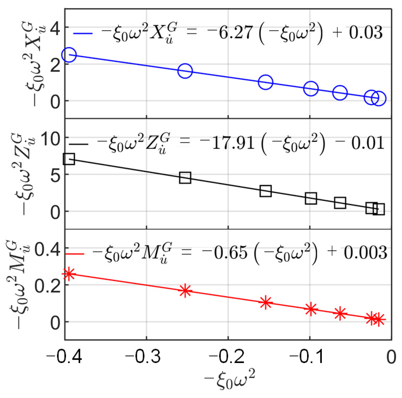
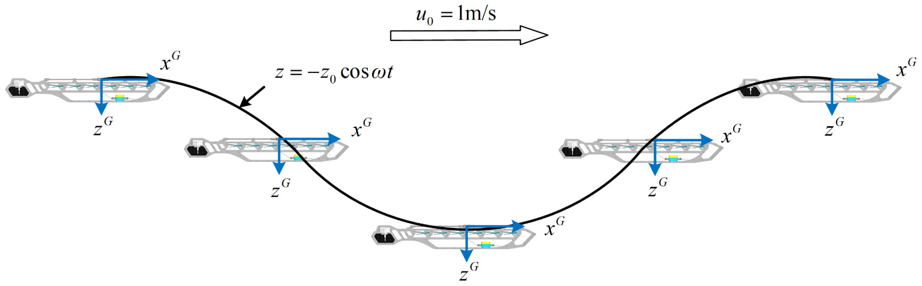
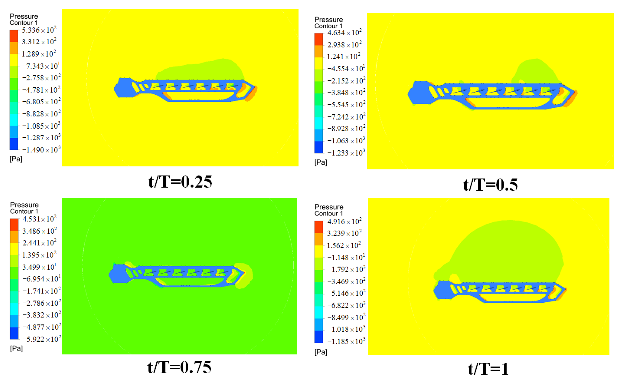
3.3.2. Pure Heave Simulation

In the pure heave simulation, the submerged glider is moving forward at a specified velocity ( u 0 = 1   m / s ) and its x-axis always remains horizontal while the submerged glider is sinusoidally oscillated in the z-direction, which is shown in Figure 12.
The pure heave motion is defined as:
u = u 0 , w = z ˙ , q = 0 u ˙ = 0 , w ˙ = z ¨ , q ˙ = 0 z = z 0 cos ω t
where z , w and w ˙ are the displacement, velocity and acceleration in heave direction, respectively. z 0 is the heave oscillation amplitude. Figure 13 shows the pressure contours of the submerged glider in pure heave simulation when the pitching angle of the hydrofoils is 15 degrees.
Substituting Equation (40) into Equation (37), the hydrodynamic forces and moment acting on the submerged glider can be obtained as:
X H D = X 0 + X w ˙ G z 0 ω 2 cos ω t + X w G z 0 ω sin ω t Z H D = Z 0 + Z w ˙ G z 0 ω 2 cos ω t + Z w G z 0 ω sin ω t + Z | w | w G z 0 2 ω 2 sin ω t M H D = M 0 + M w ˙ G z 0 ω 2 cos ω t + M w G z 0 ω sin ω t + ( X u ˙ G Z w ˙ G ) z 0 ω sin ω t + X w ˙ G ( z 0 ω sin ω t ) 2
Combining all fitting results of pure heave simulation data by the same method, thus the w ˙ dependent added mass coefficients under different pitching angles of the hydrofoils are shown in Figure 14.

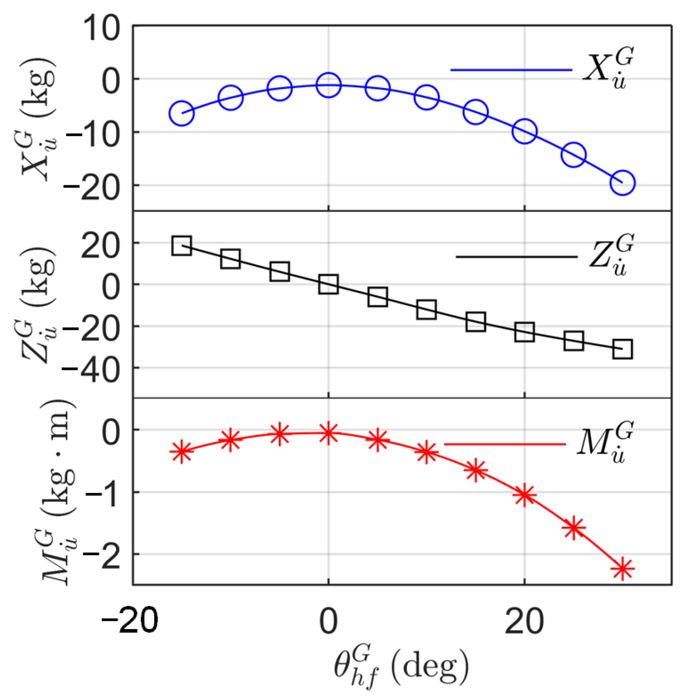
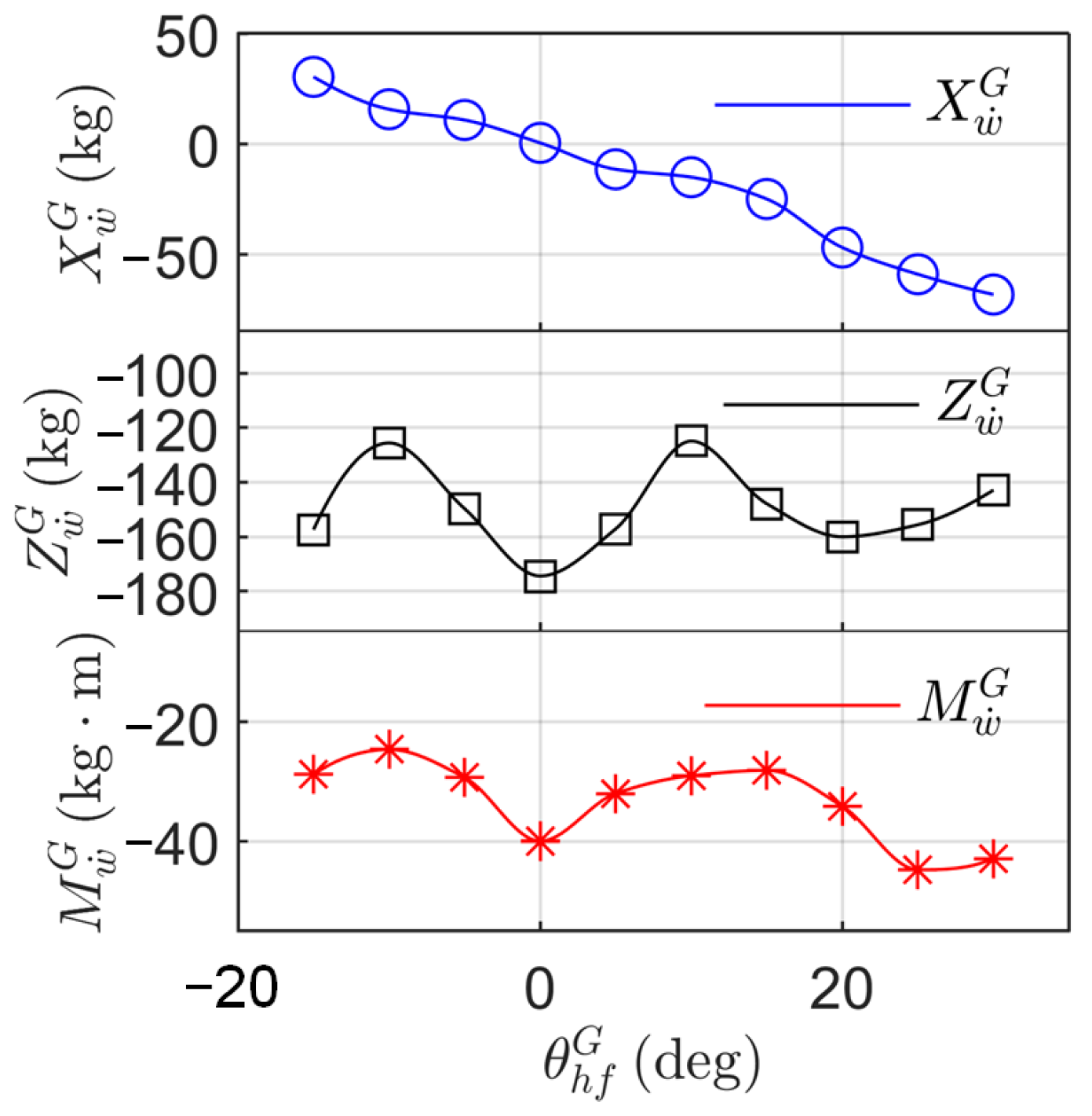
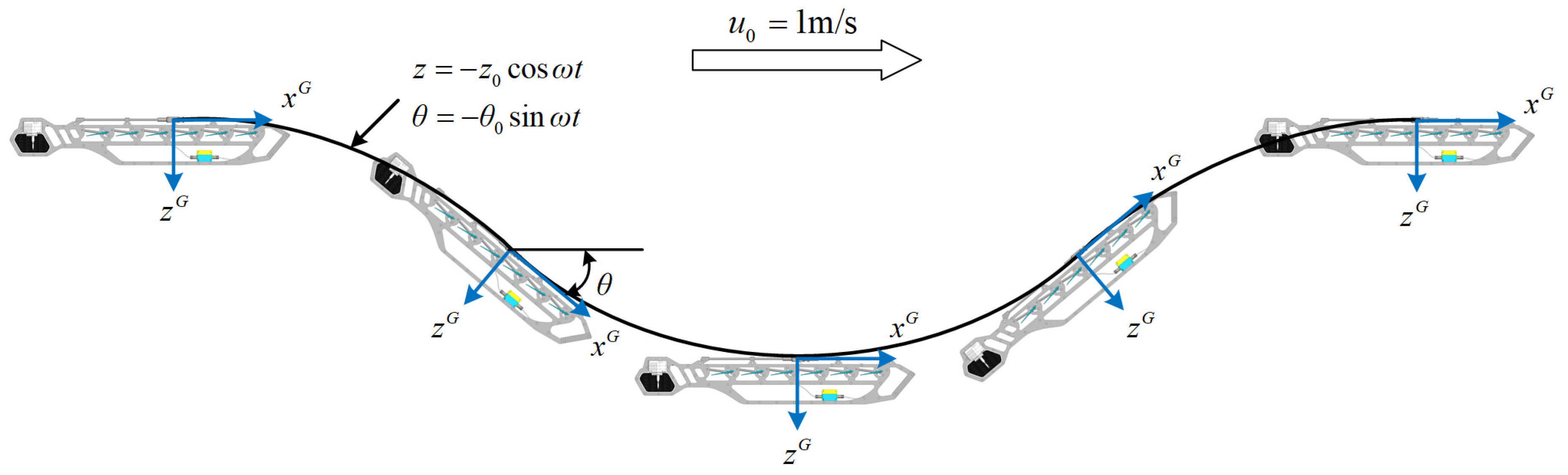
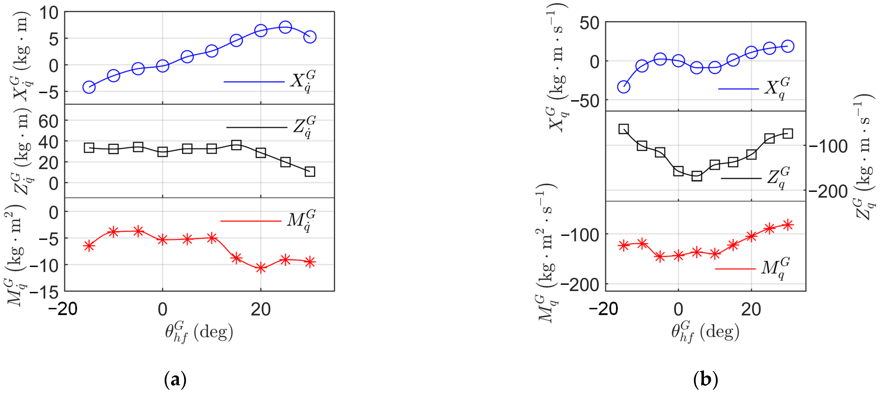
3.3.3. Pure Pitch Simulation

In the pure pitch simulation, the submerged glider moving forward at a specified velocity ( u 0 = 1   m / s ) is sinusoidally oscillated in the z-direction and its x-axis is always tangential to the sinusoidal path, which is shown in Figure 15.
It is intended to obtain q ˙ dependent added mass coefficients and q dependent damping coefficients under different pitching angles of the hydrofoils. The pure pitch motion is defined as:
θ = θ 0 sin ( ω t ) , θ 0 = tan 1 ( z 0 ω u 0 ) u = u 0 cos θ + z ˙ sin θ , u ˙ = z ¨ sin θ θ ˙ ( u 0 sin θ z ˙ cos θ ) w = u 0 sin θ + z ˙ cos θ 0 , w ˙ = z ¨ cos θ θ ˙ ( u 0 cos θ + z ˙ sin θ ) 0 q = θ ˙ , q ˙ = θ ¨
where θ is the pitching angle, q is the pitch angular velocity, q ˙ is the pitch acceleration, u is the surge velocity and u ˙ is the surge acceleration. Figure 16 shows the pressure contours of the submerged glider in pure pitch simulation when the pitching angle of the hydrofoils is 15 degrees.
The hydrodynamic forces and moment acting on the submerged glider can be expressed as:
X H D = X 0 + X q ˙ G q ˙ + X q G q + X u ˙ G u ˙ + Z u ˙ G u q + Z q ˙ G q 2 Z H D = Z 0 + Z q ˙ G q ˙ + Z q G q X u ˙ G u q X q ˙ G q 2 + Z u G u M H D = M 0 + M q ˙ G q ˙ + M q G q Z u ˙ G u 2 Z q ˙ G u q + M u G u
Combining all fitting results of pure pitch simulation data by the same method, the q ˙ dependent added mass coefficients under different pitching angles of the hydrofoils are shown in Figure 17a, and the q dependent added damping coefficient is shown in Figure 17b.

4. Numerical Simulation Validation and Analysis
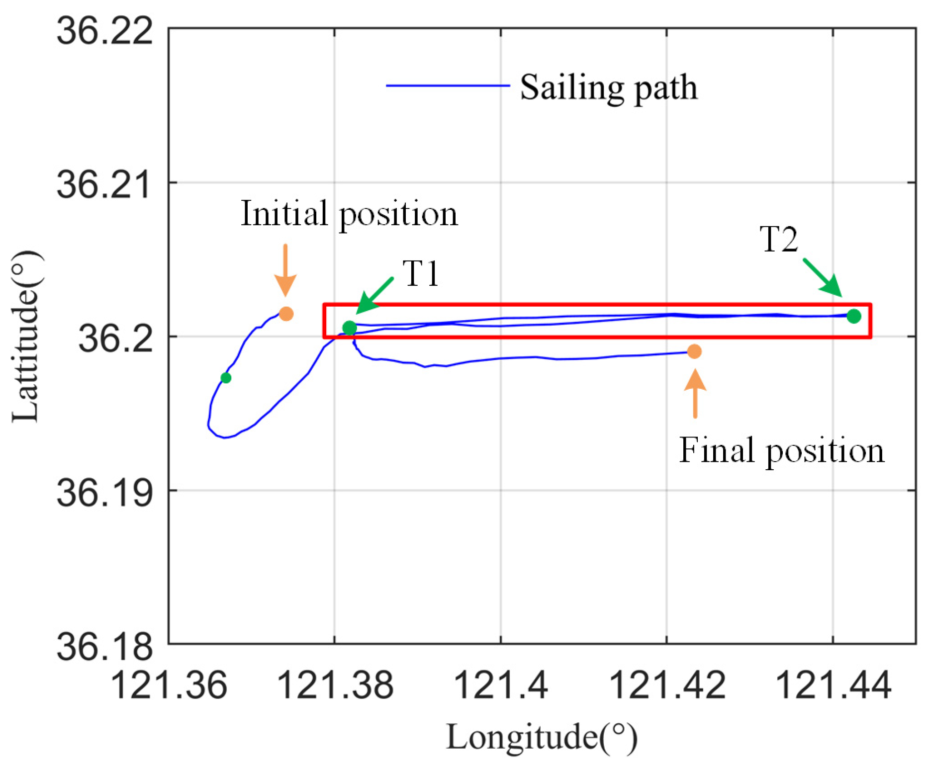
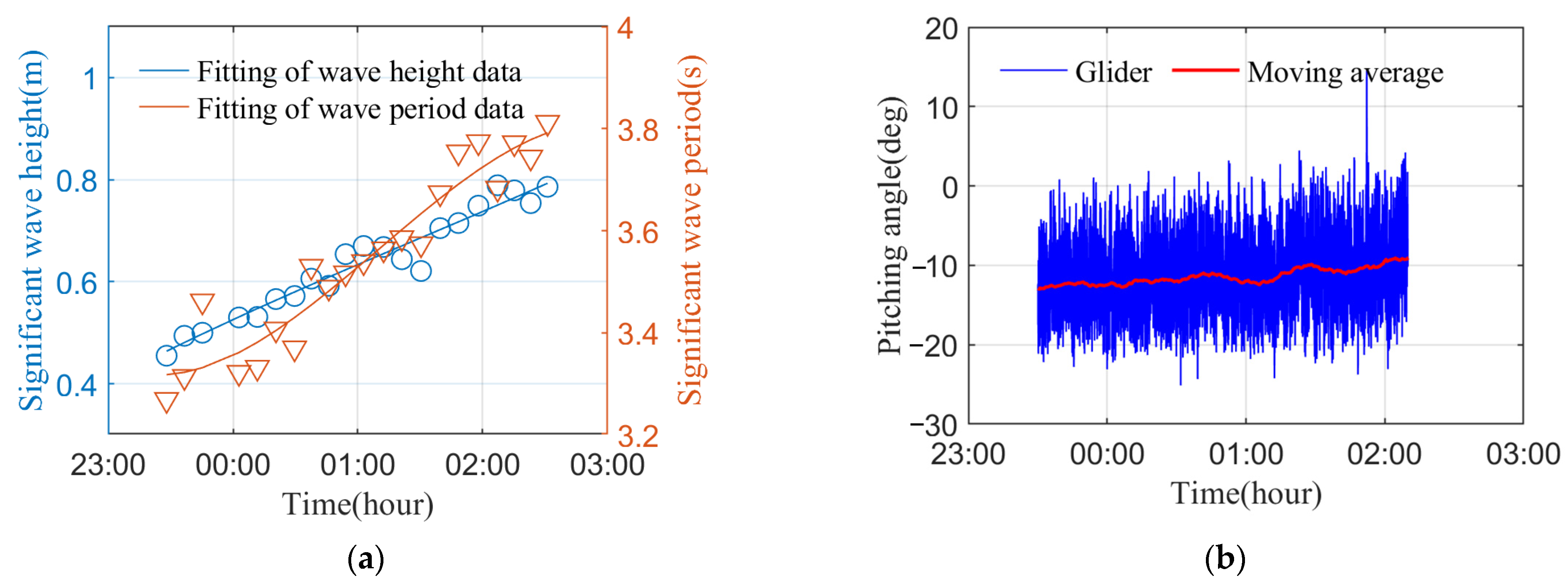
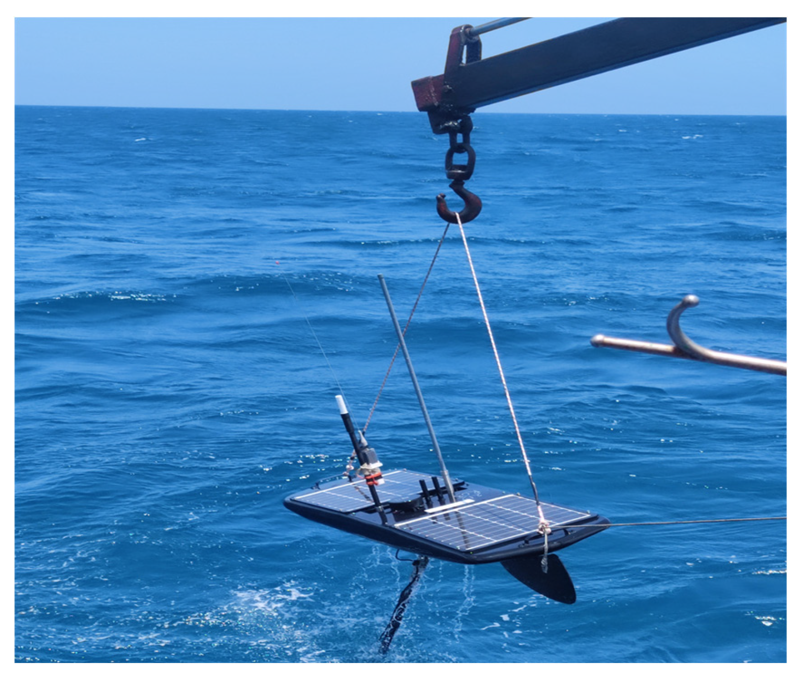
To verify the numerical simulation, simulation results obtained from solution of the dynamic model using the hydrodynamic coefficients are compared with the experimental data in the straight-line paths.
The non-dynamic parameters of the “Black Pearl” wave glider are used in both the sea trial and numerical simulations, which are given in Table 3.

4.1. Sea Trial

In December 2020, sea trial was carried out to test the sailing performance of the “Black Pearl” wave glider, as shown in Figure 18.
Considering the degrees of freedom in the dynamic model, a desired straight-line path between point T1 and point T2 was set. The positions and the velocities of the “Black Pearl” wave glider can be obtained by using a GPS. Figure 19 gives the actual sailing trajectory of the wave glider represented by the blue solid line and the red box is the straight-line path in sea trial. And the red box includes the section of sensor data. In this work, these data were obtained in T 2 T 1 path because the difference between the desired course and the wave direction was relatively stable in this path. The sailing distance from T2 to T1 is about 5.5 km, and the sailing time is about 3 h.
The sea conditions during the sea trial from T2 to T1 were obtained by using a wave sensor; wave data are shown in Figure 20a. Moreover, the real-time values and the moving average value of the pitching angle of the submerged glider are shown in Figure 20b. It can be seen that the average speed of the wave glider increases correspondingly with the continuous increase of significant wave periods and wave heights. Moreover, the average pitching angle and the pitching angle amplitude of the submerged glider both increase slightly.

4.2. Numerical Simulation

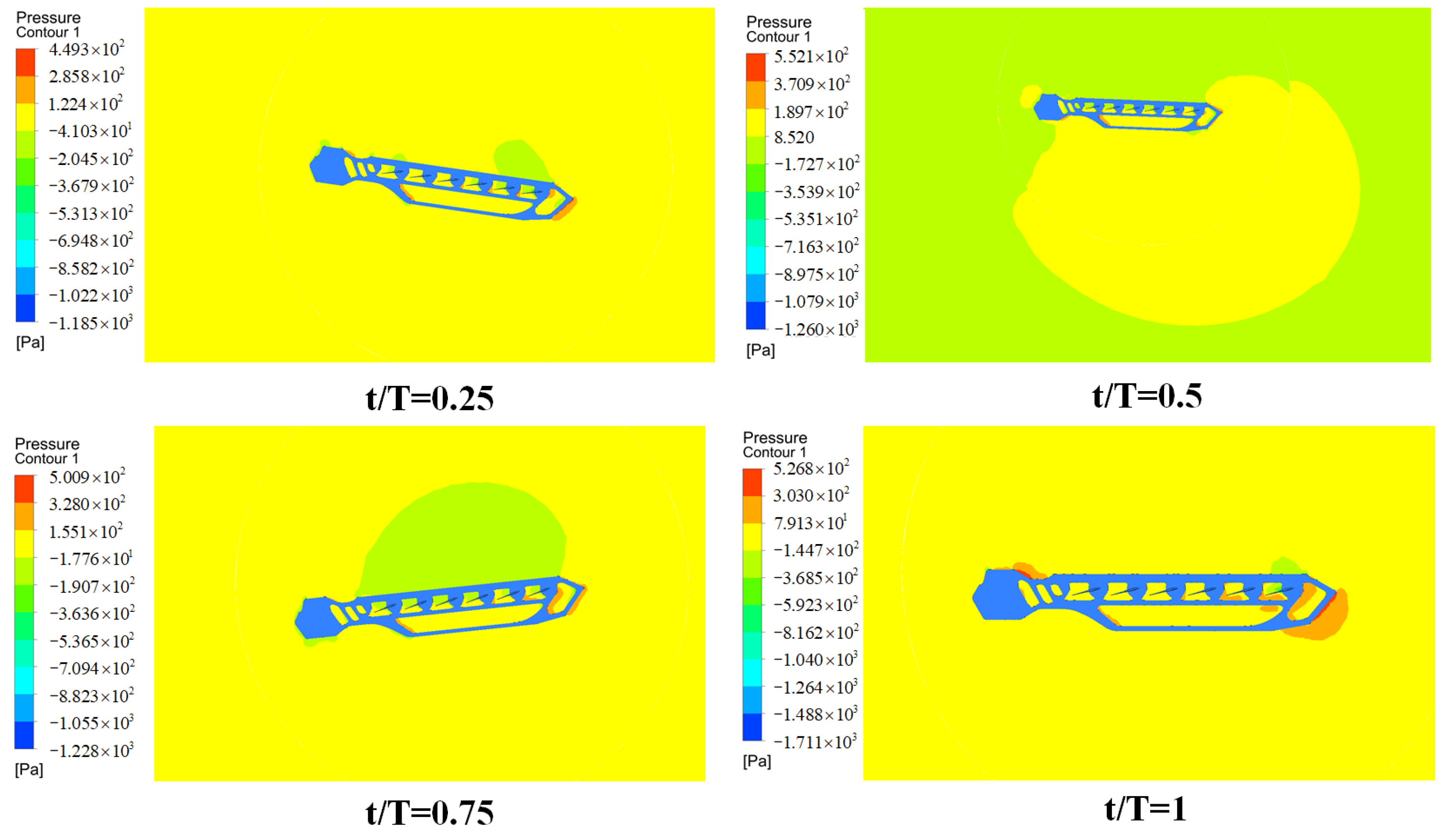
4.2.1. Numerical Simulation with the Specific Sea State

Rampersadh calculated resultant propulsion effect on the float under wave height of 1m and wave period of 10 s [10]. In order to compare with Rampersadh’s calculation results, the dynamic characteristics of the wave glider under the same sea state were examined.
In Figure 21a, the blue, red and blank solid lines, represent the trajectory of the surface float, the trajectory of the submerged glider and the umbilical, respectively. A comparison between Rampersadh’s calculation result and this study’s simulation result is shown in Figure 21b.
Under this specific sea state, the longitudinal average velocities in this study and Rampersadh’s study were, respectively, about 0.41 m/s and 0.4 m/s.

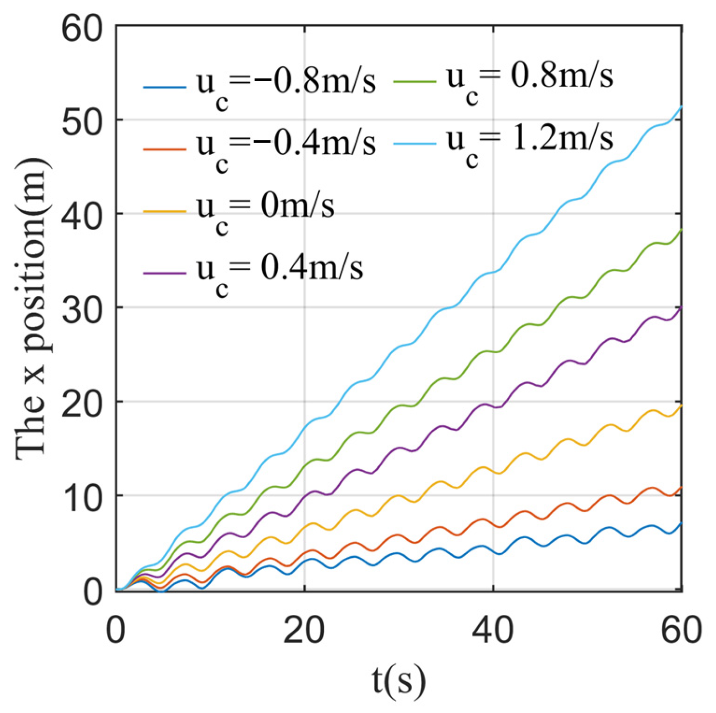
4.2.2. Numerical Simulation Results with Different Current Velocities

The wave height of 0.8 m and the wave period of 4.5 s, which are the average values of experimental data in the sea trial area, are the typical sea state input values of this simulation to analyze the impact of current velocity [37]. Figure 22 shows the positions of the surface float in the ξ direction under different current velocities and the same sea state.
As seen in Figure 22, the positive current velocity is conducive to improving the navigation velocity of the wave glider, but the negative current velocity will reduce the navigation performance of the wave glider, reflecting the bigger hydrodynamic damping. In addition, the greater the positive or negative current velocity, the greater the favorable or hindering effect on the navigation performance of the wave glider.

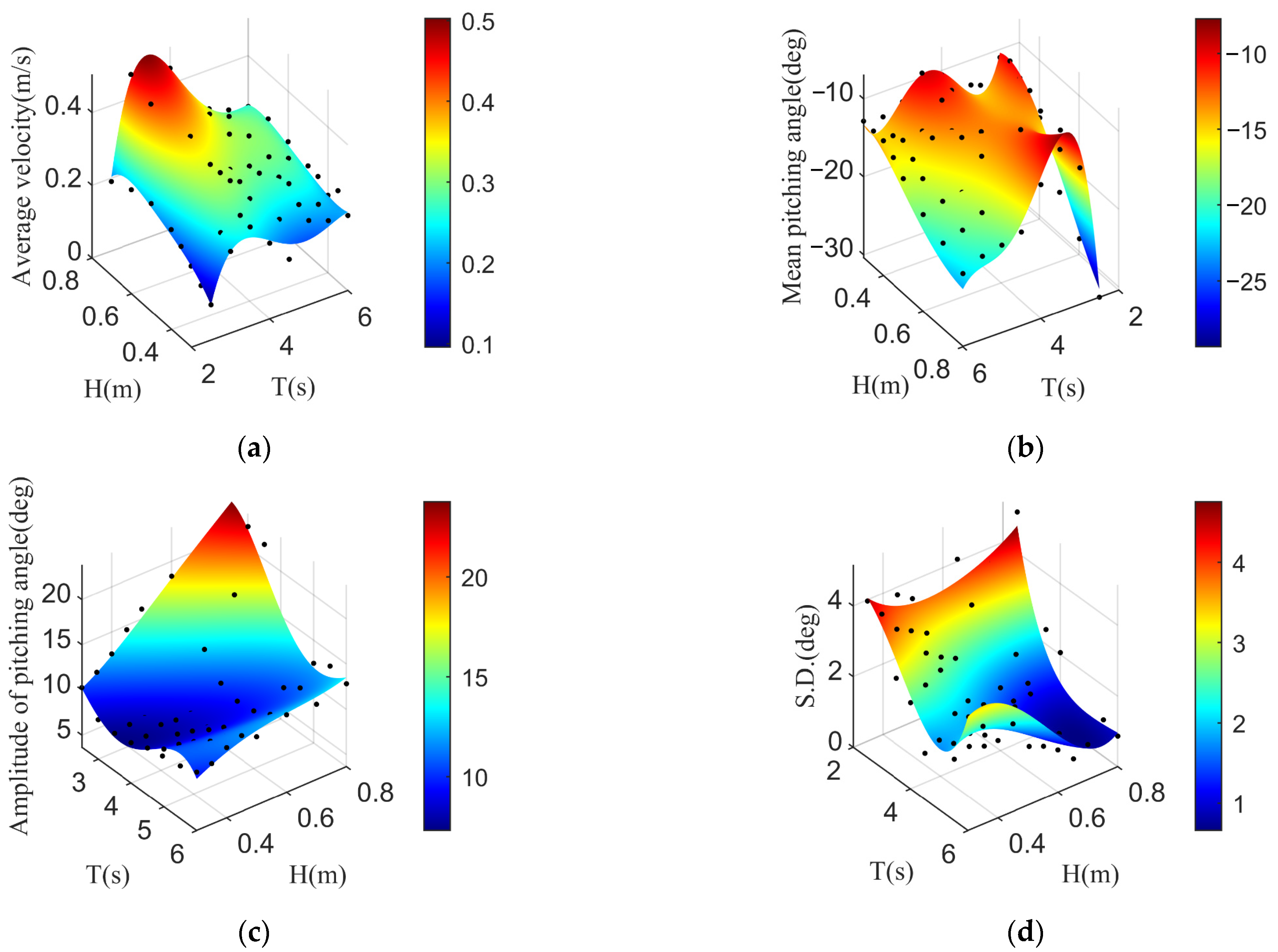
4.2.3. Numerical Simulation Results with the Different Sea States

To study the effects of wave height and wave period on sailing performance of the submerged glider, the simulated sea states through a two-by-two combination of wave height and wave period are given in Table 4. Due to the complexity and variability of the marine environment, the interaction between the surface float and wave was simplified. The initial speeds of the surface float and the submerged glider and the initial pitching angle of the umbilical were all set to 0. The initial pitching angles of the submerged glider and the hydrofoils were set by calculating coupled hydrostatics of the submerged glider and the hydrofoils. The actual current velocity in the sea trial is unknown because the ADCP is not carried on the surface float. Thus, the current velocity in simulations is set to 0.
Numerical simulation results for longitudinal motion under different sea states are shown in Figure 23.
Figure 23a gives the longitudinal average velocities of the wave glider under different sea states. In general, a high wave height with the same wave period is favorable for the forward sailing performance of the wave glider.
The average pitching angle and the pitching angle amplitude of the submerged glider are shown in Figure 23b,c, respectively. It can be seen from Figure 23b that the average pitching angle of the submerged glider almost maintained between 15 degrees and 20 degrees when the sea states were the same as the sea trial data. Moreover, the average pitching angle for the high wave height changes significantly in different wave periods.
In addition, it can be seen from Figure 23c that the high wave period is beneficial to reduce the pitch amplitude, especially for the high wave height. Moreover, the low wave height with the same wave period is conducive to decreasing the pitching angle amplitude of the submerged glider.
Figure 23d presents the standard deviation of the pitching angle of the submerged glider under different sea states, which describes the deviation magnitude of the centerline of the pitching angle from its average value. The low wave period is the main factor leading to the increase of the standard deviation.
Furthermore, the forward sailing performance of the wave glider is sensitive to wave period, especially in a high wave height with a low wave period. It can be seen from Figure 23b,c that under a high wave height with a low wave period, the average value, the amplitude and the standard deviation of the pitching angle suddenly change. Therefore, it means that the submerged glider is in an unstable state, which will lead to a significant reduction in the longitudinal average velocity.

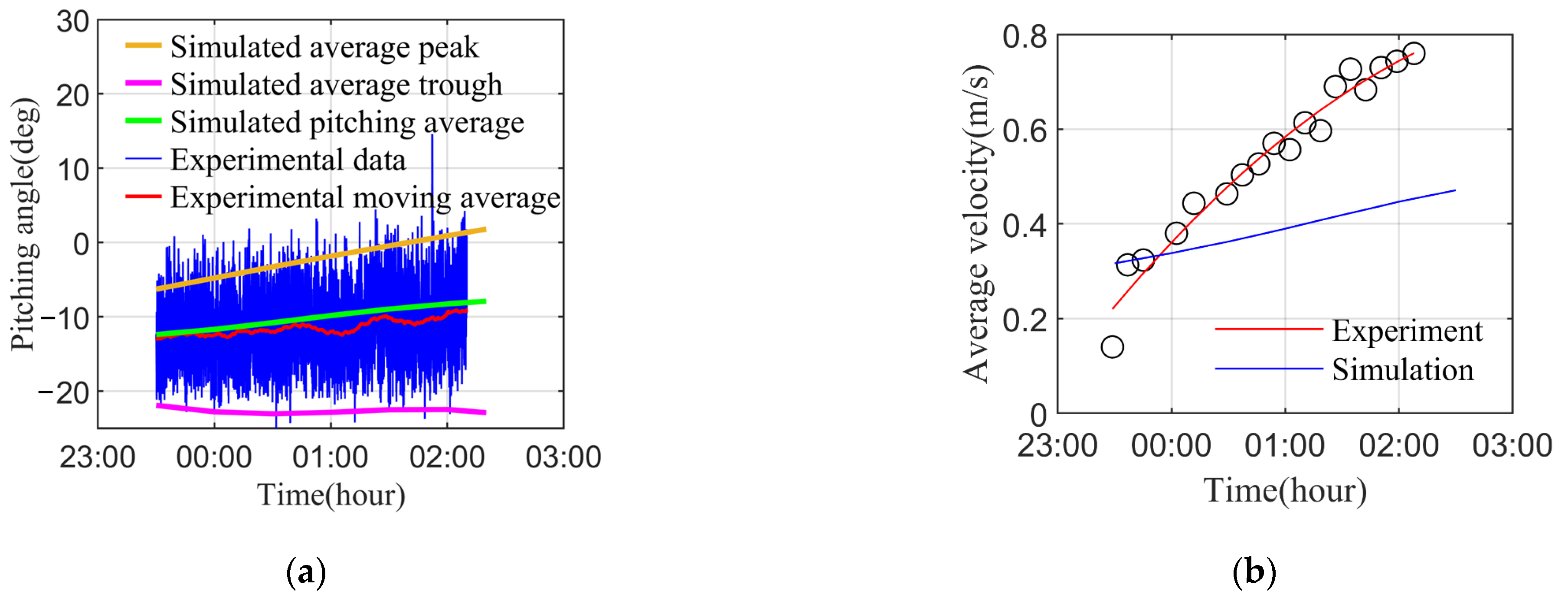
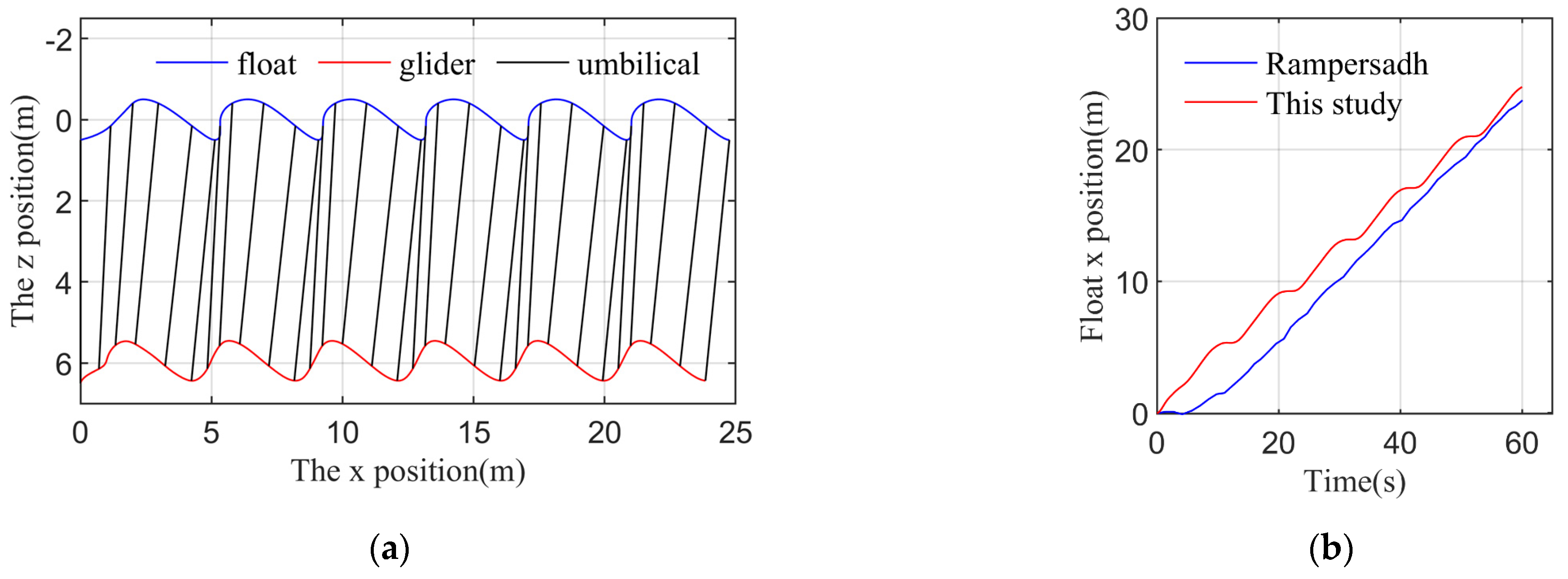
4.3. Numerical Simulation Validation

Numerical simulations were performed to compare the average velocity of the wave glider, the amplitude and the moving average of the pitching angles of the submerged glider with sea trial data. To verify the effectiveness of the numerical simulation, sea states obtained every 15 minutes are used as input conditions for simulations.
The trends of simulated average pitching angles, average peaks, average troughs, and average velocities are shown in Figure 24a, which is similar with experimental data.
It can be seen from Figure 24a that simulated average peaks are consistent with the first half of experimental data, but it exists gradually, with increasing upward-offset compared with the other of experimental data. In the first half, the estimated average difference between simulated pitching average and the moving average of the pitching angle of experimental data is about one degree, which is small. However, in the latter part, it is approximately twice the average difference than that of the first half, and the maximum difference is about three degrees. In addition, the downward-offset of simulated average troughs relative to experimental data is about 5 degrees. It can be seen from Figure 24b that simulated longitudinal average velocity is in the upward trend with the same as experimental velocity, but the increasing trend is slower than that of experimental velocity.
In the above comparison, it is acceptable in engineering practice to have a certain degree of error between the simulated data and experimental data. The reason for this is that the assumptions used in the numerical simulation are simplifications of the actual conditions. For example, the winds and the ocean currents are ignored, and actual wave conditions are constantly changing, but wave conditions in simulations are constant.

5. Conclusions

In this paper, to improve the propulsion performance of the wave glider, a 4-DOF dynamic model of the wave glider based on the dynamic characteristics of the tandem hydrofoils is built. The unknown hydrodynamic coefficients in the dynamic model are obtained. The “Black Pearl” wave glider is adopted for the sea trial, and straight-line path is set to verify the numerical simulation. The propulsion performance of the wave glider is compared in simulation in terms of wave parameters, the velocities and some pitching angles of the wave glider. Some conclusions can be drawn as follows:
(1)
The proposed model and the numerical simulation using those hydrodynamic coefficients are found to be reasonable and acceptable in practice by comparison with the experimental data;
(2)
The numerical simulation can predict the longitudinal velocity of the wave glider and the pitching angle of the submerged glider and analyze the stability of the submerged glider from the mean value, the amplitude and the standard deviation of the pitching angle;
(3)
Under the same sea state, the positive current velocity is conducive to improving the navigation velocity of the wave glider, but the negative current velocity will reduce the navigation performance of the wave glider, reflecting the bigger hydrodynamic damping. In addition, the greater the positive or negative current velocity, the greater the favorable or hindering effect on the navigation performance of the wave glider;
(4)
The wave height and the wave period are the main factors affecting the straight-line sailing performance of the wave glider. Furthermore, the pitching stability of the submerged glider is also crucial for the wave glider to converse the energy obtained from ocean waves into the forward thrust.
In future research, ocean current velocity will be taken into account in dynamical models. Moreover, the influences of the complex ocean environment on wave gliders will also be considered to be closer to the realistic environment; for example, the wave loads and the motion responses of the surface float under irregular waves and different wave incident angles.

Author Contributions

Conceptualization, resources, X.S.; methodology, analysis, writing–original draft, C.S.; methodology, writing–review and editing, H.S.; sea trial, analysis, C.L. All authors have read and agreed to the published version of the manuscript.

Funding

This research is supported by the National Key Research and Development Program of China (No. SQ2020YFF0426588), the Major Scientific and Technological Innovation Projects of Shandong Province (No.2019JZZY020701), the National Key Research and Development Plan of China (No.2017YFC0305902), and the Wenhai Program of Qingdao National Laboratory for Marine Science and Technology (No.2017WHZZB0101).

Institutional Review Board Statement

Not applicable.

Informed Consent Statement

Not applicable.

Data Availability Statement

Not applicable.

Acknowledgments

The authors appreciate all staff members in research and development team of the “Black Pearl” wave gliders.

Conflicts of Interest

The authors declare no conflict of interest.

References

  1. Hine, R.; Willcox, S.; Hine, G.; Richardson, T. The Wave Glider: A Wave-Powered autonomous marine vehicle. In Proceedings of the OCEANS 2009, Biloxi, MS, USA, 26–29 October 2009; IEEE: New York, NY, USA, 2010; pp. 1–6. [Google Scholar]
  2. Liu, P.; Su, Y.M.; Liao, Y.L. Numerical and experimental studies on the propulsion performance of a Wave Glide propulsor. China Ocean Eng. 2016, 30, 393–406. [Google Scholar] [CrossRef]
  3. Qi, Z.; Zou, B.; Lu, H.; Shi, J.; Li, G.; Qin, Y.; Zhai, J. Numerical investigation of the semi-active flapping foil of the wave glider. J. Mar. Sci. Eng. 2020, 8, 13. [Google Scholar] [CrossRef] [Green Version]
  4. Yang, F.; Shi, W.; Wang, D. Systematic study on propulsive performance of tandem hydrofoils for a wave glider. Ocean Eng. 2019, 179, 361–370. [Google Scholar] [CrossRef] [Green Version]
  5. Yang, F.; Shi, W.; Zhou, X.; Guo, B.; Wang, D. Numerical investigation of a wave glider in head seas. Ocean Eng. 2018, 164, 127–138. [Google Scholar] [CrossRef] [Green Version]
  6. Kraus, N.; Bingham, B. Estimation of wave glider dynamics for precise positioning. In Proceedings of the OCEANS’11 MTS/IEEE KONA, Waikoloa, HI, USA, 19–22 September 2011; IEEE: New York, NY, USA, 2011; pp. 1–9. [Google Scholar]
  7. Kraus, N.D. Wave Glider Dynamic Modeling, Parameter Identification and Simulation. Master’s Thesis, University of Hawaii, Honolulu, HI, USA, 2012. [Google Scholar]
  8. Qi, Z.F.; Liu, W.X.; Jia, L.J.; Qin, Y.F.; Sun, X.J. Dynamic modeling and motion simulation for wave glider. Appl. Mech. Mater. 2013, 397–400, 285–290. [Google Scholar] [CrossRef]
  9. Li, X.T.; Liu, F.; Wang, L.; She, H.Q. Motion analysis of wave glider based on multibody dynamic theory. In Proceedings of the 10th International Conference on Intelligent Robotics and Applications, ICIRA, Wuhan, China, 16–18 August 2017; Springer: Cham, Switzerland; pp. 721–734. [Google Scholar]
  10. Rampersadh, G. Sea-State Interaction Based Dynamic Model of the Liquid Robotics’ Wave Glider: Modelling and Control of a Hybrid Multi-Body Vessel. Master’s Thesis, University of Cape Town, Cape Town, South Africa, 2018. [Google Scholar]
  11. Wang, P.; Tian, X.L.; Lu, W.Y.; Hu, Z.H.; Luo, Y. Dynamic modeling and simulations of the wave glider. Appl. Math. Model. 2019, 66, 77–96. [Google Scholar] [CrossRef]
  12. Chen, J.; Ge, Y.; Yao, C.; Zheng, B. Dynamics Modeling of a Wave Glider with Optimal Wing Structure. IEEE Access 2018, 6, 71555–71565. [Google Scholar] [CrossRef]
  13. Wang, L.; Li, Y.; Liao, Y.; Pan, K.; Zhang, W. Dynamics modeling of an unmanned wave glider with flexible umbilical. Ocean Eng. 2019, 180, 267–278. [Google Scholar] [CrossRef]
  14. Slone, A.K.; Pericleous, K.; Bailey, C.; Cross, M. Dynamic fluid–structure interaction using finite volume unstructured mesh procedures. Comput. Struct. 2002, 80, 371–390. [Google Scholar] [CrossRef]
  15. Westphalen, J.; Greaves, D.M.; Raby, A.; Hu, Z.Z.; Causon, D.M.; Mingham, C.G.; Omidvar, P.; Stansby, P.K.; Rogers, B.D. Investigation of Wave-Structure Interaction Using State of the Art CFD Techniques. Open J. Fluid Dyn. 2014, 4, 18–43. [Google Scholar] [CrossRef] [Green Version]
  16. Ren, B.; Jin, Z.; Gao, R.; Wang, Y.X.; Xu, Z.L. SPH-DEM modeling of the hydraulic stability of 2D blocks on a slope. J. Waterw. Port Coast. Ocean Eng. 2014, 140, 04014022. [Google Scholar] [CrossRef]
  17. Xiang, T.; Istrati, D.; Yim, S.C.; Buckle, I.G.; Lomonaco, P. Tsunami Loads on a Representative Coastal Bridge Deck: Experimental Study and Validation of Design Equations. J. Waterw. Port Coast. Ocean. Eng. 2020, 146, 04020022. [Google Scholar] [CrossRef]
  18. Hasanpour, A.; Istrati, D.; Buckle, I. Coupled SPH–FEM Modeling of Tsunami-Borne Large Debris Flow and Impact on Coastal Structures. J. Mar. Sci. Eng. 2021, 9, 1068. [Google Scholar] [CrossRef]
  19. Zhang, H.; Xu, Y.R.; Cai, H.P. Using CFD software to calculate hydrodynamic coefficients. J. Mar. Sci. Appl. 2010, 9, 149–155. [Google Scholar] [CrossRef]
  20. Malik, S.A.; Guang, P. Transient numerical simulations for hydrodynamic derivatives predictions of an axisymmetric submersible vehicle. Res. J. Appl. Sci. Eng. Technol. 2013, 5, 5003–5011. [Google Scholar] [CrossRef]
  21. Can, M. Numerical Simulation of Hydrodynamic Planar Motion Mechanism Test for Underwater Vehicles. Master’s Thesis, Middle East Technical University, Ankara, Turkey, 2014. [Google Scholar]
  22. Singh, Y.; Bhattacharyya, S.K.; Idichandy, V.G. CFD approach to modelling, hydrodynamic analysis and motion characteristics of a laboratory underwater glider with experimental results. J. Ocean Eng. Sci. 2017, 2, 90–119. [Google Scholar] [CrossRef]
  23. Xiang, T.; Istrati, D. Assessment of Extreme Wave Impact on Coastal Decks with Different Geometries via the Arbitrary Lagrangian-Eulerian Method. J. Mar. Sci. Eng. 2021, 9, 1342. [Google Scholar] [CrossRef]
  24. Rudmana, M.; Cleary, P.W. Oblique impact of rogue waves on a floating platform. In Proceedings of the International Ocean and Polar Engineering Conference 2009, Osaka, Japan, 21–26 June 2009; The International Society of Offshore and Polar Engineers: Mountain View, CA, USA, 2009; pp. 572–579. [Google Scholar]
  25. Peregrine, D.H.; Bredmose, H.; Bullock, G.; Obrhai, C.; Muller, G.; Wolters, G. Water wave impact on walls and the role of air. In Proceedings of the Coastal Engineering 2004, Lisbon, Portugal, 19–24 September 2004; World Scientific: Hackensack, NJ, USA, 2005; pp. 4005–4017. [Google Scholar]
  26. Ghosh, S.; Reins, G.; Koo, B.; Wang, Z.; Yang, J.; Stern, F. Plunging wave breaking: EFD and CFD. In Proceedings of the International Conference on Violent Flows, Fukuoka, Japan, 20–22 November 2007; National University: Fukuoka, Japan, 2007. [Google Scholar]
  27. Istrati, D. Large-Scale Experiments of Tsunami Inundation of Bridges including Fluid-Structure-Interaction. Ph.D. Thesis, University of Nevada, Reno, NV, USA, 2017. [Google Scholar]
  28. Leschka, S.; Oumeraci, H. Solitary waves and bores passing three cylinders-effect of distance and arrangement. Coast. Eng. 2014, 1, 39. [Google Scholar] [CrossRef] [Green Version]
  29. Istrati, D.; Buckle, I.; Lomonaco, P.; Yim, S. Deciphering the Tsunami Wave Impact and Associated Connection Forces in Open-Girder Coastal Bridges. J. Mar. Sci. Eng. 2018, 6, 148. [Google Scholar] [CrossRef] [Green Version]
  30. Fossen, T.I. Handbook of Marine Craft Hydrodynamics and Motion Control, 1st ed.; John Wiley & Sons, Ltd.: Chichester, UK, 2011. [Google Scholar]
  31. Jakuba, M.V. Modeling and Control of an Autonomous Underwater Vehicle with Combined Foil/Thruster Actuators. Master’s Thesis, Massachusetts Institute of Technology, Cambridge, MA, USA, 2003. [Google Scholar]
  32. Wilcox, D.C. Turbulence Modeling for CFD; DCW Industries Inc.: La Canada, CA, USA, 2006. [Google Scholar]
  33. Celik, I.B.; Ghia, U.; Roache, P.J.; Freitas, C.J.; Coleman, H.; Raad, P.E. Procedure for estimation and reporting of uncertainty due to discretization in CFD applications. J. Fluid Eng. Trans. ASME 2008, 130, 078001–078004. [Google Scholar]
  34. Park, J.Y.; Kim, N.; Shin, Y.K. Experimental study on hydrodynamic coefficients for high-incidence-angle maneuver of a submarine. Int. J. Nav. Archit. Ocean Eng. 2017, 9, 100–113. [Google Scholar] [CrossRef] [Green Version]
  35. Watt, G.D. Modelling and Simulating Unsteady Six Degrees-of-Freedom Submarine Rising Maneuvers; DRDC Atlantic TR 2007-008; Defence Research and Development Canada: Ottawa, ON, Canada, 2007. [Google Scholar]
  36. Coe, R.G.; Neu, W.L. Amplitude effects on virtual PMM tests. In Proceedings of the 2012 Oceans, Hampton Roads, VA, USA, 26–29 October 2012; IEEE: New York, NY, USA, 2013; pp. 1–5. [Google Scholar]
  37. Li, C. Dynamics Analysis and Performance Optimization of the Wave Glider. Master’s Thesis, Tiangong University, Tianjin, China, 2018. (In Chinese). [Google Scholar]
Figure 1. The working principle of the wave glider.
Jmse 10 00520 g001
Figure 2. The coordinate frames of the “Black Pearl” wave glider.
Jmse 10 00520 g002
Figure 3. The vectors of drag force, lift force and flow velocity.
Jmse 10 00520 g003
Figure 4. The force diagram of the hydrofoil.
Jmse 10 00520 g004
Figure 5. The XOZ section of the computational domain.
Jmse 10 00520 g005
Figure 6. Simulation cases of static tests.
Jmse 10 00520 g006
Figure 7. The simulation and fitting results of static tests: (a) surge force; (b) heave force; (c) pitch moment.
Jmse 10 00520 g007
Figure 8. The schematic diagram of the pure surge test.
Jmse 10 00520 g008
Figure 9. The pressure contours of the submerged glider in pure surge simulation ( θ h f G = 15 ° ).
Jmse 10 00520 g009
Figure 10. Simulation and fitting results ( θ h f G = 15 ° ).
Jmse 10 00520 g010
Figure 11. The results of u ˙ dependent added mass coefficients.
Jmse 10 00520 g011
Figure 12. The schematic diagram of the pure heave test.
Jmse 10 00520 g012
Figure 13. The pressure contours of the submerged glider in pure heave simulation ( θ h f G = 15 ° ).
Jmse 10 00520 g013
Figure 14. The results of w ˙ dependent added mass coefficients.
Jmse 10 00520 g014
Figure 15. The schematic diagram of the pure pitch test.
Jmse 10 00520 g015
Figure 16. The pressure contours of the submerged glider in pure pitch simulation ( θ h f G = 15 ° ).
Jmse 10 00520 g016
Figure 17. The results of pure pitch simulation: (a) the results of q ˙ dependent added mass coefficients; (b) the results of q dependent added damping coefficients.
Jmse 10 00520 g017
Figure 18. The “Black Pearl” wave glider in sea trial.
Jmse 10 00520 g018
Figure 19. The trajectory of the wave glider.
Jmse 10 00520 g019
Figure 20. Experimental data in the sea trial: (a) varying significant wave heights and wave periods; (b) the pitching angle of the submerged glider.
Jmse 10 00520 g020
Figure 21. Simulation results with the specific sea state. (a) The x-z view of the wave glider; (b) comparison result.
Jmse 10 00520 g021
Figure 22. Comparison of the position of the surface float under different current velocities.
Jmse 10 00520 g022
Figure 23. Numerical simulation results for longitudinal motion under different sea states, the black dots are numerical simulation data, and the continuous colorful planes are generated after interpolation about numerical simulation data: (a) the longitudinal average velocities of the wave glider; (b) the mean pitching angles of the submerged glider; (c) the pitching angle amplitude of the submerged glider; (d) the standard deviation of the pitching angle.
Jmse 10 00520 g023
Figure 24. Numerical simulation results comparing with experimental data. (a) The simulated pitching angles comparing with experimental data; (b) the simulated longitudinal average velocities of the wave glider comparing with experimental data.
Jmse 10 00520 g024
Table 1. Average grid sizes of different zones.
ValueUnit
Inner zone 8.2 × 10 6 m3
Middle zone 6.7 × 10 3 m3
Outer zone 8 × 10 3 m3
Table 2. Grid convergence analysis.
Axial ForceVertical ForcePitch Moment
Output values ϕ 1 −34.094116.55221.503
ϕ 2 −34.116116.48421.602
ϕ 3 −34.142116.51321.681
Refinement ratio r 21 1.342
r 32 1.358
Order of accuracy p 0.42272.98290.9229
GCI GCI 21 0.00610.000520.018
GCI 32 0.00690.000210.014
Table 3. Non-dynamic parameters of the “Black Pearl” wave glider.
ParameterDescriptionValueUnit
m F Mass of the surface float27.5kg
m G Mass of the submerged glider30kg
m h f Mass of a pair of tandem hydrofoils2.137kg
M q ˙ h f Pitching added mass of a pair of tandem hydrofoils0.3734kg∙m2
B h f Buoyancy of a pair of tandem hydrofoils11.065N
D f l o a t Surface float dimension1.8 × 0.5 × 0.2m3
D g l i d e r Submerged glider dimension1.9 × 1.1 × 0.3m3
L u m b Initial length of the umbilical6m
g Gravity constant9.81m/s2
Table 4. Sea states for numerical simulation.
Wave Height (m)Wave Period (s)
0.32.5
0.353
0.43.5
0.454
0.54.5
0.65
0.75.5
0.86
Publisher’s Note: MDPI stays neutral with regard to jurisdictional claims in published maps and institutional affiliations.

