Meaningful Trend in Climate Time Series: A Discussion Based On Linear and Smoothing Techniques for Drought Analysis in Taiwan

Abstract

Finding significant trends in hydroclimate time series has been deemed an essential task in numerous studies. Despite the existence of various trend detection methods, statistical significance is mostly examined for linear trends and related to the meaningfulness of the found trends. We wish to draw attention to a more general definition of meaningful trends by cross-referencing not only linear but also smoothing techniques. We apply linear regression (LR) and two smoothing techniques based on regularized minimal-energy tensor-product B-splines (RMTB) to the trend detection of standardized precipitation index (SPI) series over Taiwan. LR and both RMTB-based methods identify an overall upward (wetting) trend in the SPI series across the time scales in Taiwan from 1960 to 2019. However, if dividing the entire time series into the earlier (1960–1989) and later (1990–2019) sub-series, we find that some downward (drying) trends at varied time scales migrate from southcentral–southwestern to eastern regions. Among these significant trends, we have more confidence in the recent drying trend over eastern Taiwan since all the methods show trend patterns in highest similarity. We also argue that LR should be used with great caution, unless linearity in data series and independence and normality in residuals can be assured.

1. Introduction

Global warming, regardless of the contribution from human activities or natural causes, has intensified hydroclimate variability [1]. More extreme events (e.g., floods, droughts, and storms) that only take place at certain timestamps in history could be significant enough to determine the variability or “direction” of long-term climate time series; this is perhaps a more discernible condition than a gradual change in the records. To unravel the characteristics of climate conditions varying over time, trend analysis commonly adopted in many scientific disciplines has come into play. In the field of meteorology and climate sciences, trend analysis actually has already exhibited various applications, including the understanding of temporal patterns of hydroclimatic variables (e.g., precipitation, temperature, and streamflow) subject to climate change [2] and land use/cover change [3]. Results from trend analysis could also be incorporated in the development of climate adaptation strategies [4].

The proliferation of studies on climate variability analysis has incubated various trend or change-point detection methods. Some of the most classical methods, either parametric or nonparametric, include least squares linear regression, the Mann–Kendall (MK) test [5], Theil–Sen (or Sen’s) slope estimators [6,7], the Pettitt test [8], etc. Even though these methods have a long history, they are still being applied to numerous recent hydroclimate-related studies. For instance, lref. [4] applied the MK test to examine trends in precipitation and temperature at yearly, seasonal, and monthly time scales over the northwestern region of Bangladesh from 1980–2008; they indicated that their trend analysis results should be important to the planning of climate adaptation strategies in preparation for future climate conditions. Ref. [9] lproposed a framework that quantifies how climate change and human activities influence hydrological drought; in their framework, they used the MK and Pettitt tests to examine trend and change points in hydrological variable series (e.g., precipitation, potential evapotranspiration, and runoff) over a semiarid basin in northern China Ref. [10] evaluated trend and change points in annual and seasonal rainfall series using the MK and Pettitt tests in the Niger Central Hydrological Area; they also derived the rainfall variability index and precipitation concentration index for a better illustration of rainfall variability. Apart from these classical methods, some new methods for trend detection have been developed as well: ref. [11] developed and used the innovative trend analysis method in conjunction with the MK test and Sen’s slope estimate for trend analysis on rainfall in the Upper Wabe Shebelle River Basin in Ethiopia.

The above references have shown that using multiple trend detection methods in one study is a common practice. The rationale behind it is to account for uncertainty in trend detection results due to different assumptions and mechanisms used, yet a reasonable interpretation of the discrepancy in trends (both direction and significance) is usually a challenging, easily forgotten issue to address. In fact, it might be human nature to emphasize more on trend with significance and less on trend with no significance or discrepancy. We however, argue that the discrepancy or similarity between trend detection results should be a useful indicator of the existence of real or “meaningful” trend.

In Taiwan, studies related to hydroclimatic trend or change-point analysis are also abundant. Ref. [12] applied the Pettitt test to the detection of change points in the standardized precipitation index (SPI) at a three-monthly time scale, and found that meteorological drought has decreased (increased) in northeastern (central and southern) Taiwan since the 1960s. Ref. [13] applied the MK test, Sen’s slope estimator, and the Pettitt test to the analysis of trends and change points in annual rainfall, temperature, and groundwater level series, in order to assess groundwater resource subject to excessive pumping in southwestern Taiwan. Another drought study by [14] also employed the SPI jointly with the streamflow drought index (SDI) to assess the trends and characteristics of drought in southern Taiwan; the results based on the MK test and Theil–Sen slope estimators revealed that although there exists an overall increasing trend in the SPI (i.e., more rainfall, thus milder meteorological droughts in recent years), at some stations a significant decreasing trend in the SDI (i.e., more hydrological droughts) can be found. Ref. [15] extended the scope of drought analysis in Taiwan to the future using the downscaled data from 26 sets of global climate model projections; they showed that the frequency of short-term drought events (3-month SPI) would increase by the end of 21st century. In contrast to drought analysis, ref. [16] employed linear regression (LR), the MK test, and Theil–Sen slope estimator to analyze Taiwan’s extreme rainfall derived from a recently released gridded rainfall dataset; they found an increasing trend in island-wide extreme rainfall, most significant in the winter, spring, and typhoon seasons. According to our literature review of hydroclimatic trend analysis for Taiwan, we note that most of them are only station-based or regional assessments using classical trend detection techniques. We believe that a national assessment using gridded data (as used in [16]) and emerging trend detection techniques, especially for drought analysis, appears to be a research opportunity to chip in.

Another motivation for our trend analysis stems from the debate of the global warming hiatus, which can be interpreted as the influence of time period/interval selection on trend and other statistical analysis results. Ref. [17] in his review paper specifically pointed out that interval selection for trend analysis of climate time series actually involves a moral aspect: researchers should not choose a specified interval just to create a favorable but sometime fictitious outcome of trend analysis. We wish to exemplify this concept by dividing the target time series into two sub-periods for ensuing trend analysis.

The objective of this study is thus focused on the discussion of meaningful trend and associated caveats in climate time series, through drought analysis in Taiwan using emerging trend detection techniques. In contrast to most classical methods equipped with a linear assumption (i.e., designed to find a linear trend), we will employ nonlinear or “smoothing” techniques widely used in the discipline of ecology [18]. Our analysis, as aforementioned, will first be applied to the entire period of the time series, and then applied to the two divided sub-series for the examination of how interval selection influences trend analysis. The target time series for drought analysis is the SPI at varied time scales, derived from a gridded rainfall dataset for the whole Taiwan region. In the following, we will introduce the study area and data (Section 2), describe the calculation of the SPI and trend detection methods (Section 3), interpret and discuss trend analysis results (Section 4), and finally provide conclusions and recommendations (Section 5).

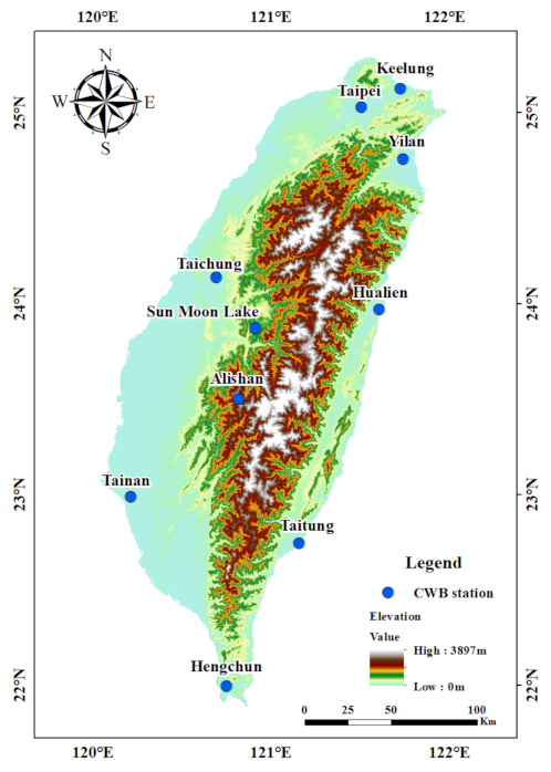
2. Study Region and Data

The region of interest in this study is the main island of Taiwan, as shown in Figure 1. Taiwan’s climate is generally warm and humid, and rainfall in Taiwan can take place nearly all year round. During late spring and early summer, persistent stationary fronts can induce significant rainfall, which is known as the Mei-Yu or plum-rain season. In summer and autumn, typhoons and accompanied southwesterlies can trigger torrential rainfall events. Even in winter, the winter monsoon can also provide some mild to substantial rainfall in the northeastern part of Taiwan. Even though seasonal rainfall in Taiwan seems to be quite abundant (annual total ≈2500 mm on average), it shows pronounced spatial variability. Due to various conditions (e.g., wind directions and topography), the seasonal pattern of rainfall resembles a uniform distribution in northern and eastern Taiwan, but exhibits a unimodal summer peak in central and southern Taiwan. Because of such high spatiotemporal variability, in company with the influence of climate oscillations [19], multiple historical drought events have still been witnessed. In fact, people in Taiwan just experienced an unprecedented drought event in nearly 60 years from late 2020 to middle 2021.

To perform drought analysis in Taiwan, we use both gauge and gridded rainfall data. Gauge rainfall data are obtained from Taiwan’s Central Weather Bureau (CWB), and we select 10 stations with extended rainfall records located evenly in different regions of the island (Figure 1). Gridded rainfall data are obtained from the Taiwan Climate Change Projection and Adaptation Information Platform (TCCIP). The development of the TCCIP dataset involves the use of rainfall gauges from as many sources as possible, including the CWB, Civil Aeronautics Administration, Water Resources Agency, Environmental Protection Administration, and Taiwan Power Company. TCCIP applies sophisticated interpolation techniques to the production of gridded rainfall data for the whole Taiwan’s territory at a 5-km spatial resolution and daily time step, and the currently available data range from 1960 to 2019. As still the best available gridded data, the TCCIP dataset has been applied to a number of studies (e.g., [3,16,20]). To suit our need for calculating the SPI series, we have aggregated both the gauge and TCCIP data at the daily time scale to monthly.

3. Methodology

This study aims at discussing whether statistically significant trends are truly meaningful through cross-referencing selected trend detection methods based on linear and smoothing techniques. Our discussion is encapsulated in (but not limited to) drought analysis in Taiwan by means of calculating and analyzing the standardized precipitation index (SPI) over 3-, 6-, 9-, and 12-month periods (hereafter SPI3, SPI6, SPI9, and SPI12) at each of the 10 gauges, as well as TCCIP’s precipitation data grids from 1960 to 2019. Simple LR is adopted as the linear technique; the slope coefficient in LR, estimated by the least squares (LS) method, can be used to indicate trends in climate time series. Regarding the smoothing technique, we use a novel spline function referred to as regularized minimal-energy tensor-product splines (RMTS) recently developed by [21] to derive two other trend detection methods: (1) locally weighted least square regression and (2) first derivatives of the fitted curve. In the following subsections, we will briefly explain the calculation procedure of the SPI, followed by the formulation of RMTS and the concept of three trend detection methods.

3.1. Standardized Precipitation Index (SPI)

The SPI, proposed by [22], is one of the indices used to evaluate the intensity of meteorological drought at varied time scales. The SPI is actually a Z score index derived from precipitation data accumulated over a specific q-month period, expressed as

$$SP{I}_q=\frac{P_q-\overline{P_q}}{S_{P_q}},$$

(1)

where $P_q$ is q-month aggregated precipitation, $\overline{P_q}$ the long-term mean of $P_q$, and $S_{P_q}$ the standard deviation of $P_q$. Since precipitation data usually do not follow a normal distribution, many studies first fitted $P_q$ to the gamma distribution, and then conducted a transformation of the cumulative probability to find the Z score [23]. When the dimensionless SPI value is negative, it indicates the climate is in a dry condition; the SPI values −1.0, −1.5, and −2 are typically used to define the categorical thresholds of drought from moderate, severe, and extreme drought, respectively.

In this study, four time scales, namely 3-, 6-, 9-, and 12-month periods, are used to calculate the SPI at each TCCIP’s precipitation data grid. We will then be able to apply trend detection to the SPI time series for the exploration of spatiotemporal variability of drought conditions across Taiwan over the previous 60 years.

3.2. Smoothing Technique: Regularized Minimal-Energy Tensor-Product Spline (RMTS)

As one of the “surrogate modeling” techniques, RMTS was developed by [21] for fitting relatively low-dimensional problems (up to four dimensions). RMTS formulates spline interpolation with a large number of spline coefficients that potentially outnumbers the training points as a regularized minimal-energy equation, and the nonlinearity of such formulation can also enhance fitting accuracy. The purpose of surrogate modeling is to replace a computationally expansive model in engineering applications with such a data-driven or curve-fitting approach as RMTS. If trained with large datasets, RMTS is known to show no convergence difficulties and can achieve fast prediction.

The prediction equation for RMTS can be expressed as

$$y=F\left(x\right)\omega ,$$

(2)

where $x\in {\mathbb{R}}^{n_x}$ is the input vector, $y\in \mathbb{R}$ the prediction output, $\omega \in {\mathbb{R}}^{n_{\omega }}$ the vector of spline coefficients, and $F\left(x\right)\in {\mathbb{R}}^{n_{\omega }}$ the mapping function of the spline coefficients to the prediction output by means of the basis function $b_{k,i}$, which can be further expressed as

$$F\left(x\right)=\sum _{i_1,\dots ,i_{n_x}}{b}_{1,i_1}\left(x_1\right)\dots b_{n_x,i_{n_x}}\left(x_{n_x}\right).$$

(3)

The estimate of spline coefficients $\omega$ is obtained from an unconstrained energy minimization problem in which the objective function is composed of three terms, as shown in Equation (4),

$$\underset{\omega }{min}\frac{1}{2}{\omega }^{T}H\omega +\frac{1}{2}\beta {\omega }^T\omega +\frac{1}{2}\frac{1}{\alpha }\sum _i^{n_t}{[F\left(x_t^{\left(i\right)}\right)\omega -y_t^{\left(i\right)}]}^2,$$

(4)

where $x_t^i\in {\mathbb{R}}^{n_x}$ is the ith training vector, $y_t^{\left(i\right)}\in \mathbb{R}$ the ith training output, $H\in {\mathbb{R}}^{n_{\omega }\times n_{\omega }}$ the discretized matrix for the continuous energy functional associated with the second-order derivatives of the spline curve, and $\alpha$ and $\beta$ are regularization coefficients. These three terms from left to right represent the energy term, regularization, and error in fitting the training points, respectively. For problems with a small number of training points, it is necessary to minimize the energy term. In contrast, for problems with a large number of training points (>1000), the energy term is optional in Equation (4); in fact, when the true function exhibits large variations in curvature, energy minimization might increase the training error. To resolve this issue, ref. [21] advised the use of a higher order for the third term in Equation (4), yet multiple iterations of Newton’s method are required. The above descriptions provide a high-level overview of RMTS; more technical details and application results of the aerodynamic and propulsion models can be found in [21].

In this study, the implementation of RMTS is through the use of the Surrogate Modeling Toolbox (SMT, ref. [24]), which is an open-source Python package consisting of many surrogate modeling techniques. In SMT, RMTS comes with two options of splines: B-splines (RMTB) and cubic Hermite splines (RMTC). Differences in the specifications of RMTB vs. RMTC (e.g., a uniform knot vector in each dimension for RMTB and continuous values and derivatives for adjacent tensor-product cubic elements for RMTC) result in the trade-off between efficiency and accuracy. If training time (accuracy) is the most important, RMTB (RMTC) is suggested. We use RMTB for the ensuing trend analysis. When using RMTB in SMT, we can specify pertinent parameter values from a list of options to pursue the best fitting performance; however, in our case, to ensure absolute consistency in fitting the SPI series at each TCCIP’s grid, we stick to those default values for RMTB, except for the number of B-spline control points in each dimension adjusted from 15 (default) to 30, in accordance with the suggestion by [18].

3.3. Trend Detection Based On Linear and Smoothing Techniques

3.3.1. Linear Regression

LS-based simple linear regression is one of the classical and widely used methods for detecting linear trends in climate time series. In this method, the observed climate variable and time sequences are taken as the response Y and independent variables X, respectively (Equation (5)). The slope and intercept coefficients (${\beta }_0$ and ${\beta }_1$) in the best fitting line can be solved by using LS, which is to find the coefficient values that minimize the square difference between the observed and predicted values of Y.

$$Y={\beta }_0+{\beta }_{1}X.$$

(5)

Trend derived from LR is determined by the slope coefficient, and its LS estimate can be expressed as

$${\beta }_1=\frac{\sum (x-\overline{x})\times (y-\overline{y})}{\sum {(x-\overline{x})}^2}.$$

(6)

The sign of the slope coefficient thus indicates trend direction (i.e., positive upward and negative downward), and the significance of upward/downward trend is usually assessed by checking the p-value of the slope coefficient. A common choice of p-value is <0.05 for a significant trend.

3.3.2. Locally Weighted Least Squares Regression

Apart from classical LS, a moving least squares regression smoother was developed by [25] for analyzing data on lead intoxication. This technique is also referred to as locally estimated scatterplot smoothing (LOESS) or locally weighted scatterplot smoothing (LOWESS), as it was initially developed for scatterplot smoothing. Ref. [26] later applied LOESS for analyzing trend for breeding bird survey data. The LOESS-based trend detection method seeks a polynomial/curve fitted to observed data, and uses such polynomial for depicting the characteristics of variations in data series. The best fitting curve is found using locally weighted LS; the basic idea is to assign a higher (lower) weight to points closer to (farther from) the fitted curve in a local area. After finding the best fitting curve, we can follow [18,26] to analyze trend for time series data. We first compute the estimate of the “route $\Delta$”, defined as the subtraction of the average of the first three fitted values from the average of the last three fitted values. The sign of $\Delta$ indicates trend direction (i.e., positive upward and negative downward). The significance of trend, according to [18,26], can be determined by the Z-test, which transforms $\Delta$ to the Z score:

$$z=\frac{\Delta }{SE(\Delta )}.$$

(7)

$SE(\Delta )$, as the standard deviation of the route estimate, is found from the bootstrap procedure: estimating m replications of $\Delta$ by resampling the observed paired data (i.e., observed climate variable and time sequences) with replacement, and then calculating the standard deviation of the m replications of $\Delta$ to obtain $SE(\Delta )$. A significance level 0.05 corresponding to $\left|z\right|>1.96$ can then be used to reject the null hypothesis of no trend ($H_0:\Delta =0$).

It can be noticed that the LOESS-based trend detection method only takes the resulting fitted curve into account, irrespective of the specifications of locally weighted least squares and the polynomial. Thus, in this study, we use the aforementioned RMTS formulation (RMTB in specific) as a representation of LOESS to find the best fitting curve, and then follow the descriptions above to analyze LOESS-based trend.

3.3.3. Test for Trend Using First Derivatives

Since the underlying assumption of simple linear regression is the constant rate of change in data, the slope coefficient is adopted as the only measure of trend. Nevertheless, in a scenario when this assumption is violated, examining the first derivatives of the fitted curve can disclose valuable information about trend. To exemplify the concept of first-derivative-based trend, we use the formulation of LS regression as guided by [18]. Consider the LS estimate of the fitted line as

$$\widehat{f}\left(x\right)=\mathbf{X}\widehat{\beta }.$$

(8)

It is straightforward to find the first derivative of $f\left(x\right)$ with respect to x,

$${\widehat{f}}^{\prime }\left(x\right)={\mathbf{X}}^{\prime }\widehat{\beta }=\left[\begin{array}{cc}0& 1\\ ⋮& ⋮\\ 0& 1\end{array}\right]\widehat{\beta }.$$

(9)

To obtain the sum of the first derivatives with respect to x, we let ${\mathbf{j}}^T=[11\dots 1]$, so

$$\sum _{t=1}^n{\widehat{f}}^{\prime }\left(x_i\right)={\mathbf{j}}^T{\mathbf{X}}^{\prime }\widehat{\beta }=\left[0n\right]\widehat{\beta },$$

(10)

from which we can note that $n\widehat{{\beta }_1}$ is actually the sum of the slope in LR. The variance of Equation (10) can be derived as

$$var\left({\mathbf{j}}^T{\mathbf{X}}^{\prime }\widehat{\beta }\right)={\sigma }_{ϵ}^2{\mathbf{j}}^T{\mathbf{X}}^{\prime }{\left({\mathbf{X}}^T\mathbf{X}\right)}^{-1}{\left({\mathbf{j}}^T{\mathbf{X}}^{\prime }\right)}^T,$$

(11)

where ${\sigma }_{ϵ}^2$ is the variance of the random error term $ϵ$. If we let ${\left({\mathbf{X}}^T\mathbf{X}\right)}^{-1}=\left[\begin{array}{cc}{c}_{00}& c_{01}\\ c_{10}& c_{11}\end{array}\right]$, we can further simplify the variance to

$$var\left({\mathbf{j}}^T{\mathbf{X}}^{\prime }\widehat{\beta }\right)={\sigma }_{ϵ}^2{n}^2{c}_{11}.$$

(12)

At the end, we are able to write the t-test statistic as

$$t=\frac{n{\widehat{\beta }}_1}{\sqrt{n^2{\widehat{\sigma }}_{ϵ}^2{c}_{11}}}=\frac{{\widehat{\beta }}_1}{{\widehat{\sigma }}_{ϵ}\sqrt{c_{11}}}=\frac{{\widehat{\beta }}_1}{SE\left({\widehat{\beta }}_1\right)}.$$

(13)

It should be noticed again that the above derivations are just an example using LS regression, and first-derivative-based trend is not limited to the LR line. In fact, if we can calculate the sum of the first derivatives $S\left(x\right)={\sum }_{i=1}^n{\widehat{f}}^{\prime }\left(x_i\right)$ of any fitted curve and the associated standard deviation, we can follow the t-test to examine the significance of trend. For other fitted curves than the LR line, it might be more difficult to derive the explicit standard deviation of $S\left(x\right)$. Ref. [18] suggested a randomization test bearing much similarity with the bootstrap procedure used in LOESS to derive the standard deviation and to conduct the t-test: estimating m replications of $S\left(x\right)$ by resampling the observed paired data with replacement, and then calculating the standard deviation of the m replications of $S\left(x\right)$ to obtain $SE\left(S\right(x\left)\right)$. Given very high degrees of freedom (>700 in our case), a significance level 0.05 corresponding to $\left|t\right|>1.96$ can then be used to reject the null hypothesis of no trend ($H_0:S\left(x\right)=0$).

As long as the first derivatives of the fitted curve can be computed, the above procedure is irrespective to the derivation of the fitted curve. Similar to the LOESS-based trend detection method, we use RMTB as the best fitting curve, from which the first derivative at each time step is available for the analysis of first-derivative-based trend.

4. Results and Discussion

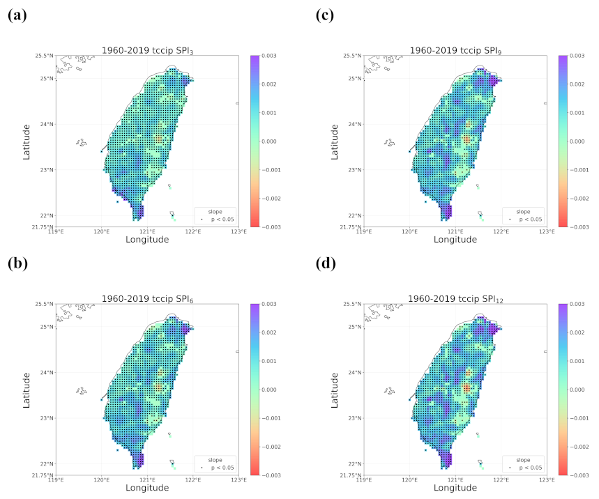
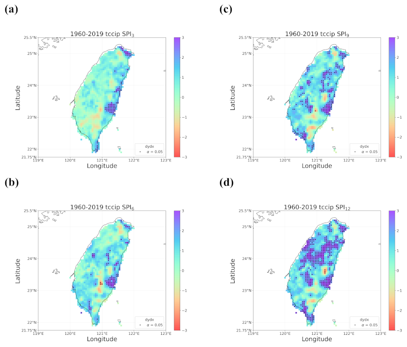
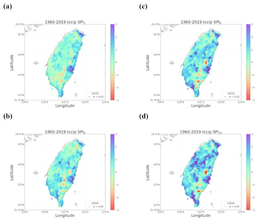
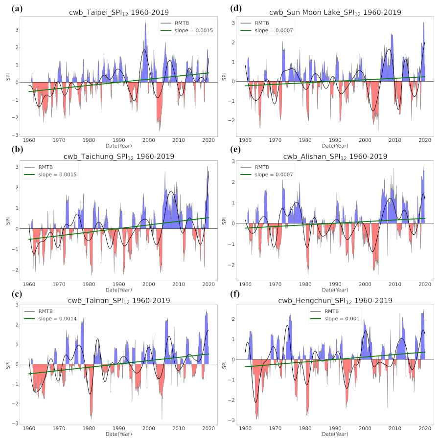
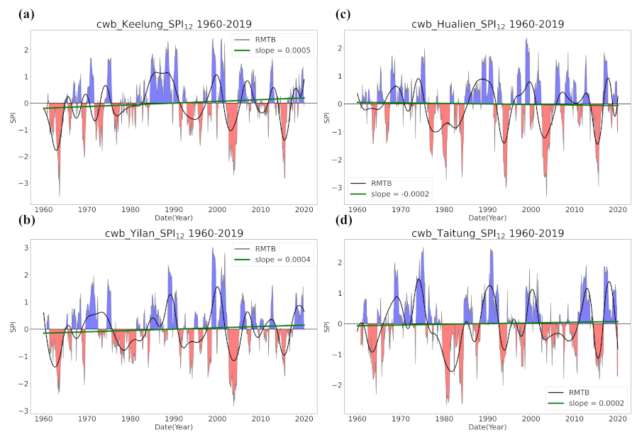
4.1. Overall Trend in Taiwan’s Drought from 1960 to 2019

After applying the three trend detection methods to the calculated SPI series at each TCCIP grid, we can show the spatial patterns of trend in drought conditions as in Figure 2, Figure 3 and Figure 4. The three trend detection methods (i.e., both linear and smoothing techniques) unanimously identify an overall upward trend in the SPI series across all four time scales in Taiwan, as a general bluish pattern can be observed. The upward trend in the SPI indicates a wetter climate condition (i.e., less and milder drought events) in the recent years compared with the earlier periods. Regarding the results of LR, we can note that significant ($p<0.05$) trends have been identified over a great portion of Taiwan’s territory (Figure 2). Such peculiar results might not reflect the true significance of the trends, but are likely to be a consequence of incorporating a large number of data in determining a less strict threshold of significance [27]. We will revisit this issue of truly significant or meaningful trend in Section 4.3.

The results based on the smoothing techniques appear to be less peculiar in terms of the portion of grids with significant trends. We can also note a progression of significant grids increasing from the SPI at a shorter time scale to a longer time scale (Figure 3 and Figure 4). The significant upward trend is observed only in the northeastern and eastern regions for SPI3, but widely distributed over the western, central, and southern regions for SPI12. There are only a few spots in sparsely populated areas showing a significant downward trend in the SPI, implying again that the condition of drought has become less severe in most areas. By comparing the first-derivative-based trend with the LOESS-based trend, we can find high pattern similarity between pairs of the SPI trend at the same time scale. However, the detected trend based on the smoothing techniques shows noticeable difference from that based on LR, especially if considering the number and location of significant grids. We will again provide more information regarding pattern similarity in Section 4.3, which could be a useful indicator for judging the comparative credibility of detected trends.

To confirm whether the overall upward trend is valid, we use the gauge data at the 10 stations to perform the same analysis. We plot the time series of SPI12 along with the best fitting line and RMTB curve for each of the stations in Figure 5 and Figure 6; the former figure shows the stations located over the western and mountainous regions, whereas the latter shows the stations over the eastern side of Taiwan. All other plots for the SPI at varied time scales are skipped because of similar results. It is clear that all the linear trend lines show a positive slope value except for station Hualien (Figure 6c), and nearly all these upward trends are statistically significant. However, it should be noticed that those SPI12 data points are scattered far away from the linear trend lines, but much closer to the RMTB curves. This might indirectly cause the problem of non-Gaussian and dependent random errors, violating the basic assumption of LR. We will keep this for further discussion later. Another point we would like to make is the regional and temporal characteristics of drought over the past 60 years. The most prominent, nationwide drought event (except the most southern–southeastern region) was the 2002 drought. After this big event, the western part of Taiwan (Figure 5) seemed to receive more precipitation than before, determining the upward trend in connection with the consecutive drought events prior to the 1990s. In contrast, over the eastern part of Taiwan (Figure 6), above-normal precipitation did not take place after 2002, and some earlier big events (e.g., the 1980 drought) seemed to be less severe. These differences in spatiotemporal characteristics motivate us to perform further examination of trend in different sub-periods next.

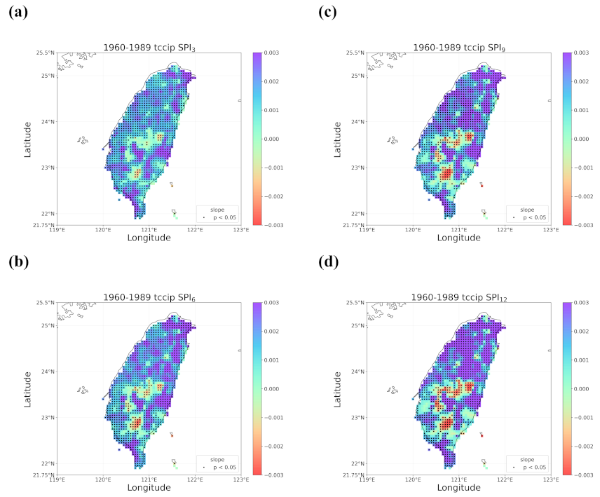
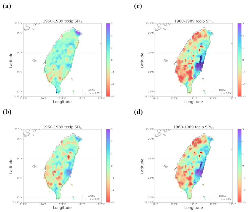
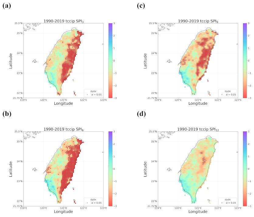
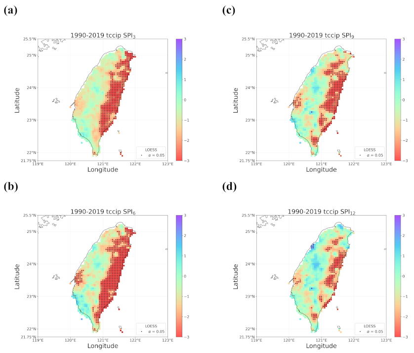
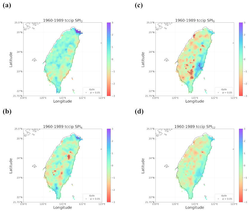
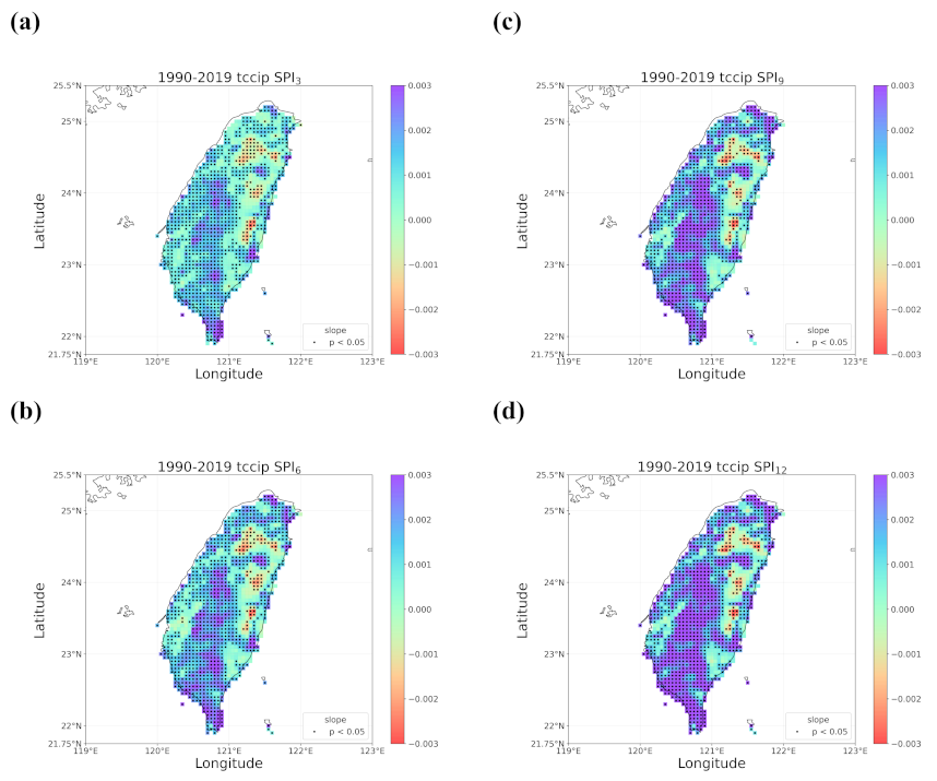
4.2. Trends in the Earlier and Later 30 Years

We follow the same procedure to perform trend detection, but instead of the entire SPI series, now we focus on the earlier 30 years (1960–1989) and the later 30 years (1990–2019) separately. Figure 7, Figure 8 and Figure 9, respectively, display the results of linear trends, first-derivative-based trends, and LOESS-based trends for the earlier 30 years. Unlike the overall upward trend identified for the entire period, the three trend detection methods all point out a downward trend over several regions in Taiwan; this is most significant (and consistent) over the southcentral mountains to the southwestern regions for the SPI at longer time scales (SPI9 and SPI12). The results of LR still exhibit many grids with significant trends (Figure 7), due to the aforementioned effect of a large number of data (still >350 data points for half of the series). While only a few grids with significant trends across four time scales are found using first derivatives (Figure 8), the significant upward trend over the northeastern coast of Taiwan is consistent with that found by the other two methods. In addition to the southwestern region, the LOESS-based method also identifies significant downward and upward trends over the northwestern and some eastern grids, respectively (Figure 9). In fact, our findings of the wetting trend over the northeast and the drying trend over the southwest by the 1990s are supported by the findings in [12], as described in Section 1.

Following the same procedure, we produce and show the results of linear trends, first-derivative-based trends, and LOESS-based trends for the later 30 years in Figure 10, Figure 11 and Figure 12, respectively. In contrast to the results of the entire period or the earlier 30 years, more obvious downward trends are identified over many regions in the later 30 years especially by two smoothing techniques (Figure 11 and Figure 12). Furthermore, such downward trends that span a large portion of eastern Taiwan across all the time scales of the SPI are clear evidence for all the three methods. We believe the more consistent results lead to a trustworthy sign of more and more severe drought events or drier conditions over eastern Taiwan if looking at the second half of the time series (e.g., Figure 6). The pronounced drier conditions in the recent period can easily be concealed with different interval selection (e.g., comparing Figure 10, Figure 11 and Figure 12 with Figure 2, Figure 3 and Figure 4). Apart from the drying trends, from the central mountains to the southwestern coast, there seems to be an upward trend in the SPI across the time scales, yet the significance can only be denoted by LR. It should be noticed that, while some clear migrations of drying or wetting patterns can be identified using different time intervals, there is no (and should not be any) universal rule with regard to the most adequate interval selection. Researchers should be aware of the influence of interval selection and be responsible for explaining the cause of varied trends.

It is intuitive that better consistency of the trend patterns should be maintained by the two smoothing methods since the same fitted RMTB curve is used for a designated grid. Nonetheless, more obvious discrepancies between the first-derivatives-based trend pattern and the LOESS-based trend pattern can be noticed in either of the sub-periods (e.g., Figure 8d vs. Figure 9d or Figure 11d vs.Figure 12d), as opposed to the entire period (e.g., Figure 3 vs. Figure 4). If scrutinizing the results further, we find that the discrepancies are actually a result of the difference in the amount of significant grids. LOESS appears to be “more sensitive” to the number of data points, thereby identifying more grids with significant trends when the entire series is cut in half. If eliminating the influence of the amount of significant grids (i.e., ignoring the dots in Figure 8, Figure 9, Figure 11, and Figure 12), we can still find that the two smoothing methods can maintain good consistency of the trend patterns.

Another notable difference between the trend detection method using first derivatives and LOESS that should be addressed is the number of fitted data points used for deriving the trend statistics: the former has to make use of the first derivatives at all the points by design, while the latter takes only the first three and last three fitted values into account (see Section 3.3.2 and Section 3.3.3). In fact, such a specific way to estimate the route of a fitted RMTB curve introduces another degree of freedom to LOESS. For instance, if we use fewer or more fitted values to estimate the route, the resulting Z score (Equation (7)) will be different. To verify this point, we have taken the RMTB curve for SPI12 at Taitung station (see Figure 6d) as an example, (Figure S1) and recalculated the Z scores as a function of the number of fitted values (Figure S1). We have found that because the Z score can vary drastically, LOESS is indeed more sensitive and may have a higher chance to identify more grids with significant trends. In this regard, the lower sensitivity of the trend detection method using first derivatives becomes one of its advantages over LOESS.

4.3. Discussion of Meaningful Trends

The above two sub-sections have disclosed how Taiwan’s drought conditions varied over the past 60 years, and the results of trend detection have shown drastic differences using the different trend detection methods and time intervals. In this sub-section, we wish to address those outstanding questions previously raised, and eventually offer a rule of thumb regarding the judgment of truly meaningful trends. Firstly, we would like to deal with the excessive amount of significant grids resulting from LR trend detection. According to [27], it is natural to have a deflated significance level with many data points, but the real concern should be the overly scattered points away from the trend lines, causing the probable violation of normality and independent assumptions for the random error term [17]. To verify whether the normality assumption has been held in our case, we apply the Shapiro–Wilk test [28] to the residuals of the previously fitted LR models for the SPI at all the grids from 1960 to 2019. If it is required that not only the significance of slope but also normal random errors should be satisfied, we will see a sharp reduction in the number of points labeled on the plots (Figure S2). The normality assumption is clearly violated. If taking one step further to examine whether the LR models generate a reasonable fit to data series using $R^2=0.65$ as the threshold [27], we will also obtain similar plots with sparsely distributed points (Figure S3). According to the above findings, LR should better be excluded from the use of trend detection in hydroclimate time series due to its presumably inherent nonlinearity.

The second outstanding question is whether we can quantify pattern similarity between pairs of detected trends based on different methods, as an indicator for revealing trends with higher credibility. Calculating pattern correlation between two maps of trend statistics (e.g., Figure 2 vs. Figure 3) is an intuitive means to quantify pattern similarity; further, to emphasize trends with significance identified by different methods, we convert significantly upward (downward) trend statistics to 1 (−1) and all remaining insignificant trend statistics to zeros prior to calculating pattern correlation. For instance, if the Z score is the trend statistic, Z values outside the bounds $\pm 1.96$ will be converted to $\pm 1$, and Z values within $\pm 1.96$ will be converted to zeros. We thus follow this procedure to calculate and show all the pattern correlations between pairs of the SPI trend previously obtained for the entire period (1960–2019), the earlier 30 years (1960–1989), and the later 30 years (1990–2019) in

Table 1. Pattern correlations between detected trend in the SPI using one of the three methods and that using another method over three different time periods. The first, second, and third values in each parenthesis indicate correlations derived from the paired methods: linear regression (LR) vs. first derivative; LR vs. locally estimated scatterplot smoothing (LOESS), and first derivative vs. LOESS, respectively. Correlation values greater than 0.35 are in bold.

Time Period	SPI3	SPI6	SPI9	SPI12
1960–2019	(0.03, 0.02, 0.67)	(0.04, 0.05, 0.74)	(0.09, 0.10, 0.66)	(0.19, 0.22, 0.68)
1960–1989	(0.04, 0.06, 0.79)	(0.03, 0.22, 0.44)	(0.26, 0.23, 0.37)	(0.01, 0.19, 0.08)
1990–2019	(0.32, 0.36, 0.91)	(0.40, 0.38, 0.86)	(0.49, 0.52, 0.71)	(0.28, 0.40, 0.13)

. We can note that the LR results usually do not correlate with the first derivatives or LOESS results well, especially for the SPI at the shorter time scales over the entire period or the earlier 30 years. In contrast, the first derivatives and LOESS results, as both rooted in RMTB, exhibit high pattern correlations on many occasions. If we rule out results pertaining to LR, as per the above suggestion, the correlation between the first derivatives and LOESS results seems to be a useful metric to determine how credible the detected trend is. For instance, the most credible trend would be the recent drying trend at the shorter time scales over eastern Taiwan in 1990–2019 since we observe the highest pattern correlations as 0.91 and 0.86 for SPI3 and SPI6. In fact, LR also shows some moderate correlations with the other two methods in this particular occasion, suggesting such drying trend should be trustworthy with much confidence. On the other hand, if all the correlations in one parenthesis are low in Table 1 (e.g., for SPI12 in 1960–1989), we should realize that significant trends identified by any methods are subject to high uncertainty; the method-specific significance might be nothing but a statistical fluke.

5. Conclusions and Recommendations

Various methods for trend analysis have been invented and used in hydroclimate science for better understanding how variables of interest change over time. However, interpreting the results of trend analysis may not be as trivial as one can imagine. The significance of detected trends can be contingent upon not only the target variable itself, but also several key factors, including method-specific assumptions and time interval selection. In this study, we applied linear regression and two smoothing techniques to the detection of trends in the long-term SPI series over the main island of Taiwan in order to disclose spatiotemporal variations in drought conditions. We adopted RMTB, one type of RMTS, as the basis of the smoothing techniques for the derivation of trend detection using first derivatives and LOESS. According to our analysis, we would like to make three concluding remarks:

• Trend detection using LR showed great differences from that using the smoothing techniques, and LR seemed to be less robust as it falsely identified too many grids with significant trends and non-Gaussian residuals. LR trend lines were not found meaningful in many occasions of our case examining the SPI series in Taiwan since the data did not present much linearity.
• When all the methods reached a consensus in the patterns of detected trends with significance, intuitively we could have more confidence in such detected trends. By calculating pattern correlations as the quantification metric of pattern similarity between detected trends, we found that the recent drying trend at the shorter time scales over eastern Taiwan in 1990–2019 should be the most trustworthy.
• Regardless of the methods, detected trends in the entire period (1960–2019), the earlier 30 years (1960–1989), or the later 30 years (1990–2019) were all different. While the general wetting trend was identified over a great portion of Taiwan’s territory in the past 60 years, some migrations of drying or wetting trends actually took place in different time intervals.

In sum, our analysis results showed considerable differences in intermethod comparison, the SPI at varied time scales, and time interval selection. We urge researchers in the discipline of hydroclimatology to use LR for trend detection with great caution owing to common nonlinearity and outliers in data series as well as non-normality and dependency in residuals. More robust detection methods free from the above constraints are advised, such as the generalized linear model, least median of square estimator [29], nonparametric methods, or smoothing techniques, as demonstrated in this study; however, comprehending detailed mechanisms pertaining to these methods (e.g., LOESS is sensitive to the number of points taken for the derivation of Z scores) and their own constraints would still be necessary. To verify whether the found trends are credible, cross-referencing outcomes from multiple methods (e.g., checking pattern similarity) is essential, and perhaps testing field significance [30] is also required if dealing with spatially distributed data (e.g., gridded data in our case). Another topic worth further investigation could be identifying similarity or clusters among trends in spatial data using empirical techniques (e.g., [31]). Lastly, researchers should always be responsible for explaining probably varied trends subject to time interval selection; inspecting data variability and major/extreme events in the focused time interval should be as important as revealing the overall trend.

References

1. Seager, R.; Naik, N.; Vogel, L. Does global warming cause intensified interannual hydroclimate variability? J. Clim. 2012, 25, 3355–3372. [Google Scholar] [CrossRef] [Green Version]
2. Madsen, H.; Lawrence, D.; Lang, M.; Martinkova, M.; Kjeldsen, T.R. Review of trend analysis and climate change projections of extreme precipitation and floods in Europe. J. Hydrol. 2014, 519, 3634–3650. [Google Scholar] [CrossRef] [Green Version]
3. Chen, C.J.; Chen, C.C.; Lo, M.H.; Juang, J.Y.; Chang, C.M. Central Taiwan’s hydroclimate in response to land use/cover change. Environ. Res. Lett. 2020, 15, 034015. [Google Scholar] [CrossRef]
4. Bhuyan, M.D.I.; Islam, M.M.; Bhuiyan, M.E.K. A trend analysis of temperature and rainfall to predict climate change for northwestern region of Bangladesh. Am. J. Clim. Chang. 2018, 7, 115–134. [Google Scholar] [CrossRef] [Green Version]
5. Mann, H.B. Nonparametric tests against trend. Econometrica 1945, 13, 245–259. [Google Scholar] [CrossRef]
6. Theil, H. A rank-invariant method of linear and polynomial regression analysis. Indag. Math. 1950, 12, 173. [Google Scholar]
7. Sen, P.K. Estimates of the regression coefficient based on Kendall’s tau. J. Am. Stat. Assoc. 1968, 63, 1379–1389. [Google Scholar] [CrossRef]
8. Pettitt, A.N. A non-parametric approach to the change-point problem. J. R. Stat. Soc. Ser. C Appl. Stat. 1979, 28, 126–135. [Google Scholar] [CrossRef]
9. Jiang, S.; Wang, M.; Ren, L.; Xu, C.Y.; Yuan, F.; Liu, Y.; Shen, H. A framework for quantifying the impacts of climate change and human activities on hydrological drought in a semiarid basin of Northern China. Hydrol. Process. 2019, 33, 1075–1088. [Google Scholar] [CrossRef]
10. Animashaun, I.M.; Oguntunde, P.G.; Akinwumiju, A.S.; Olubanjo, O.O. Rainfall analysis over the Niger central hydrological area, Nigeria: Variability, trend, and change point detection. Sci. Afr. 2020, 8, e00419. [Google Scholar] [CrossRef]
11. Harka, A.E.; Jilo, N.B.; Behulu, F. Spatial-temporal rainfall trend and variability assessment in the Upper Wabe Shebelle River Basin, Ethiopia: Application of innovative trend analysis method. J. Hydrol. Reg. Stud. 2021, 37, 100915. [Google Scholar] [CrossRef]
12. Chen, S.T.; Kuo, C.C.; Yu, P.S. Historical trends and variability of meteorological droughts in Taiwan/Tendances historiques et variabilité des sécheresses météorologiques à Taiwan. Hydeol. Sci. J. 2009, 54, 430–441. [Google Scholar] [CrossRef]
13. Shih, D.S.; Chen, C.J.; Li, M.H.; Jang, C.S.; Chang, C.M.; Liao, Y.Y. Statistical and numerical assessments of groundwater resource subject to excessive pumping: Case study in Southwest Taiwan. Water 2019, 11, 360. [Google Scholar] [CrossRef] [Green Version]
14. Yeh, H.F. Using integrated meteorological and hydrological indices to assess drought characteristics in southern Taiwan. Hydrol. Res. 2019, 50, 901–914. [Google Scholar] [CrossRef]
15. Lee, Y.C.; Wang, C.C.; Weng, S.P.; Chen, C.T. Future Projections of Meteorological Drought Characteristics in Taiwan. Atmos. Sci. 2019, 47, 66–91. [Google Scholar]
16. Henny, L.; Thorncroft, C.D.; Hsu, H.H.; Bosart, L.F. Extreme Rainfall in Taiwan: Seasonal Statistics and Trends. J. Clim. 2021, 34, 4711–4731. [Google Scholar] [CrossRef]
17. Mudelsee, M. Trend analysis of climate time series: A review of methods. Earth Sci. Rev. 2019, 190, 310–322. [Google Scholar] [CrossRef]
18. Gray, K.L. Comparison of Trend Detection Methods; University of Montana: Missoula, MT, USA, 2007. [Google Scholar]
19. Chen, C.J.; Lee, T.Y. Variations in the correlation between teleconnections and Taiwan’s streamflow. Hydrol. Earth Syst. Sci. 2017, 21, 3463–3481. [Google Scholar] [CrossRef] [Green Version]
20. Li, P.L.; Lin, L.F.; Chen, C.J. Hydrometeorological Assessment of Satellite and Model Precipitation Products over Taiwan. J. Hydrometeorol. Meteorol. 2021, 22, 2897–2915. [Google Scholar] [CrossRef]
21. Hwang, J.T.; Martins, J.R.R.A. A fast-prediction surrogate model for large datasets. Aerosp. Sci. Technol. 2018, 75, 74–87. [Google Scholar] [CrossRef]
22. McKee, T.B.; Doesken, N.J.; Kleist, J. The relationship of drought frequency and duration to time scales. In Proceedings of the 8th Conference on Applied Climatology, Anaheim, CA, USA, 17–22 January 1993; Volume 17, pp. 179–183. [Google Scholar]
23. Guenang, G.M.; Kamga, F.M. Computation of the Standardized Precipitation Index (SPI) and its use to assess drought occurrences in Cameroon over recent decades. J. Appl. Meteorol. Climatol. 2014, 53, 2310–2324. [Google Scholar] [CrossRef]
24. Bouhlel, M.A.; Hwang, J.T.; Bartoli, N.; Lafage, R.; Morlier, J.; Martins, J.R.R.A. A Python surrogate modeling framework with derivatives. Adv. Eng. Softw. 2019, 135, 102662. [Google Scholar] [CrossRef] [Green Version]
25. Cleveland, W.S. Robust locally weighted regression and smoothing scatterplots. J. Am. Stat. Assoc. 1979, 74, 829–836. [Google Scholar] [CrossRef]
26. James, F.C.; McCulloch, C.E.; Wiedenfeld, D.A. New approaches to the analysis of population trends in land birds. Ecology 1996, 77, 13–27. [Google Scholar] [CrossRef] [Green Version]
27. Bryhn, A.C.; Dimberg, P.H. An operational definition of a statistically meaningful trend. PLoS ONE 2011, 6, e19241. [Google Scholar] [CrossRef] [Green Version]
28. Shapiro, S.S.; Wilk, M.B. An analysis of variance test for normality (complete samples). Biometrika 1965, 52, 591–611. [Google Scholar] [CrossRef]
29. Muhlbauer, A.; Spichtinger, P.; Lohmann, U. Application and comparison of robust linear regression methods for trend estimation. J. Appl. Meteorol. Climatol. 2009, 48, 1961–1970. [Google Scholar] [CrossRef]
30. DelSole, T.; Yang, X. Field significance of regression patterns. J. Clim. 2011, 24, 5094–5107. [Google Scholar] [CrossRef]
31. Huang, N.E.; Shen, Z.; Long, S.R.; Wu, M.C.; Shih, H.H.; Zheng, Q.; Yen, N.C.; Tung, C.C.; Liu, H.H. The empirical mode decomposition and the Hilbert spectrum for nonlinear and nonstationary time series analysis. Proc. R. Soc. Lond. A 1971, 454, 903–995. [Google Scholar] [CrossRef]
Figure 1. The main island of Taiwan and the location of ten Central Weather Bureau (CWB) stations.
Atmosphere 13 00444 g001
Figure 2. Spatial patterns of trends in the SPI series from 1960 to 2019 detected using linear regression; (ad) the SPI at 3-, 6-, 9-, and 12-month periods. Grids with significant trends are dotted.
Atmosphere 13 00444 g002
Figure 3. The same as Figure 2, but for detected trends using first derivatives of regularized minimal-energy tensor-product B-splines (RMTB).
Atmosphere 13 00444 g003
Figure 4. The same as Figure 2, but for detected trends using locally estimated scatterplot smoothing (LOESS).
Atmosphere 13 00444 g004
Figure 5. SPI12 time series along with the best fitting linear trend lines and RMTB curves at six CWB stations located over the (ac) western, (d,e) mountainous, and (f) southern regions of Taiwan.
Atmosphere 13 00444 g005
Figure 6. The same as Figure 5, but for four CWB stations over the eastern side of Taiwan.
Atmosphere 13 00444 g006
Figure 7. Spatial patterns of trends in the SPI series in the earlier period (1960–1989) detected using linear regression; (ad) the SPI at 3-, 6-, 9-, and 12-month periods.
Atmosphere 13 00444 g007
Figure 8. The same as Figure 7, but for detected trends using first derivatives of RMTB.
Atmosphere 13 00444 g008
Figure 9. The same as Figure 7, but for detected trends using LOESS.
Atmosphere 13 00444 g009
Figure 10. Spatial patterns of trends in the SPI series in the later period (1990–2019) detected using linear regression; (ad) the SPI at 3-, 6-, 9-, and 12-month periods.
Atmosphere 13 00444 g010
Figure 11. The same as Figure 10, but for detected trends using first derivatives of RMTB.
Atmosphere 13 00444 g011
Figure 12. The same as Figure 10, but for detected trends using LOESS.
Atmosphere 13 00444 g012