Article

Analysis of the Factors Having an Influence on the LC Passive Harmonic Filter Work Efficiency

by
Chamberlin Stéphane Azebaze Mboving
*,
Zbigniew Hanzelka
* and
Andrzej Firlit
Department of Power Electronics and Energy Control Systems, Faculty of Electrical Engineering, Automatics, Computer Science and Biomedical Engineering, AGH University of Science and Technology, 30-059 Krakow, Poland
*
Authors to whom correspondence should be addressed.
Energies 2022, 15(5), 1894; https://doi.org/10.3390/en15051894
Submission received: 6 February 2022 / Revised: 21 February 2022 / Accepted: 27 February 2022 / Published: 4 March 2022

Abstract

:
This paper presents the electrical system factors having an influence on the work efficiency and performance of the LC passive harmonic filters (PHFs). Such filters are very often used in industries for the purpose of harmonics mitigation and reactive power compensation. Before their installation in the electrical system, many investigations should be performed in order to ensure their good design as well as work efficiency after connection. In this paper, the factors having an influence on the PHFs work efficiency and performance, such as the grid short-circuit power, primary grid voltage spectrum (voltage measured at the PCC before the filter connection), load reactive power and current characteristic harmonics, manufacturer filter parameters tolerance and filter-detuning phenomena are investigated. Most of the quoted factors are mentioned in the literature, but the novelty of this paper is that, based on the case study example of the single-tuned filter investigated in the laboratory, the influence of those factors on the filter work efficiency are demonstrated, and some solutions and recommendations are proposed. The studies are focused on the design of the single-tuned filter in the laboratory, and some simulation results are presented as well.

1. Introduction

With the increasing number of non-linear loads as well as distributed electrical energy sources with power electronic interfaces, many solutions in terms of power quality disturbances mitigation are proposed. Nowadays, active and hybrid solutions are in full growth, and their main drawbacks in comparison to the passive solutions (PHFs) are their high price and complexity in the control system [1,2,3,4]. Despite their disadvantages (e.g., harmonics amplification, detuning phenomena, electrical grid dependency of their efficiency, the choice of the damping resistance, etc.), PHFs are commonly used in practice because they are low cost, simple in structure, easy to maintain, highly efficient in terms of individual harmonic reduction, and have easy applicability in low voltage (LV), medium voltage (MV), and high voltage (HV) systems [5,6,7]. The PHFs are organized in different structures described in the literature [8]: the single-tuned filter [9,10,11,12,13,14,15,16], double-tuned filter [17,18,19,20,21,22,23,24,25,26,27,28], triple-tuned filter [29,30], series passive filter [31], hybrid passive filter [32,33], damped filters (first, second, third-order filter, and C-type filter) [34,35,36,37,38,39,40,41], filter group [42,43,44,45,46,47,48,49], etc.
In most cases, the PHFs are applied in the electrical system in order to mitigate harmonics and reactive power. The consequences of the reactive power generated in the electrical system can be the system instability, which can affect the voltage and current level, the change of the system power losses, which may increase, etc. [50,51,52]. The harmonic sources in the power system can be organized into three important groups such as presented in [53]: saturated core devices (e.g., transformers, motors, generators, etc.); arc devices (e.g., arc furnaces devices, welding devices, gas-discharge lamp, etc.), and electronic or power electronic devices. The harmonics, if not mitigated in the electrical system, can cause: the increase in voltage and current true RMS, the overloading, overheating, and even damage of electrical system elements (e.g., transformers, generators, cables, electric motors, capacitors, etc.) and other connected devices, the reduction in a device’s life span, the perturbation of the devices normal operation and increase in operating costs, the inaccurate measurements of energy and power and the decrease in power factor (PF), etc. [54,55,56,57,58].
For the PHFs to mitigate the unwanted harmonics efficiently, many electrical system factors needed to be taken into account and be well investigated. Those factors are, among others, the grid short-circuit power, which includes the grid impedance of the harmonic to be eliminated, the primary grid voltage spectrum (voltage measured at the PCC before the filter connection), the load reactive power and current characteristic harmonics, manufacturer filter parameters tolerance, and the filter-detuning phenomena, which may lead to harmonics amplification. Most of the above-quoted factors are also mentioned in the literature [59,60], but the experimental demonstrations of some of them (for instance, how the harmonics flowing from the electrical grid (because of the distorted supply voltage) disturb the filter work efficiency) are rare in the literature. This paper presents a case study in which those factors are highlighted (demonstrated) and investigated in the laboratory and by simulation, and some solutions and recommendations are proposed. The case study concerns the design of the single-tuned filter from the computation of the parameters to its connection in the laboratory setup.
In this paper, it is experimentally demonstrated that the electrical grid seen from the point of the laboratory setup connection behaves as a source of current harmonics, which flows through the filter and reduces its work efficiency in terms of harmonics mitigation and that the manufacturer tolerance of the filter parameters influences the filter effectiveness. The experiments concerning the detuning of the PHF are presented as well. All the details of the laboratory investigation before and after the filter connection are described in the paper: the investigation on the electrical system parameters before the filter and load connection; observation of the voltage and current harmonics behavior after the load connection (without filter) by changing the values of load current harmonics; laboratory measurements of the filter parameters and characteristics; connection of the filter in the laboratory setup and investigation on the factors having an influence on its work efficiency using a programmable voltage source. The investigations and results presented in this paper are based on laboratory experiments, and some simulations (MATLAB/SIMULINK [61]) are also presented to clarify the laboratory investigations. The laboratory data are measured through the PQ analyzer hardware “PQ-Box 200” [62]. Since the power system of the designed laboratory model is symmetrical, the results are focused on one phase.
The next sections of this paper are organized as follows: Section 2 presents the laboratory setup, the investigations performed before and after the filter connection, additional experiments with the programmable AC voltage source together with recommendations. Section 3 presents the conclusion, and the last section is about the Appendix A.

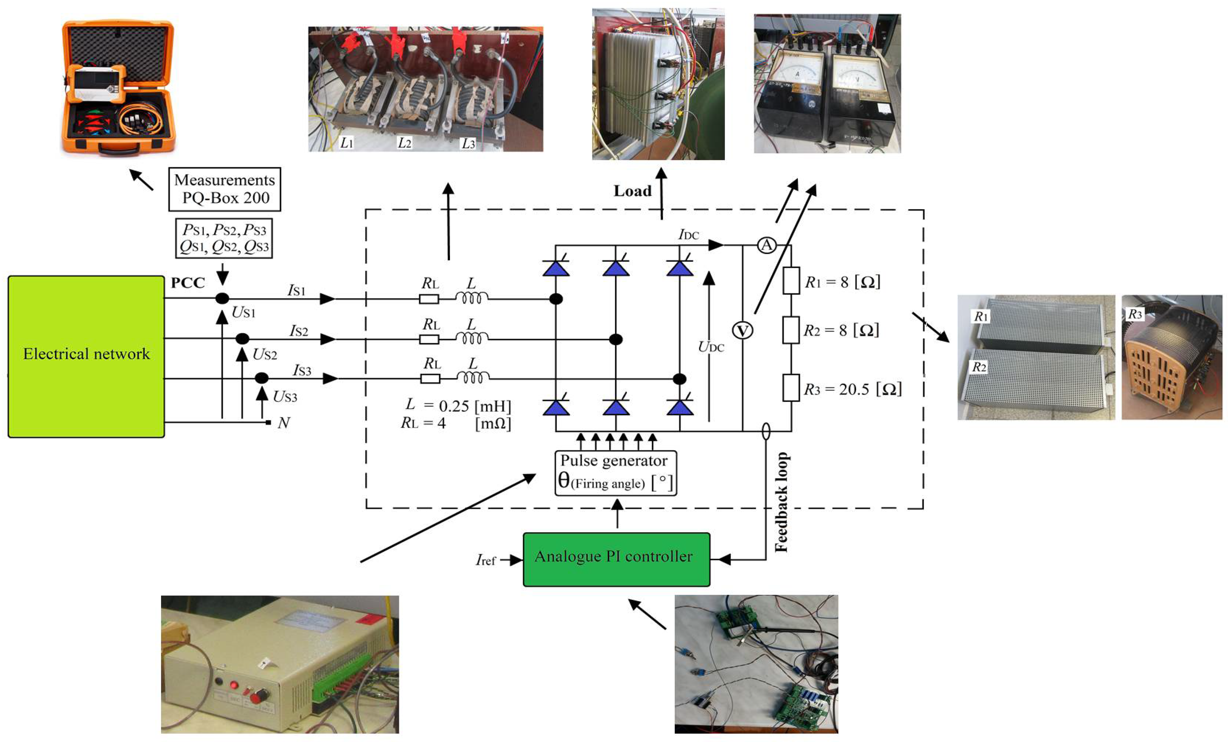
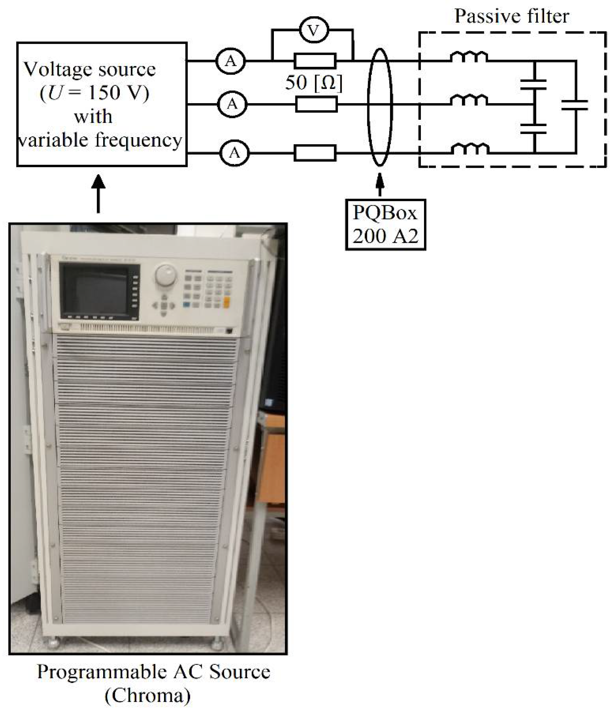
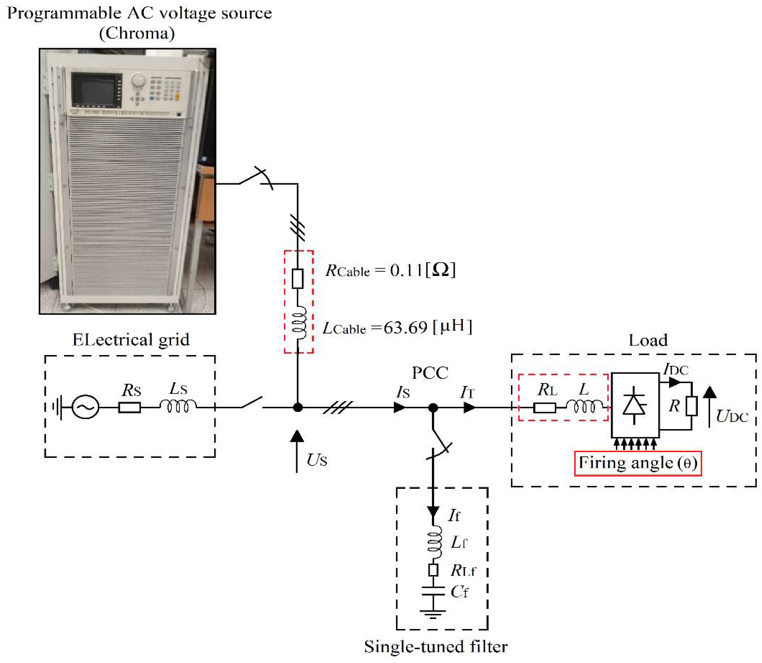
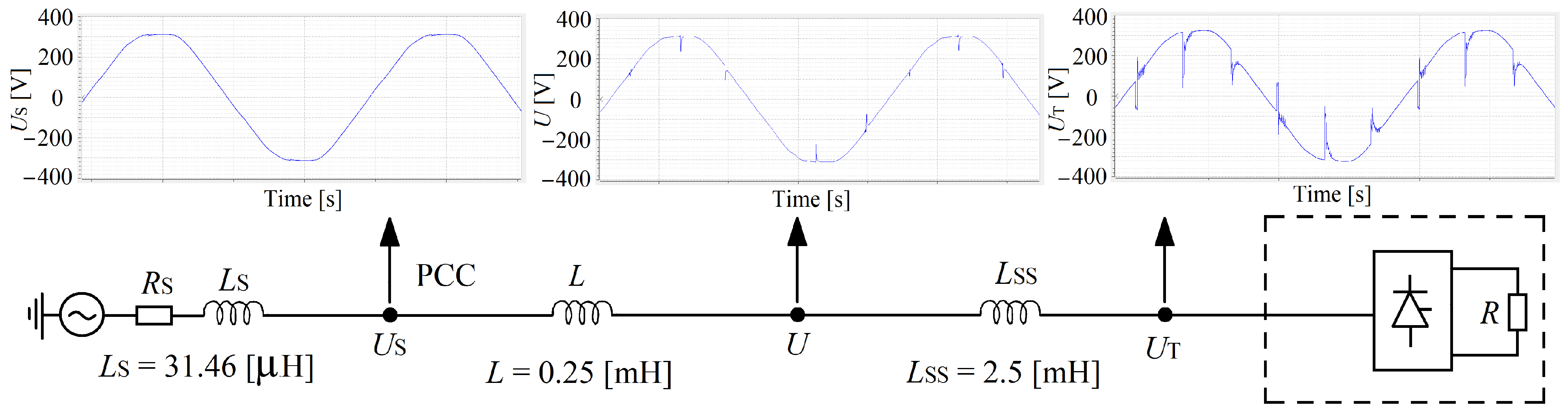
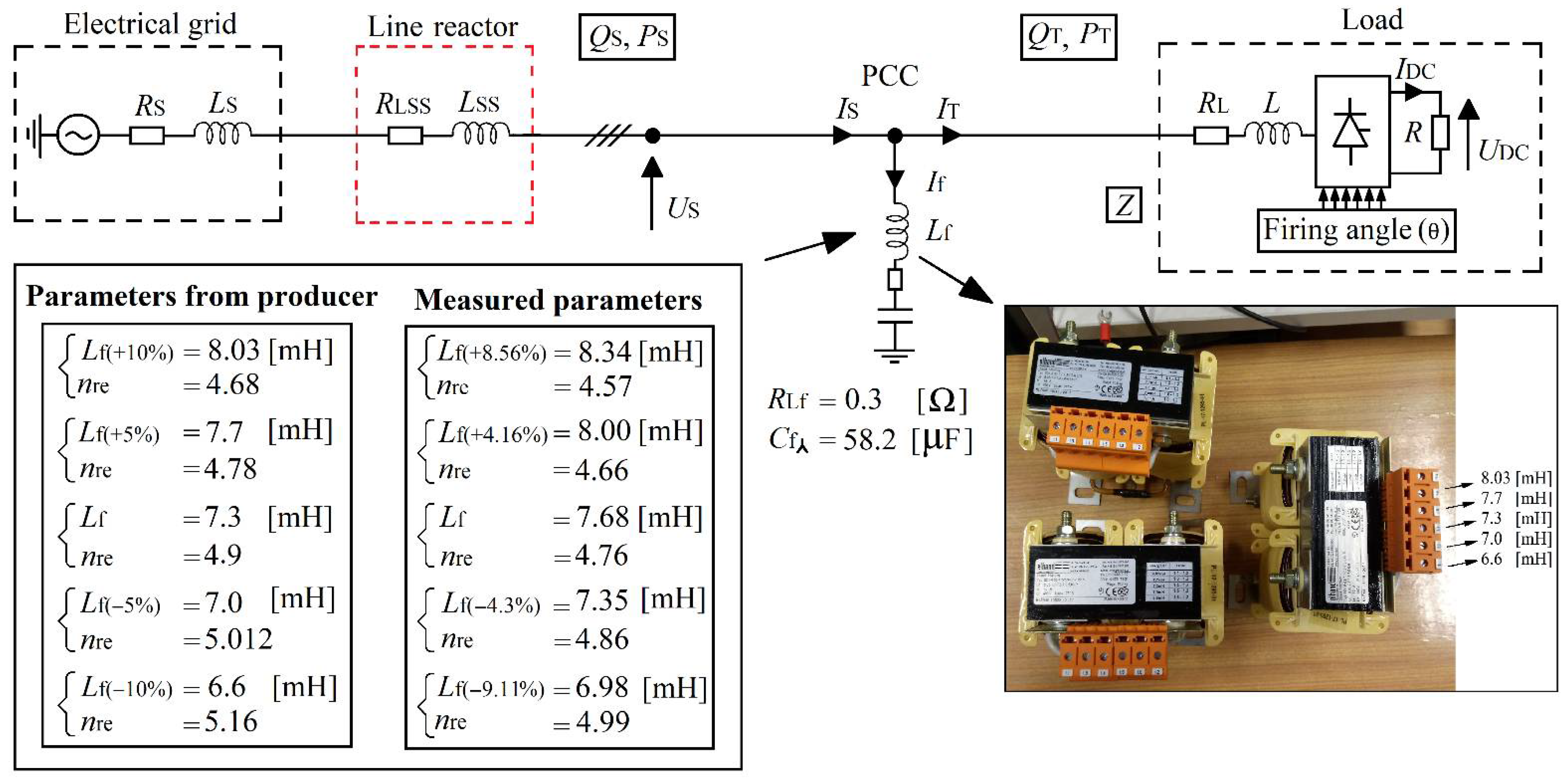
2. Laboratory Model Description

The block diagram representing the laboratory model is presented in Figure 1. It is constituted of the electrical network (grid) and the load. Before the single-tuned filter connection at the PCC, some investigations were performed at the PCC when the load was not connected and when it was connected.

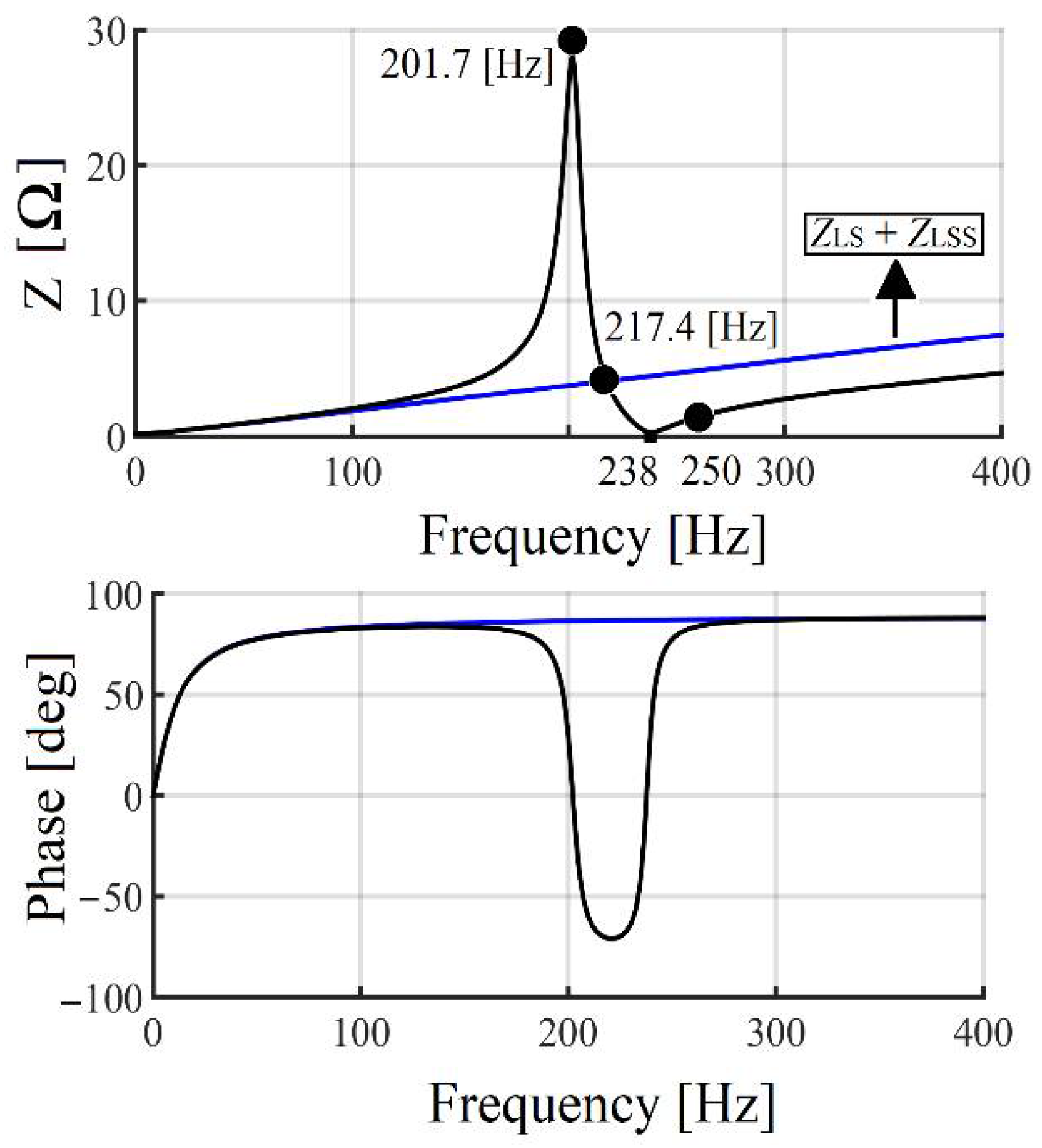
2.1. Studies of the Electrical Network before the Filter and Load Connection

The goal of performing such studies is to estimate the grid equivalent impedance of harmonic to be eliminated (e.g., ZS(n), n-harmonic order) and to obtain information about the grid supply voltage spectrum.
The electrical grid supplying the laboratory in which the experimental studies were performed is shown in the equivalent circuit in Figure 2a. It can be noticed that the parameters of the electrical network are considered from the medium to the low voltage side. The electrical network equivalent parameters for the fundamental and 5th harmonic (impedance (ZS(1), ZS(5)), short-circuit current (ISC_Sec), and power (SSC_Sec)) are presented in Figure 2b.
The electrical grid voltage supplying the laboratory setup is symmetrical (the negative sequence represents around 0.12% of the positive sequence) but a bit distorted (Figure 3a) because of other connected non-linear devices. Its spectrum in Figure 3b shows that the dominating harmonics are the 5th (around 2%), the 3rd (more than 1%), and the 7th (almost 1%). According to the IEC61000-2-4 standard [63], its THD and harmonics amplitude are acceptable (Figure 3b).

2.2. PCC Parameters Analysis after the Load Connection

The designed laboratory non-linear load is constituted of a six-pulse thyristor bridge (rectifier) with input reactor (L) at the AC side and resistance at the DC side (the total resistance of the DC side load is up to 36.5 Ω) (Figure 1).
The thyristor bridge rectifier is a dynamic device from the point of view of the variability of its firing angle. Because of that, it was important to investigate (in the laboratory) the firing angle boundary values, the load minimum and maximum active and reactive powers, as well as the change of the amplitude of the harmonics (e.g., 5th, 7th, etc.) of the PCC voltage and current by increasing or decreasing the firing angle. The formula of the load characteristic harmonics order is n = (6k ± 1), where k is a natural number.
After its connection at the PCC (Figure 1), the load was analyzed by increasing the DC voltage from 0 V to 525 V (decrease in the firing angle). The recorded data were analyzed through the MATLAB tools by means of the fast Fourier transformer (FFT) algorithm.

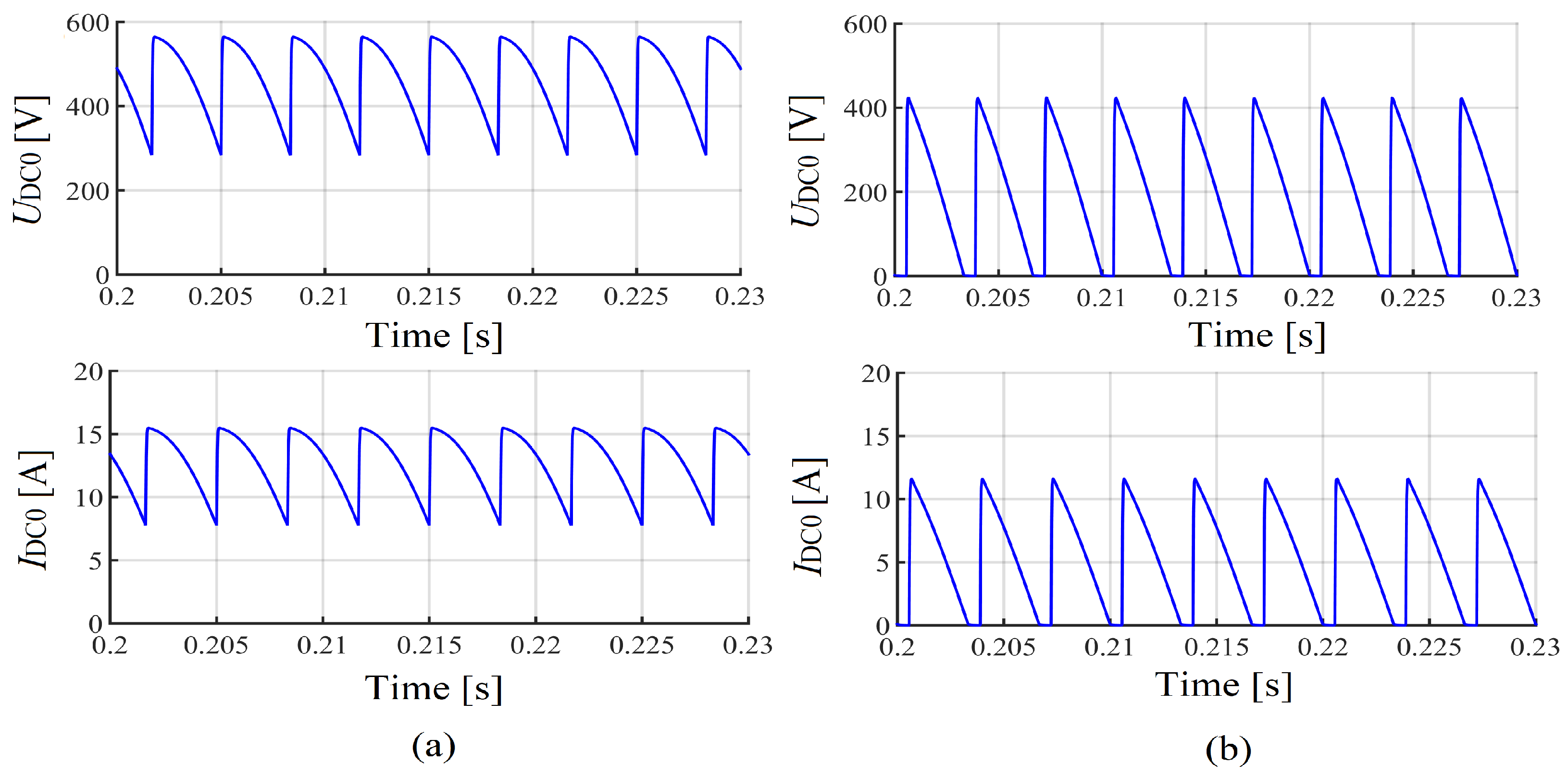
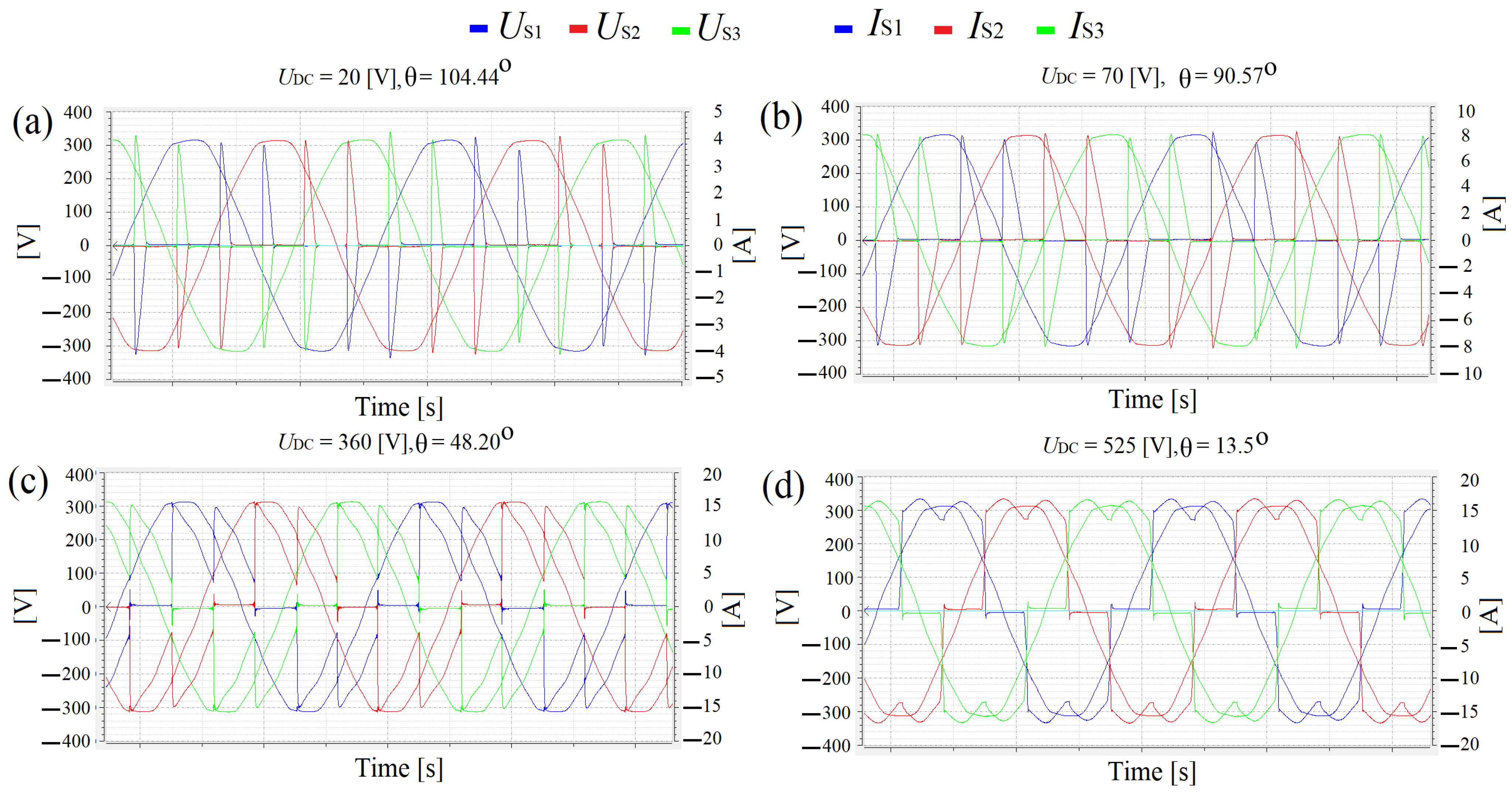
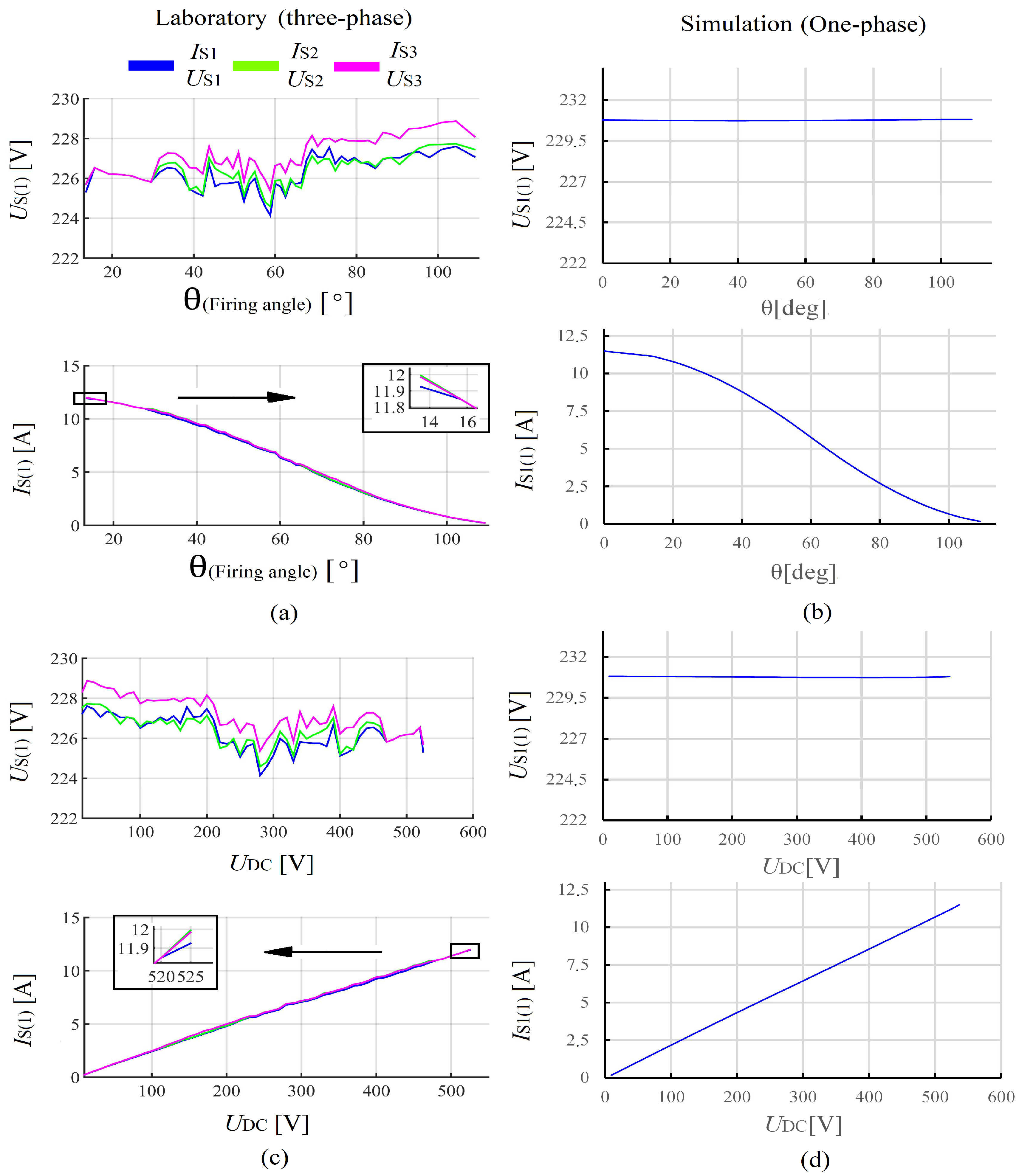
2.2.1. Investigation on the Boundary of the Rectifier Firing Angle

With the resistance connected at the rectifier DC side, the firing angle (θ) boundary can be estimated through Equations (1) (continuous DC voltage and current) and (2) (discontinuous DC voltage and current); the thyristor commutation coefficient is not considered [64]. The continuous and discontinuous mode of the DC voltage and current are more clarified by the waveforms obtained from the simulated laboratory model (see Figure 4). Figure 5 presents an example of PCC voltage and current waveforms (form the “PQ-Box 200”) when the firing angle is decreased from 104.44° to 13.5°. See the equation [65] below:
θ = acos ( U DC 1.35 U L - L )                                 for   0 θ π 3
θ = acos ( U DC 1.35 U L - L ) 1 π 3         for   π 3 θ 2 π 3
For   2 π 3 θ π ,   U DC = 0
UL-L—line-to-line AC voltage; UDC average voltage at the rectifier DC side.

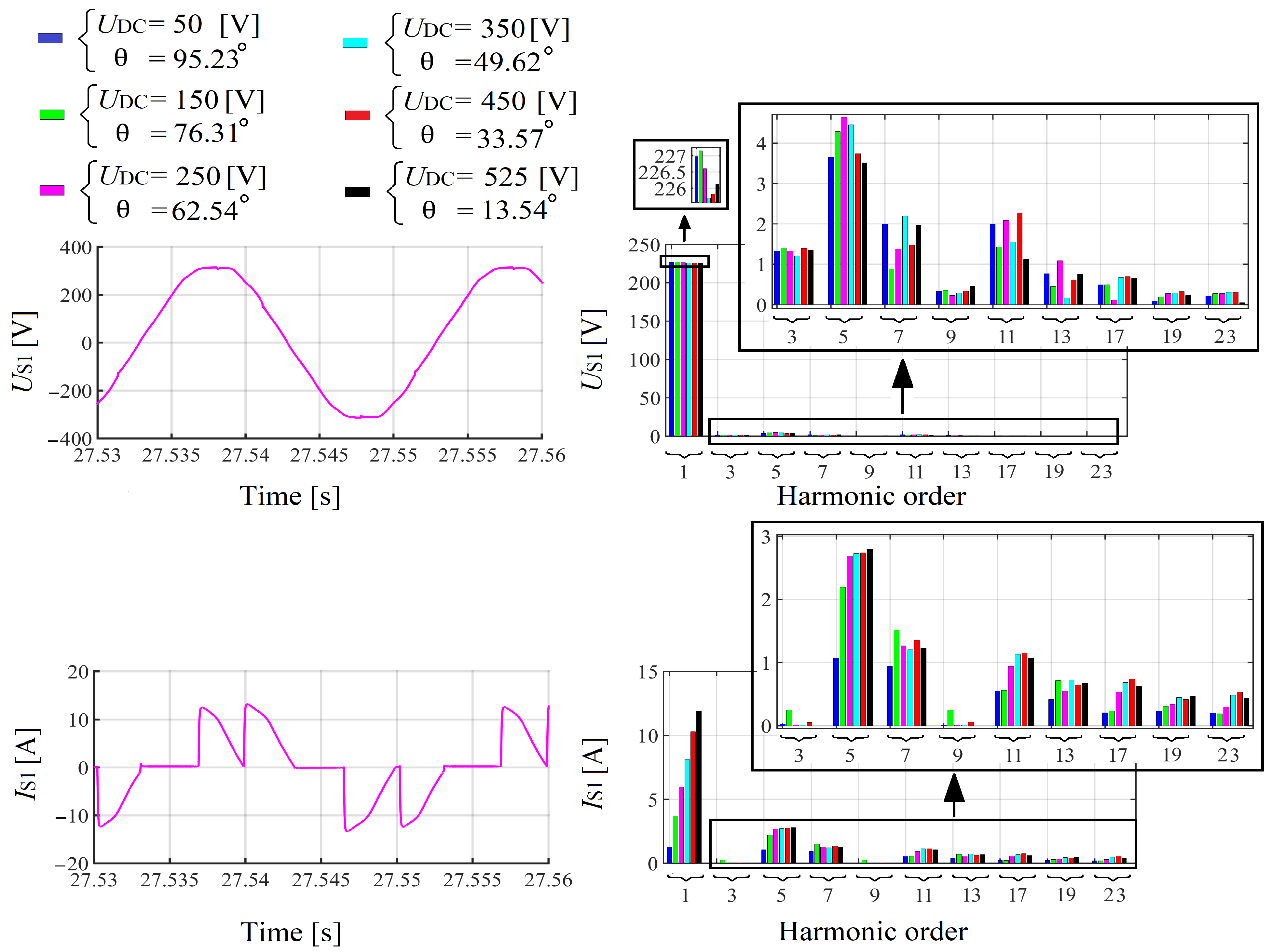
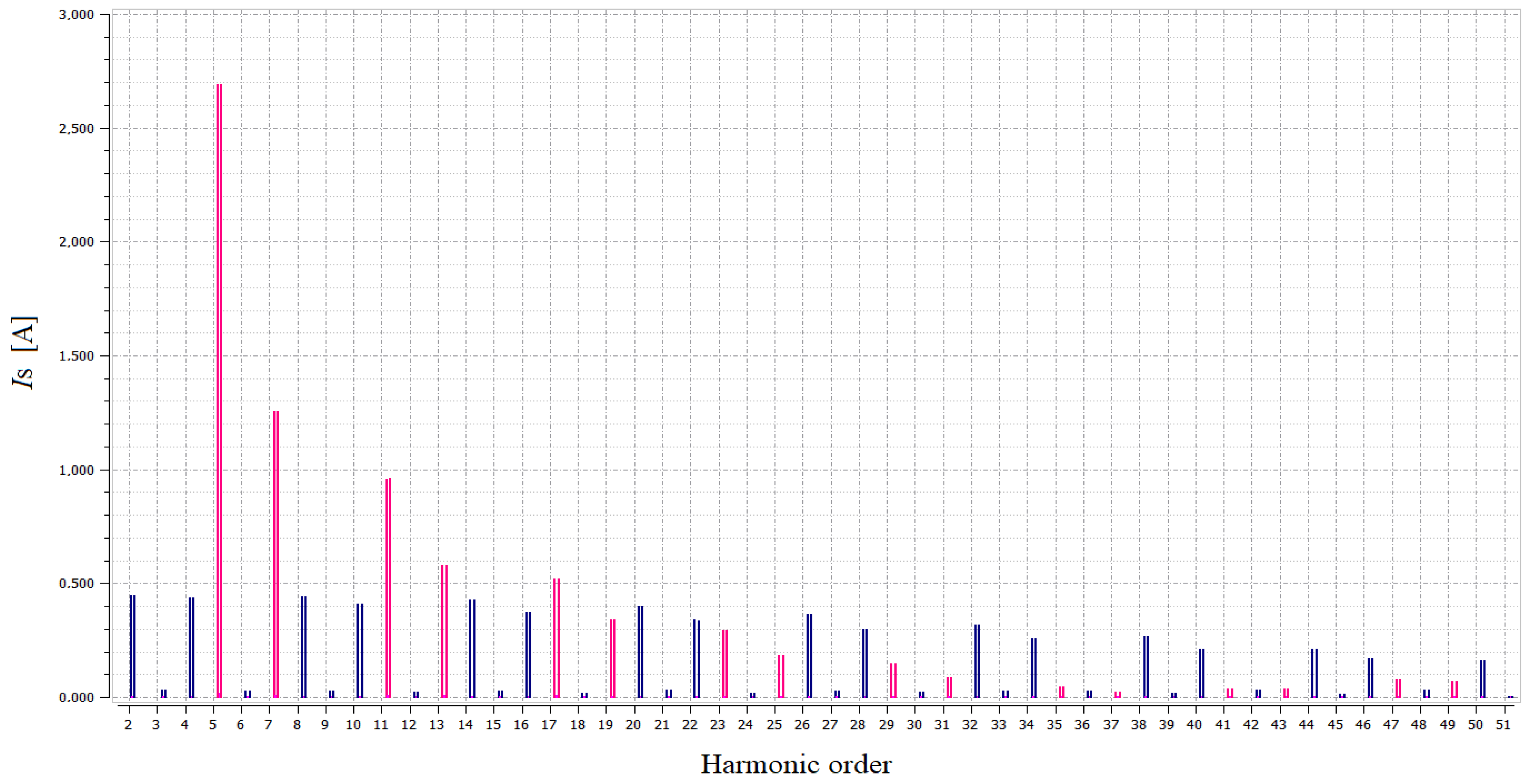
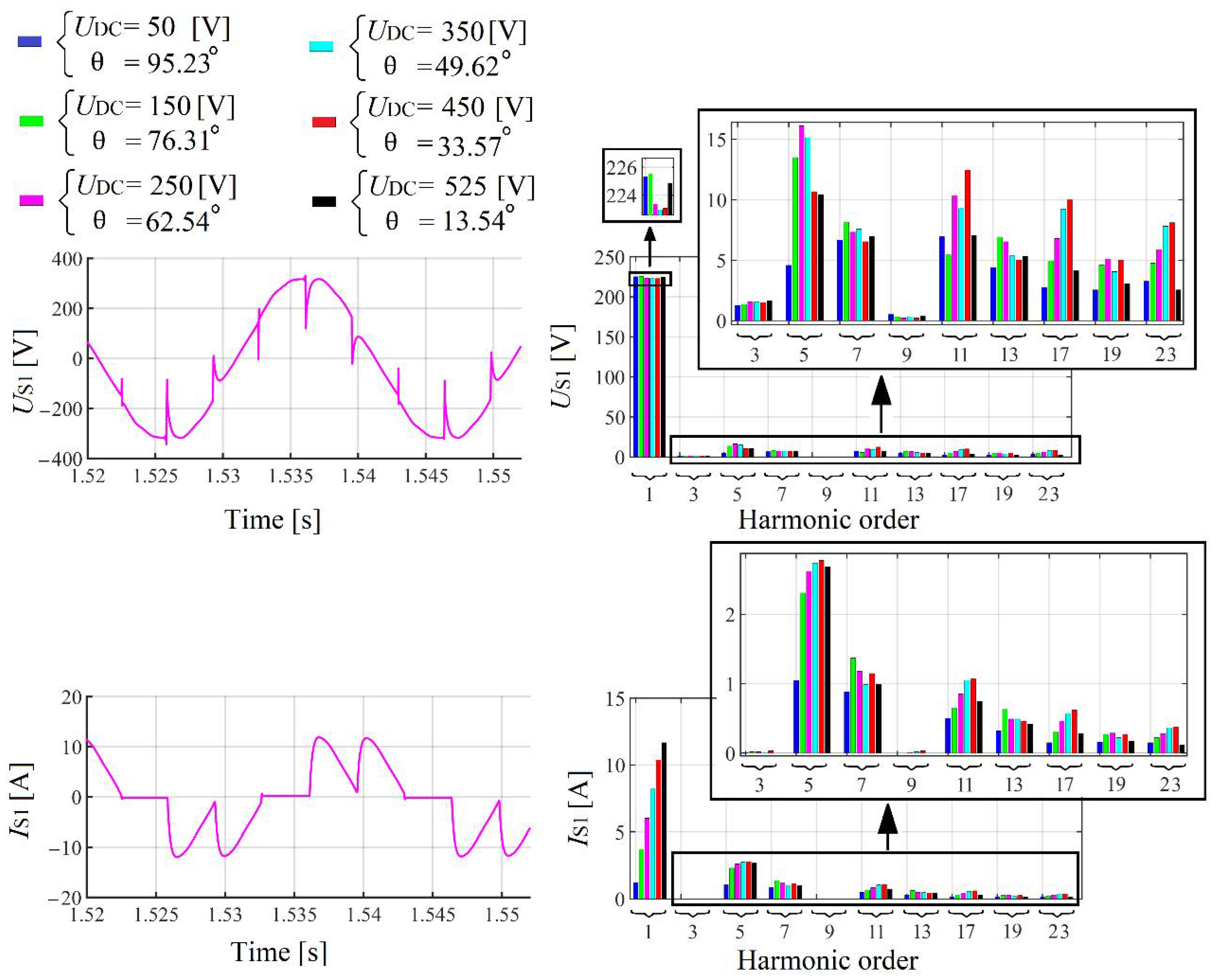
2.2.2. Investigation on the Change of the Amplitude of the Harmonics versus Rectifier Firing Angle

The spectrums in Figure 6 presents the behavior of the amplitude of the grid voltage and current harmonics when the rectifier DC voltage is increased. Concerning the amplitude of the grid voltage fundamental harmonic, it has slightly decreased with the increase in UDC (e.g., from 226.97 V (UDC = 50 V) to 226.13 V (UDC = 525 V)). The 5th harmonic has the highest amplitude for UDC equal to 250 V and the 7th harmonic for UDC to 350 V (Figure 6).
An example of a measured grid current spectrum (θ = 62.54°) is presented in Figure 7. Observing that spectrum, it can be noticed that with the increase in harmonic order, some of the non-characteristic harmonics present higher amplitude than the characteristic harmonics.
Figure 8, Figure 9 and Figure 10 present the behavior of the RMS value of the 1st, 5th, and 7th harmonics current and voltage, respectively, with the rectifier firing angle increase. The comparison between characteristics obtained from the laboratory model and those obtained from the simulation is also presented.
Figure 8a,b represent the voltage and current (fundamental harmonic) versus rectifier firing angle, and Figure 8c,d represent the voltage and current (fundamental harmonic) versus rectifier DC voltage. The difference observed between the simulated grid voltage and the laboratory grid voltage (Figure 8) is due to the fact that in the case of simulation, the supply grid voltage was not distorted (pure sinusoidal waveform before the load connection), whereas, in the case of the laboratory, the supply grid voltage was already distorted before the load connection because of other devices which are continually connected and disconnected (the real electrical grid works continuously).
The RMS values of the grid voltage and current 5th harmonic measured in the laboratory (Figure 9a,c) are different from those of the simulation (Figure 9b,d) because, before the rectifier connection, the laboratory PCC voltage contained already the 5th harmonic (see spectrum Figure 3b). The same phenomenon is observed for the 7th harmonic (see Figure 10).

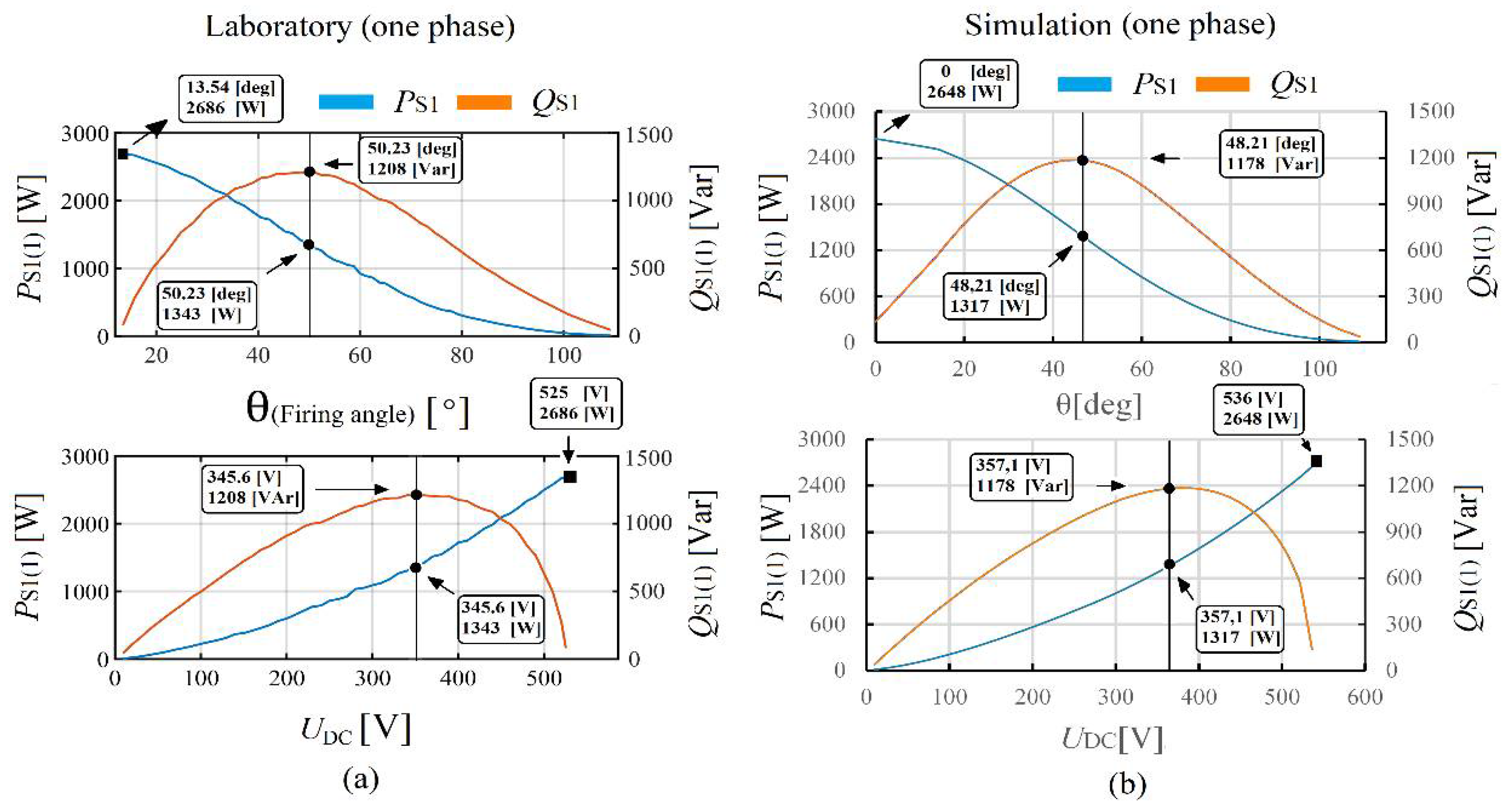
2.2.3. Investigation on the Load Active and Reactive Power versus Rectifier Firing Angle

In this particular case study, it is important to notice the firing angle to which the maximum or minimum fundamental harmonic reactive or active power is achieved. The PCC active and reactive powers (fundamental harmonic) versus rectifier firing angle and versus rectifier DC voltage are shown in Figure 11a (laboratory) and Figure 11b (simulation). The active power decreases with the firing angle increase and increases with UDC increase (Figure 11a). The reactive power characteristic has achieved its maximum (1208 Var) for a θ equal to 50.23° and UDC equal to 345.6 V (Figure 11a).

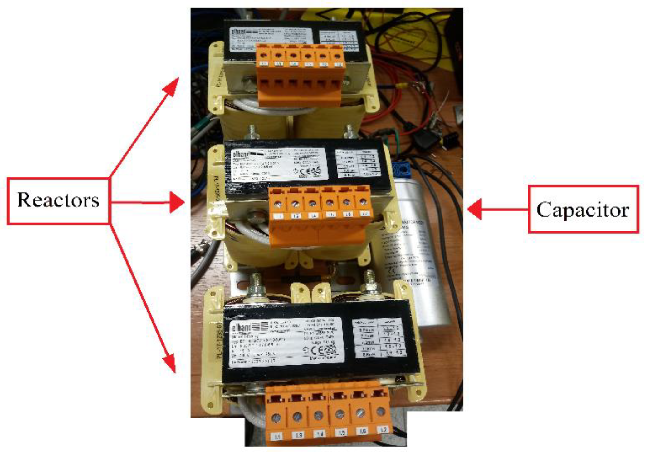
2.3. Design of the Single-Tuned Filter in the Laboratory

After performing the investigation on the parameters of the electrical network and load, the single-tuned filter was designed. The studies were based on the factors having an influence on the PHFs work efficiency and performance, such as the tolerance of the filter elements (e.g., reactor and capacitor), the electrical grid equivalent impedance of the harmonic to be eliminated, and the harmonics contained in the spectrum of the supply grid voltage (when no load is connected). The detuning of the single-tuned filter was also investigated.

2.3.1. Computation of the Single-Tuned Filter Parameters

According to the information obtained from the investigation on the electrical network and load: the lowest generated characteristic harmonic (in terms of harmonic order) after the fundamental harmonic is the 5th harmonic (see Figure 6), the computed equivalent impedance of the electrical grid 5th harmonic (ZS(5)) is around 49.5 mΩ (see Figure 2b), and the highest load reactive and active power (one-phase) are, respectively, around 1208 Var (inductive) and 2686 W (see Figure 11a). The filter equivalent circuit is presented in Figure 12a and the expressions used to compute its parameters are shown in Figure 12b.
The single-tuned filter used to mitigate the grid current 5th harmonic order is tuned to the frequency (fre = 245 Hz, nre = 4.9) a bit lower than the frequency of 250 Hz (because of the aging of the filter elements). The computed parameters of the filter are presented in Table 1 (one-phase). The filter reactive power value 1000 Var was chosen to investigate in the laboratory the non-compensation, compensation, and over-compensation mode of the power system after the change of the rectifier firing angle.
Comparing the 5th harmonic equivalent impedance of the electrical grid (ZS(5) = 49.5 mΩ) to the one of the filters (Zf(5) = 450 mΩ—see Table 1), it can be noticed that the 5th harmonic equivalent impedance of the filter is almost nine times higher than the one of the grid, which allows concluding that the filter will be less efficient on the 5th harmonic mitigation at the grid side. The simulated impedance versus frequency characteristic of the filter is presented in Figure 13.

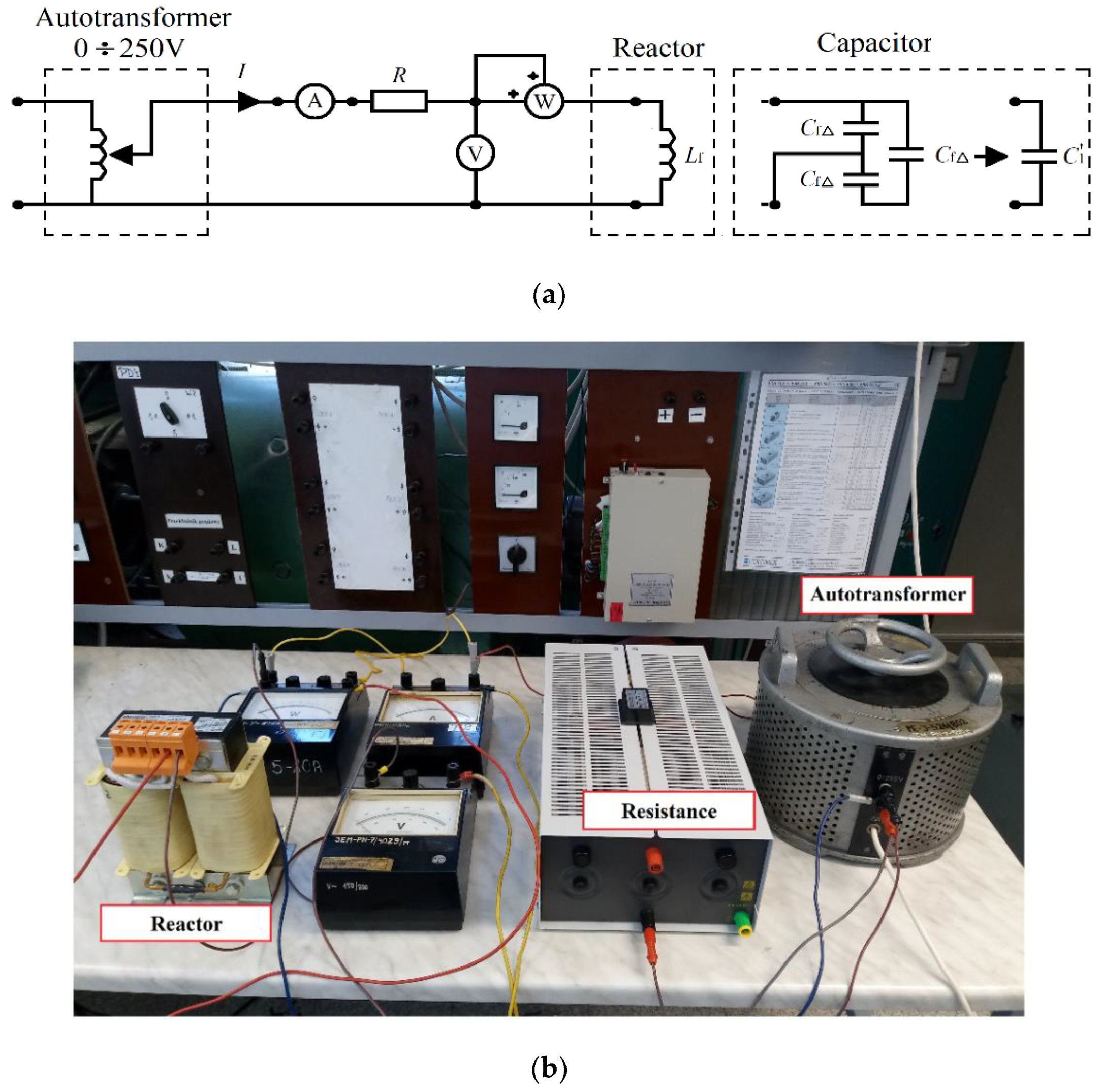
2.3.2. Measurements of the Single-Tuned Filter Parameters in the Laboratory: Verification of the Manufacturer Tolerance

After theoretically computing the filter parameters (see Table 1), the filter elements were obtained from the manufacturer (see Figure A1 in Appendix A). The technical data of the filter reactor and capacitor are presented in Table 2.
The core reactors with many terminals (Figure A1 in Appendix A) were chosen with the goal of investigating the filter detuning phenomenon in the laboratory. Firstly, the reactor inductances were theoretically computed, increasing the inductance 7.3 mH by ±5% and ±10%. The obtained theoretical inductances (8.03 mH, 7.665 mH, 6.93 mH, and 6.57 mH) were sent to the producer. The technical data of the physical reactors (8.03 mH, 7.7 mH, 7.3 mH, 7.0 mH, and 6.6 mH—see Table 2) were a bit different from the theoretical ones.
The obtained capacitor bank from the manufacturer is in delta connection with a capacitance of 19.2 µF and 966.66 Var for each capacitor. The total reactive power of the three-phase capacitor bank is around 2.9 kVar for 400 V phase to phase. The capacitor bank capacitance (Cf∆) in the technical data in Table 2 is according to the theoretical computation.
Because of the manufacture tolerance, the parameters of the filter elements were verified in the laboratory using the ammeter–voltmeter–wattmeter method (this method is very common and can be used under any condition in the industries (see Figure A2b in Appendix A). The Equations (A1) and (A2) in Appendix A were used for the computation (see Table 3). The equivalent circuit of the laboratory model in which the filter parameters were verified is presented in Figure A2a (see Appendix A).
The computed filter parameters (Lf, Cf∆) in the laboratory are shown in Table 3. It can be noticed that these parameters are a little bit different from the ones of the manufacturer but are within the manufacturer’s tolerances (±10% for the reactors and −5% to 10% for the capacitor (see Table 2).
The filter resonance frequencies (fre) data measured in the laboratory through the programmable voltage source in Figure 14 are presented in Table 4. The recorded data were obtained after each 50 Hz, but around the resonance frequency, the interval of 10 Hz was used (Chroma [66]). The single-tuned filter impedance versus frequency characteristic measured in the laboratory is presented in Figure 15.
In Table 4, the frequencies obtained from the manufacturer data are compared to the frequencies obtained from the computed data (Table 3) and to the measured frequencies (through the electrical circuit in Figure 14). It can be observed that the measured and computed resonance frequencies are almost the same, whereas the manufacturer frequencies are different from the measured frequencies (Table 4). The tolerance of the filter elements (capacitors and reactors) has an influence on the expected resonance frequency. For instance, in the case of the expected frequency of 245 Hz (nre = 4.9), the measured frequencies have shown: 238.5 Hz (nre = 4.77) (see Table 4 and Figure 15).
The real parameters (from the laboratory) of the single-tuned filter presented in Table 5 shows that the 5th harmonic equivalent impedance of the filter (Zf(5) = 1160 mΩ, see Table 5) is almost 23 times higher than the one of the electrical grids (ZS(5) = 49.5 mΩ). The filter will be less efficient on the 5th harmonic mitigation at the grid side.
Because of the manufacturer’s tolerance, it is very impotent to verify the parameters of the filter elements after their reception.

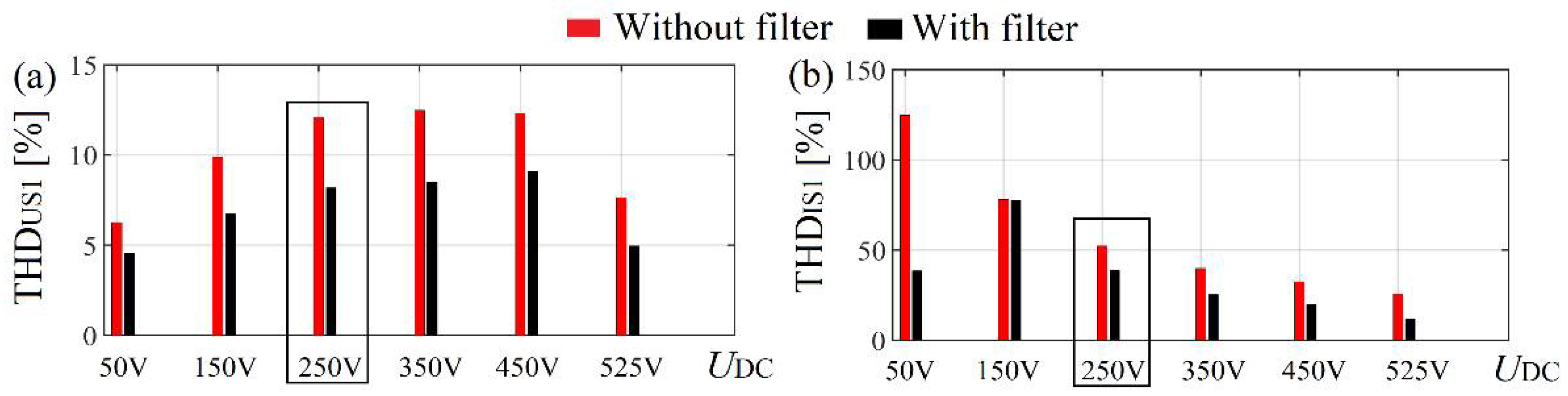
2.4. Laboratory Results after the Single-Tuned Filter Connection at the PCC

The equivalent circuit of the laboratory model in which the 5th harmonic filter was designed is presented in Figure 16 and the filter impedance versus frequency characteristic measured in the laboratory is presented in Figure 15. The parameters in Figure 16 were computed based on the measured parameters of Table 3.
Table 6 presents some parameters of the electrical system for different rectifier firing angle values after the filter connection. It can be noticed that the grid voltage presents the highest THD (THDUS1 = 2.24%) for UDC equal to 350 V (θ = 33.57°) and the lowest THD for UDC equal to 525 V (θ = 13.54°), whereas the grid current presents the highest THD (THDIS1 = 156.09%) for UDC equal to 150 V (θ = 76.31°) and the lowest THD (THDIS1 = 36.57%) for UDC equal to 525 V (θ = 13.54°). For the rectifier firing angle θ from 0° to 13.54° and from 76.31° to 95.23°, the electrical gird is overcompensated. For θ between 26.54° and 33.57°, the electrical grid reactive power is compensated. In this case study, the better fundamental reactive power compensation (e.g., QS1(1) = 49.58 Var) is when the rectifier firing angle is around 33.57°. The single-tuned filter power losses have increased with the decrease in firing angle.
Despite the filter presence in the electrical system, the grid current THD (THDIS1) is higher than the load current THD (THDIT1) (see Table 6). This increase in the grid current THD after the filter connection is due, on the one hand, (depending also on the firing angle value and taking into account the expression (3) used to compute that THD) to the reduction (because of the reactive power compensation) or amplification (because of the overcompensation) of the grid fundamental harmonic, and, on the other hand, to the amplification of some harmonics (e.g., 5th, 7th, etc.) at the electrical grid side (see also the current spectrum in Figure 17 compared to Figure 6).
The grid voltage and current waveforms together with spectrums after the 5th harmonic filter connection are shown in Figure 17. The waveforms and spectrums of the rectifier input current and the filter current are presented in Figure 18. The grid current spectrum in Figure 17 shows that the lowest amplitude of the 5th harmonic is obtained for UDC equal to 250V (θ = 62.54°) when the filter reactive power 966.6 Var is around the load reactive power 1048.1 Var. The filter current is more charged by the 5th harmonic than the other harmonics (see the spectrum of IT1 in Figure 18).
THD I = n = 2 50 I n 2 I 1
Comparing Figure 17 to Figure 6, it can be noticed that the grid voltage 5th harmonic amplitude has decreased after the filter connection (see also US1(5) in Figure 19b). The grid voltage waveform is improved after the filter connection (See THDUS in Figure 19a).
The change of the grid voltage 7th harmonic amplitude before and after the filter connection is presented in Figure 19c. For certain firing angles (e.g., 95.23°), the 7th harmonic amplitude is reduced at the grid side after the filter connection, and for others (e.g., 76.31°), it is amplified.
The filter work efficiency on the harmonic’s mitigation (from the 1st to the 23rd) is presented in Figure 20a. The amplification of some harmonics at the grid side after the filter connection can be observed (values higher the 100%, e.g., the 5th, 7th, etc.) for a certain value of θ. The grid current fundament harmonic is amplified (UDC equal to 50 V and 525 V) because of the overcompensation.
For UDC equal to 250V (θ = 62.54°), the single-tuned filter efficiency on the grid current 5th harmonic mitigation is around 80.74% (see Figure 20a—only 19.26% of 5th harmonic current generated by the load has flowed to the electrical grid). Figure 20a also shows that the filter efficiency on the 5th harmonic mitigation varies with the rectifier firing angle. For certain rectifier firing angles (e.g., 76.31° to 49.62°), the filter is more efficient on the 5th harmonic mitigation, and for others (e.g., 95.23°, 33.57°, and 13.54°), it is the source of 5th harmonic amplification. The behavior of the filter on the 5th harmonic mitigation is abnormal because, for each value of rectifier firing angle, the filter should be more or less efficient on the 5th harmonic mitigation at the grid side.
In Figure 20b, the amplitude of the 5th harmonic of the input rectifier current (IT(5)) is compared to the one of the grid currents (IS(5)) for different firing angle values. It can be noticed (as in Figure 20a) that for a θ equal to 95.23°, 33.57°, and 13.54°, the 5th harmonic amplitude is higher at the grid side than at the load side. For a θ equal to 76.31°, 62.54°, and 59.62°, that amplitude at the grid side is smaller than the load side.
For any value of thyristor bright firing angle, the filter should be able to mitigate the grid current 5th harmonic amplitude. Because of that abnormal behavior of the single-tuned filter on the 5th harmonic mitigation at the grid side (amplification of the 5th harmonic amplitude at the grid side for certain firing angles), some extra experiments are carried out and presented in the next part of this paper to bring more clarification.

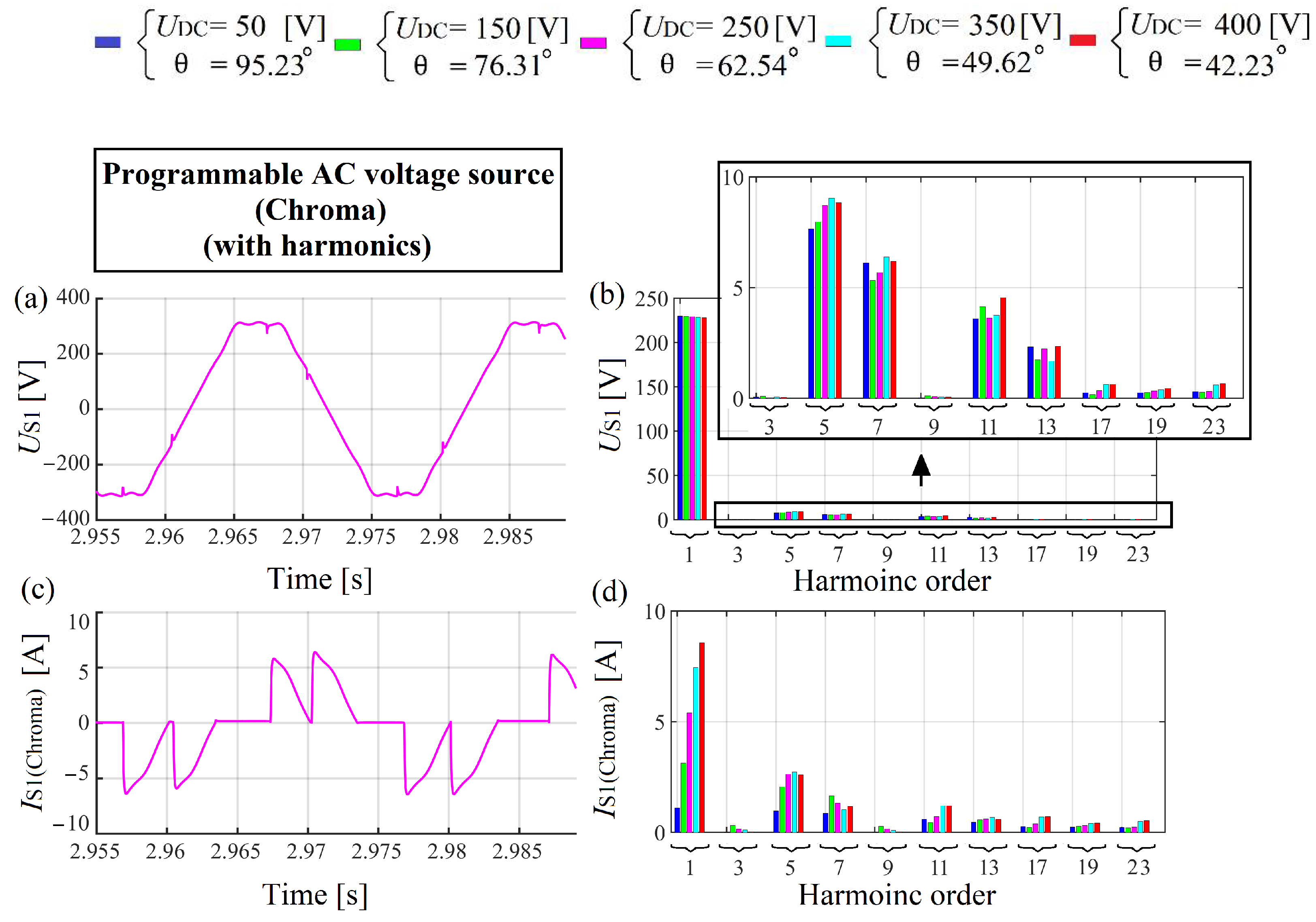
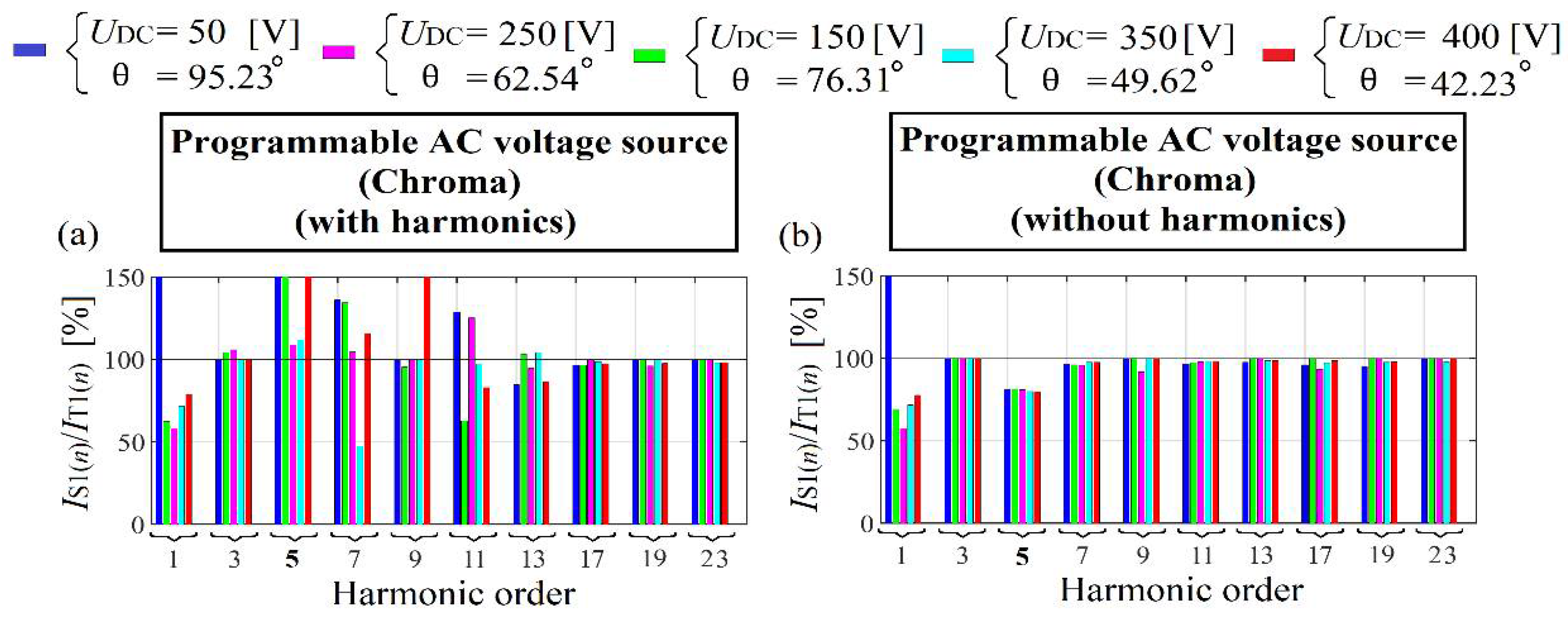
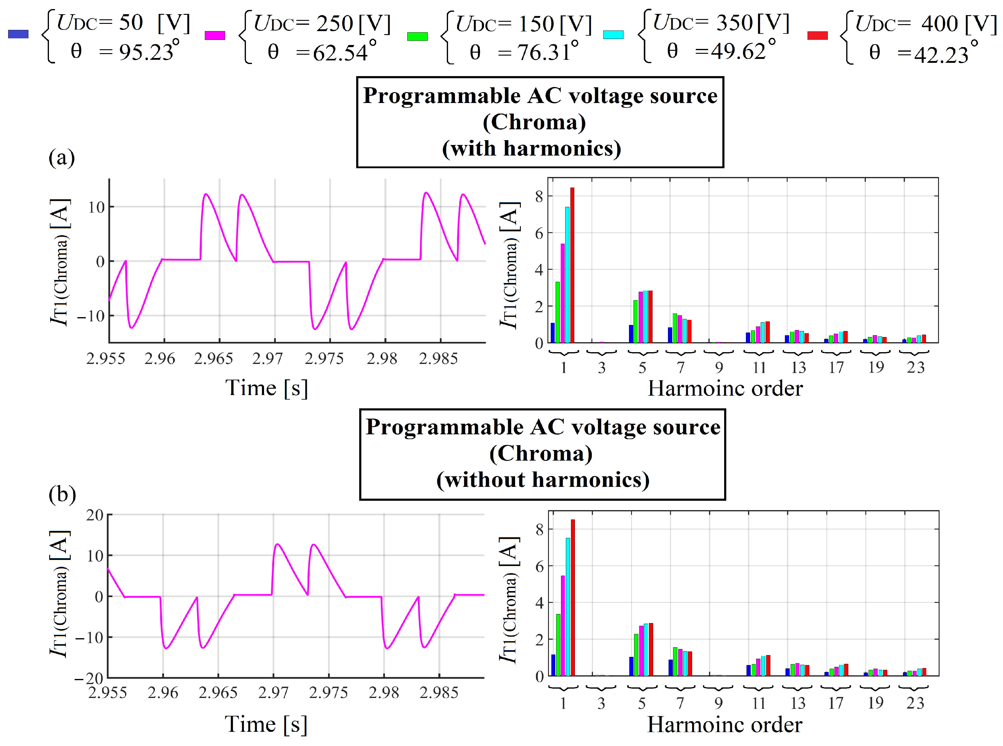
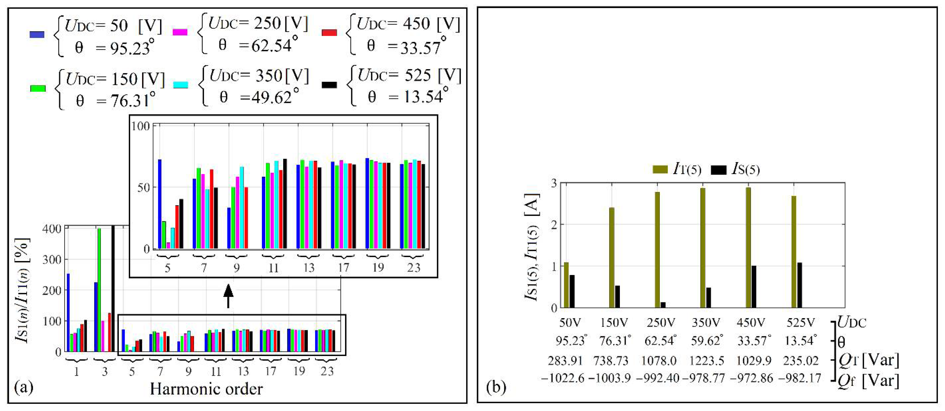
2.4.1. Experiments with Chroma to Clarify the Amplification of the 5th Harmonic at the Grid Side after the Filter Connection

The laboratory model (load plus filter) was disconnected from the electrical grid and supplied by the programmable AC voltage source (see Figure 21) with a cable of 0.11 Ω and inductance of 63.69 µH. Two types of experiments were carried out: in the first one, the programmable voltage source is the source of the fundamental harmonic as well as other harmonics such as the 5th, 7th, 11th, and 13th (see Figure 22a) (the programmable voltage source with harmonics represents the electrical grid with distorted supply voltage as presented in Figure 3). In the second one, it is the source of the fundamental harmonic only (without other harmonics (Figure 22b).
The amplitude of harmonics in the voltage spectrum in Figure 22a was chosen a bit higher than those in the electrical grid voltage spectrum presented in Figure 3b (when no load and filter were connected) to make the experiments clearer. The results obtained from the two experiments (after the filter connection) are presented in Figure 23, Figure 24, Figure 25, Figure 26, Figure 27, Figure 28, Figure 29, Figure 30 and Figure 31.
The voltage and current waveforms and spectrums measured at the PCC (without filter) when the load was connected at the programmable voltage source terminals are presented in Figure 23 (programmable voltage source with harmonics) as well as in Figure 24 (programmable voltage source without harmonics). Comparing the PCC voltage spectrum in Figure 23b to the one in Figure 24b (see also the waveforms in Figure 23a and Figure 24a), it can be noticed that the programmable voltage source with harmonics presents the highest amplitude of voltage harmonics at the PCC (e.g., 5th and the 7th). In the case of the programmable voltage source without harmonics, the harmonics observed in the voltage spectrum in Figure 24b are because of the voltage drop caused by each current harmonic (flowing from the load—see Figure 24c,d) on the cable wire connecting the load to the programmable voltage source. In the case of the programmable voltage source with harmonics, the harmonics observed in the voltage spectrum in Figure 23b (measured at the PCC) are the sum or subtraction between the provided voltage harmonics to the programmable voltage source (see Figure 22a and the voltage drop caused by the superposition of each current harmonic (flowing from the load as well as from the programmable voltage source—see Figure 24c,d) on the cable wire connecting the load to the programmable voltage source.
The waveforms and spectrums of the PCC voltage and current measured at the programmable voltage source input (see Figure 21) after the filter connection are presented in Figure 25, Figure 26, Figure 27 and Figure 28. The amplitudes of the 5th harmonic voltage and current at the input of the programmable voltage source with harmonics (see Figure 25b,d) is higher than in the case of the programmable voltage source without harmonic (see Figure 26b,d). The voltage and current waveforms are presented in Figure 25a,c and Figure 26a,c. The current spectrum in Figure 25d) shows that for UDC equal to 250V (θ = 62.54°), the 5th harmonic has the smallest amplitude as in the case of the grid current spectrum presented in Figure 17.
The load (IT) and filter (If) current waveforms and spectrums are respectively presented in Figure 27a,b and Figure 28a,b. Comparing Figure 27d and Figure 28d, it can be observed that in the case of the programmable source with harmonics, the amplitudes of current harmonics (e.g., 5th, 7th, 11th, and 13th) flowing through the filter are higher than in the case of the programmable voltage source without harmonics. It is due to the fact that apart from the current harmonics filtered by the filter, other current harmonics are flowing from the programmable voltage source side to the filter (case of the programmable voltage source with harmonics).
The filter efficiency spectrum in Figure 29a clearly shows that in the case of a programmable voltage source with harmonics, the amplitude of the 5th harmonic current is amplified at the programmable voltage source input (values above 100%), whereas in the case of programmable voltage source without harmonics, is it partially mitigated (see Figure 29b—no amplification of the 5th harmonic).
In Figure 30a,b, the amplitude of the 5th harmonic current measured at the thyristor bridge input (IT1(5)) is compared to the one measured at the Chroma voltage source input (IS1(Chroma)(5)). In the case of the Chroma voltage source with harmonics (see Figure 30a), the amplitude of the 5th harmonic current at the Chroma input side is higher than at the rectifier input side. The 5th harmonic amplification at the Chroma input side is because of the filter connection, which has attracted to him the 5th harmonic current flowing from the programmable voltage source side.
In the case of the Chroma voltage source without harmonics (see Figure 30b), the current amplitude of the 5th harmonic is not amplified at the Chroma voltage source input, but it is partially mitigated due to the fact that the filter 5th harmonic equivalent impedance (Zf(5) = 1.16 Ω—Figure 16) is almost eight times higher than the 5th harmonic equivalent impedance of the Chroma cable (ZCable(5) = 0.148 Ω). At the input of the programmable voltage source without harmonics, there is a part of non-filtered 5th harmonic current, whereas, at the input of the Chroma voltage source with harmonics, there is not only a part of non-filtered 5th harmonic but also a part of the 5th harmonic current flowing from the Chroma voltage source.
For any rectifier firing angle in Figure 30c, the THD of the current measured at the input of the Chroma voltage source with harmonics (THDIS1) is higher than the current THD measured at the load input (THDIT1). Almost the same situation is observable in Figure 30d (Chroma voltage source without harmonics), except for a θ equal to 95.23°.
The performed experiments can allow us to conclude that the amplification of the current amplitude of the 5th harmonic (for certain rectifier firing angle) at the electrical grid side as presented in the spectrums of Figure 20, was because of the 5th harmonic current flowing from the grid to the filter (which presented a small impedance for that current harmonic). In this case study, it can be noticed that the single-tuned filter (after its connection) has absorbed more 5th harmonic current from the grid side than from the load side, whence the amplification of that harmonic at the grid side. Another problem that should be highlighted after the above experiments is the partial mitigation of the amplitude of the 5th harmonic current at the Chroma voltage source input.
So far, it has been clearly demonstrated and presented the influence of the gird supply voltage distortion and grid impedance of the harmonic to be eliminated on the PHF work efficiency. In the case study presented in this paper, the proposed solution to mitigate the influence of the electrical grid on the PHF work efficiency is the use of an additional line reactor between the point of laboratory model connection and the PCC.

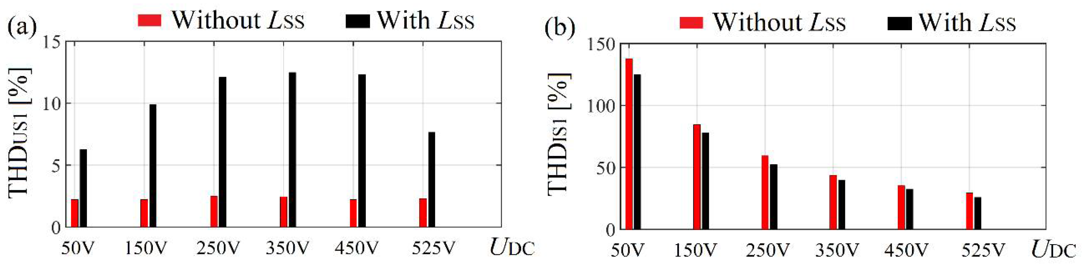
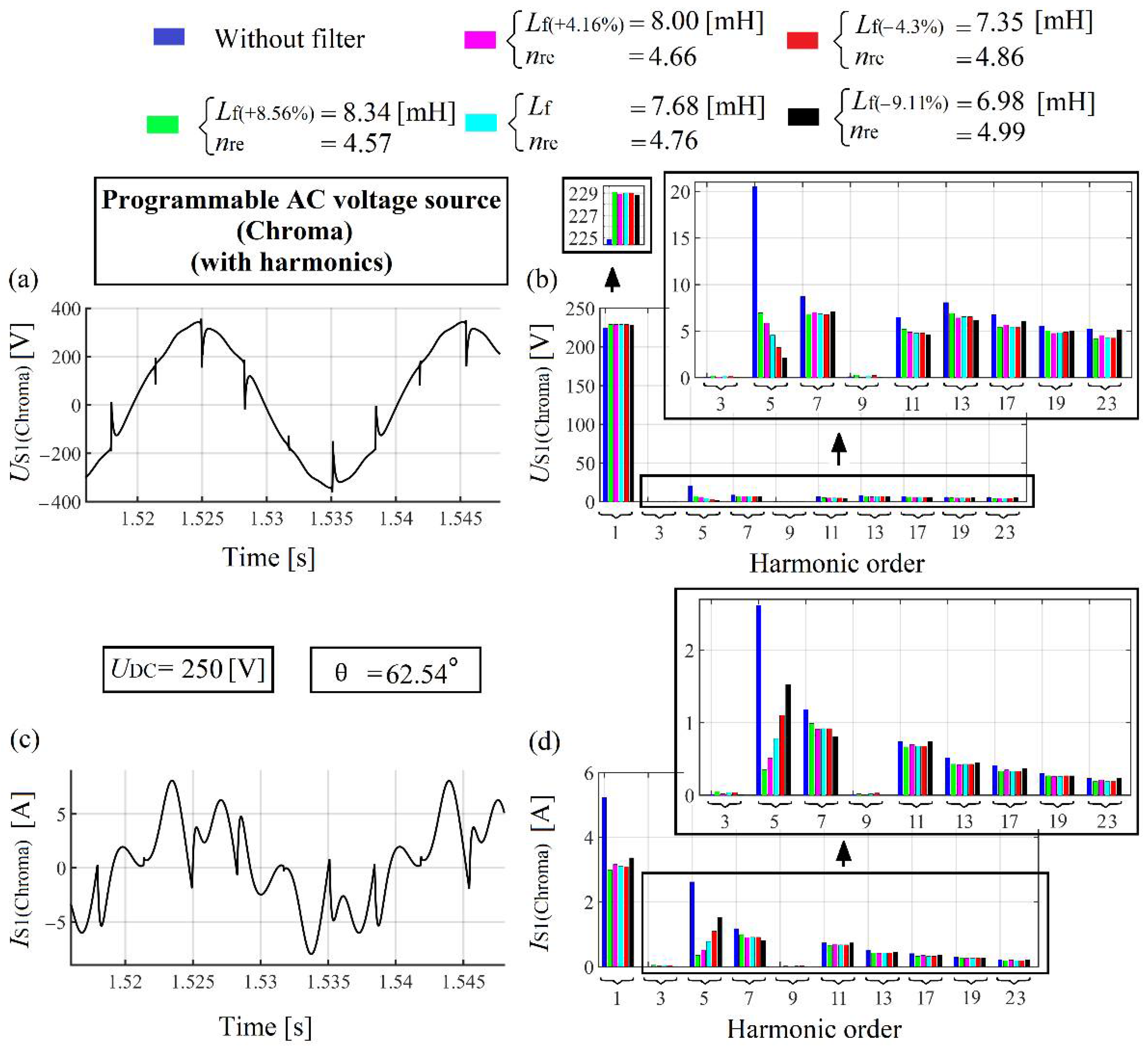
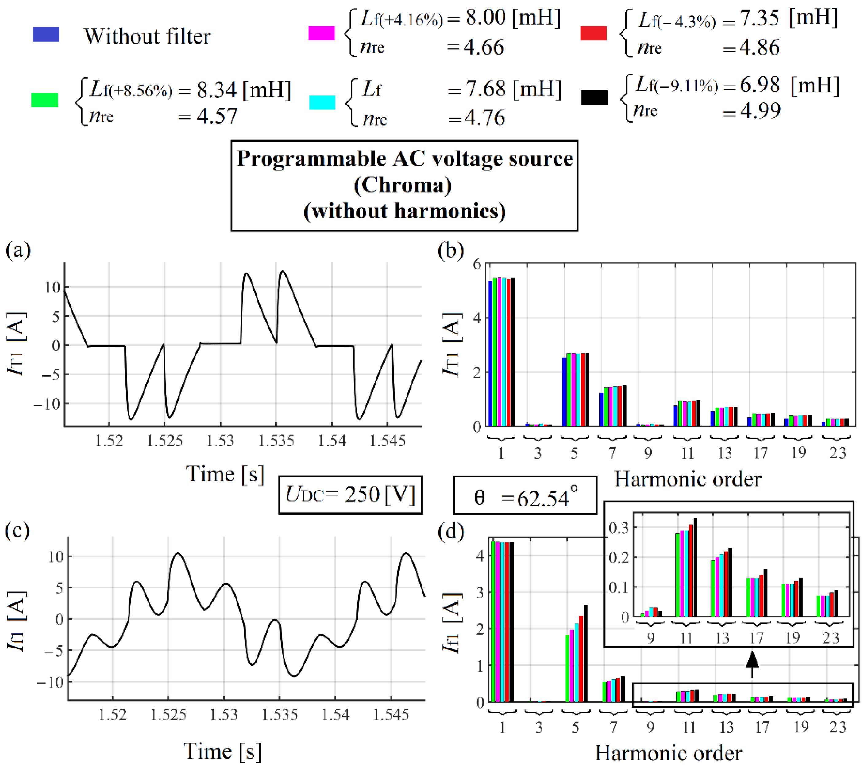
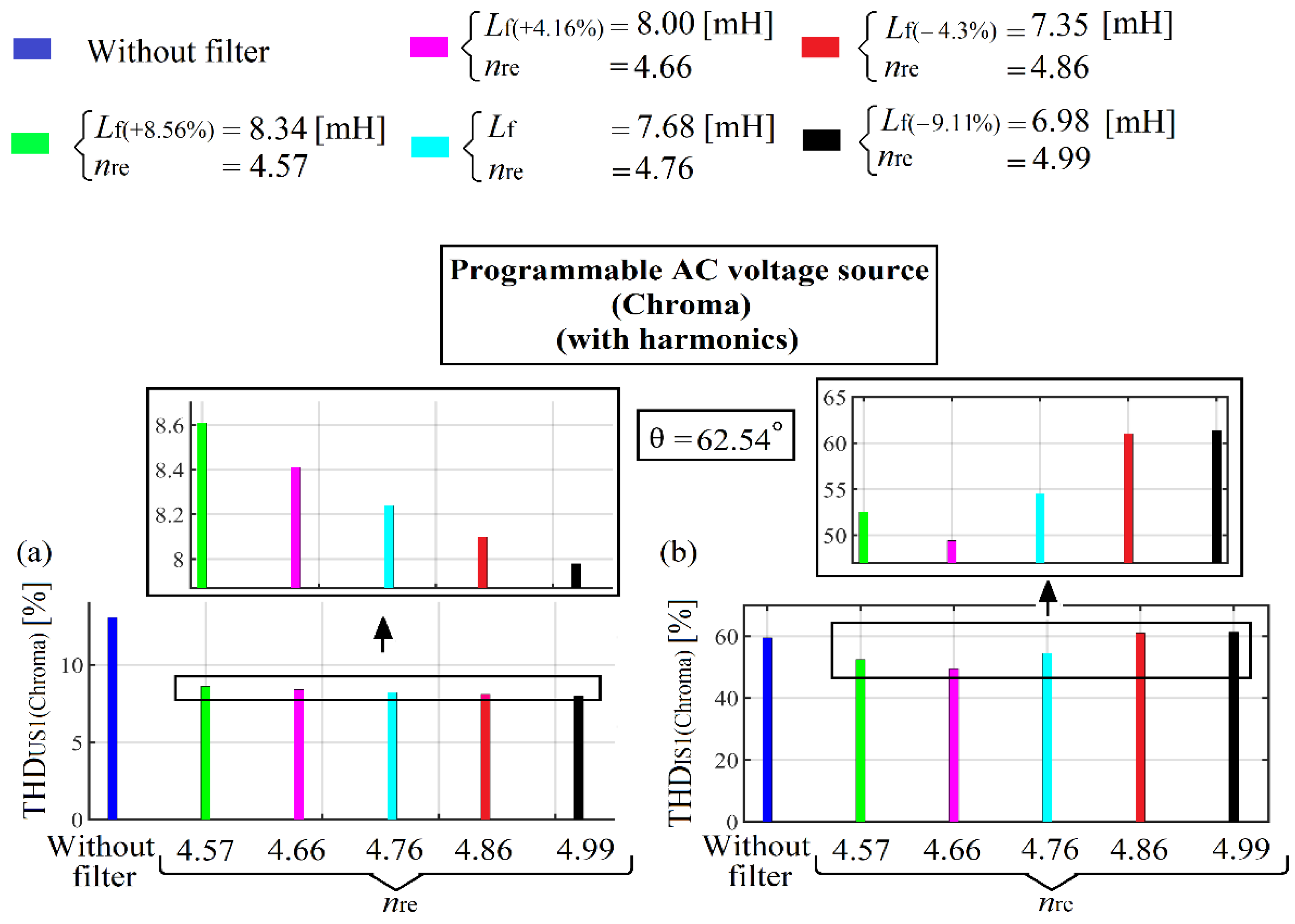
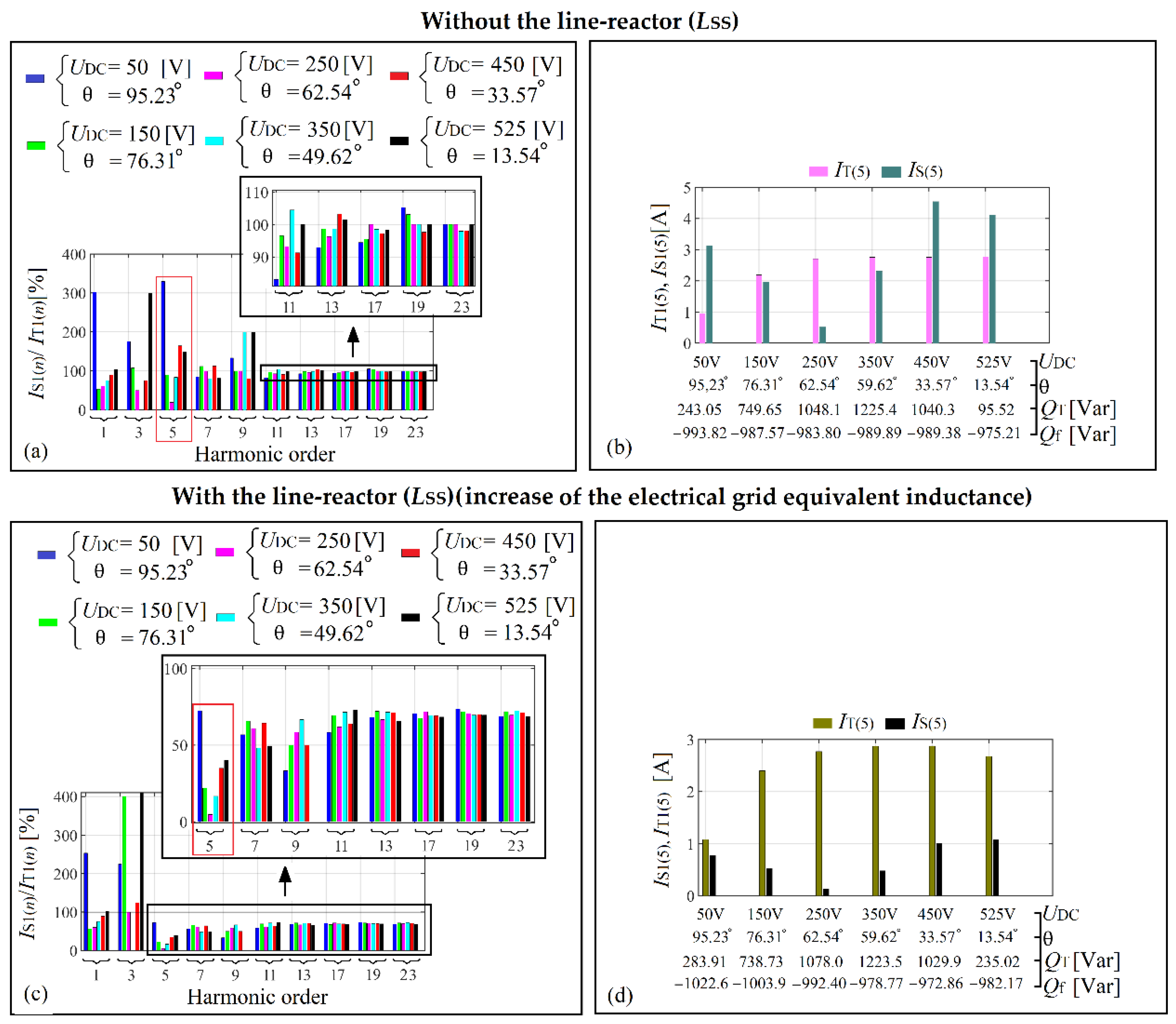
2.4.2. Experiments with the Additional Line Reactor to Improve the Filter Work Efficiency Using the Programmable AC Voltage Source (Chroma)

In this investigation, the line reactor (LSS–see Figure 31) is used, on the one hand, to mitigate the amplitude of the 5th harmonic current flowing from the Chroma voltage source to the filter (in the case of the programmable voltage source with harmonics). On the other hand, it is also used to increase the 5th harmonic equivalent impedance of the cable (connecting Chroma to the PCC) so that the efficiency of the filter on the 5th harmonic mitigation at the Chroma voltage source input will increase. In Figure 31, it can be noticed that the equivalent impedance of the filter (Zf(5)) is four times smaller than the one of the Chroma cable and line reactor added together (ZLSS(5)+ (ZCable(5)). In Figure 32a,b, the PCC voltage waveforms and spectrums are compared, and in Figure 33a,b, it can be observed the current waveforms and spectrums measured at the Chroma voltage source input. The filter current waveforms and spectrums are shown in Figure 34a,b. The load current parameters can be seen in Figure 35a,b.
Comparing the filter efficiency presented in Figure 29a,b (case without the line reactor LSS) to the one presented in Figure 36a,b (case with LSS), it can be noticed that the use of the additional line reactor LSS has improved the filter work efficiency on the mitigation of the 5th harmonic as well as higher harmonics at the Chroma voltage source input (Figure 36a,b).
Figure 37a,b shows that he amplitude of the 5th harmonic current at the programmable voltage input is better mitigated in the case where the line reactor is considered than in the case where it is not considered (see Figure 30a,b). Figure 37c,d in comparison to Figure 30c,d presents lower Chroma input current THD. With the additional line reactor LSS connected in the power system, the filter power losses (fundamental harmonic) have little increased (see Figure 38a,b).
The above experiments with the programmable voltage source have clearly shown that an additional line reactor connected between the PCC and the laboratory setup (load plus filter) can efficiently improve the passive filter work efficiency. Such of connection also has some disadvantages, which is discussed in the following section.

2.5. Increase in the Electrical Grid Equivalent Inductance (Short Circuit Power Decrease)

Coming back to the electrical grid system as the power source for the laboratory model, the line reactor LSS is firstly connected between the PCC and the grid (without filter), as presented in Figure 39. Such of connection seen from the PCC reduces the grid short-circuit power and increases the grid inductance. The goal is to increase the electrical grid equivalent impedance of the harmonic to be eliminated (the 5th harmonic).
In Figure 39, it can be noticed that after the line reactor connection, the grid equivalent impedance of the 5th harmonic (see from the PCC) has increased from 49.5 mΩ to 4.62 Ω. Since the line reactor LSS is now considered as a part of the grid, the 5th harmonic equivalent impedance of the electrical grid is around 4.67 Ω (see Figure 39).
Table 7 presents the active and reactive power as well as the DPF measured at the PCC for different rectifier firing angles.
Comparing the PCC voltage waveforms and spectrums in Figure 40 to those in Figure 6 (when the line reactor was not connected), it can be noticed that with the increase in the grid inductance using the additional line reactor (LSS), the PCC voltage is more distorted by commutation notches and the amplitudes of the harmonics have increased (Figure 40). The grid current waveforms and spectrums are presented in Figure 40 and there is no significant change in the amplitudes of the harmonics after comparison to the case without LSS in Figure 6.
The comparison between the PCC voltage and current THD as well as fundamental harmonic amplitude before and after the line reactor connection is presented in Figure 41 and Figure 42, respectively. The THD of the grid voltage has increased (Figure 41a), whereas its fundamental harmonic has decreased (Figure 42a) after the line reactor connection. The grid current THD has decreased (the line reactor has worked as a filter) (Figure 41b) and the fundamental harmonic is almost the same (Figure 42b) with the line reactor presence.
On the one hand, the additional line reactor has increased the electrical grid equivalent impedance of harmonic to be eliminated and reduced the amplitude of current harmonics. On the other hand, it has increased the PCC voltage distortion (THD) and reduced the amplitude of the PCC voltage fundamental harmonic.
Figure 43 shows that the depth of voltage commutation notches is more accented with the line reactor inductance increase. The higher the line reactor inductance (e.g., LS + L + LSS), the more dipped are the voltage commutation notches (see UT). The voltage waveform at the PCC (US) is less distorted by commutation notches than the one at the rectifier input (UT) (Figure 43) because, at the PCC, the inductance LS is small. The commutation dip observed on the voltage U (Figure 43) is because of the voltage swell on the reactor’s voltage (LS + L).

Connection of the Single-Tuned Filter at the PCC after the Increase in the Electrical Grid Inductance

The laboratory model is shown in Figure 44 and its equivalent circuit in Figure 45. The 5th harmonic grid equivalent impedance (ZS(5) + ZLSS(5) = 4.67 Ω) is around four times higher than one of the filters (Zf(5) = 1.16 Ω, Figure 45). At the PCC, the grid inductance is almost 93.33 times higher than before the line reactor connection.
The parameters in Table 8 were registered by increasing (with the filter connected) the rectifier DC voltage from 0 to 525 V. The better grid fundamental harmonic reactive power (QS(1)) compensation is observed for θ = 26.54° (UDC equal to 250 V, Table 8). With the line reactor connected in the electrical system as presented in Figure 45 and for any value of the rectifier firing angle, the THD of the electrical grid current (THDIS1) is smaller than the one at the rectifier input (THDIT1, Table 8), which is totally different from the situation when the line reactor was not connected (see Table 6).
The PCC voltage waveform and spectrum are presented in Figure 46. Compared to the case without line reactor LSS (see voltage spectrums in Figure 17), the voltage spectrum in Figure 46 presents the highest amplitude of 7th, 11th, 13th, 17th, 19th, and 23rd (see also Figure 43), and higher harmonics (because of the commutation notches depth increase) as well as the best reduction in the 5th harmonic amplitude in the grid voltage.
The grid current waveforms and spectrum are constituted by Figure 46 (the lowest value of the 5th harmonic amplitude is obtained when the thyristor bridge firing angle was set to 62.54° (UDC = 250 V). Comparing the grid current spectrum in Figure 46 to the one in Figure 40 (grid with line reactor without filter), it can be observed that the 5th harmonic amplitude has considerably decreased after the filter connection.
Figure 47 presents the waveform and spectrum of the filter current and input rectifier current. On the top of that figure, an example of the measured current complex form is presented.
With the increase in grid inductance and for any DC rectifier voltage (Figure 48a), the filter is more efficient (when compared to the case without LSS in Figure 20a) on the 5th and higher harmonics reduction (values below 100%—Figure 48a). The amplification of the 3rd harmonic (grid side) observed in Figure 48a is due to its presence near the parallel resonance frequency occurring between the filter capacitor and the grid inductance.
The comparison between the 5th harmonic generated by the load (IT(5)) and the one flowing to the electrical grid (IS(5)) is presented in Figure 48b. For any firing angle, there is non-grid side 5th harmonic amplification as in Figure 20b. The line reactor has increased the filter efficiency in terms of 5th and higher harmonic mitigation.
A comparison example of the grid voltage and current spectrum and THD before and after the filter connection (with the line reactor) is considered in Figure 49 and Figure 50. For almost all rectifier firing angles, the grid current and voltage THD have decreased after the filter connection (Figure 50).
The power system impedance versus frequency characteristic seen from the load input (from the simulated model) is presented in Figure 51. It can be observed that the series (238 Hz) and parallel (201.7 Hz) resonances have appeared below the 5th harmonic frequency. In Figure 51, the series resonance is the filter resonance, and the parallel resonance is the resonance between the filter capacitor and the grid inductance (LS + LSS). The frequency 217.4 Hz represents the neutral frequency. All the harmonics having their frequency near the parallel resonance frequency can be amplified as in the case of the 3rd harmonic in Figure 48a.
The use of an additional line reactor between the PCC and the filter has improved the filter work efficiency on the 5th and higher harmonics mitigation at the grid side (Figure 48).

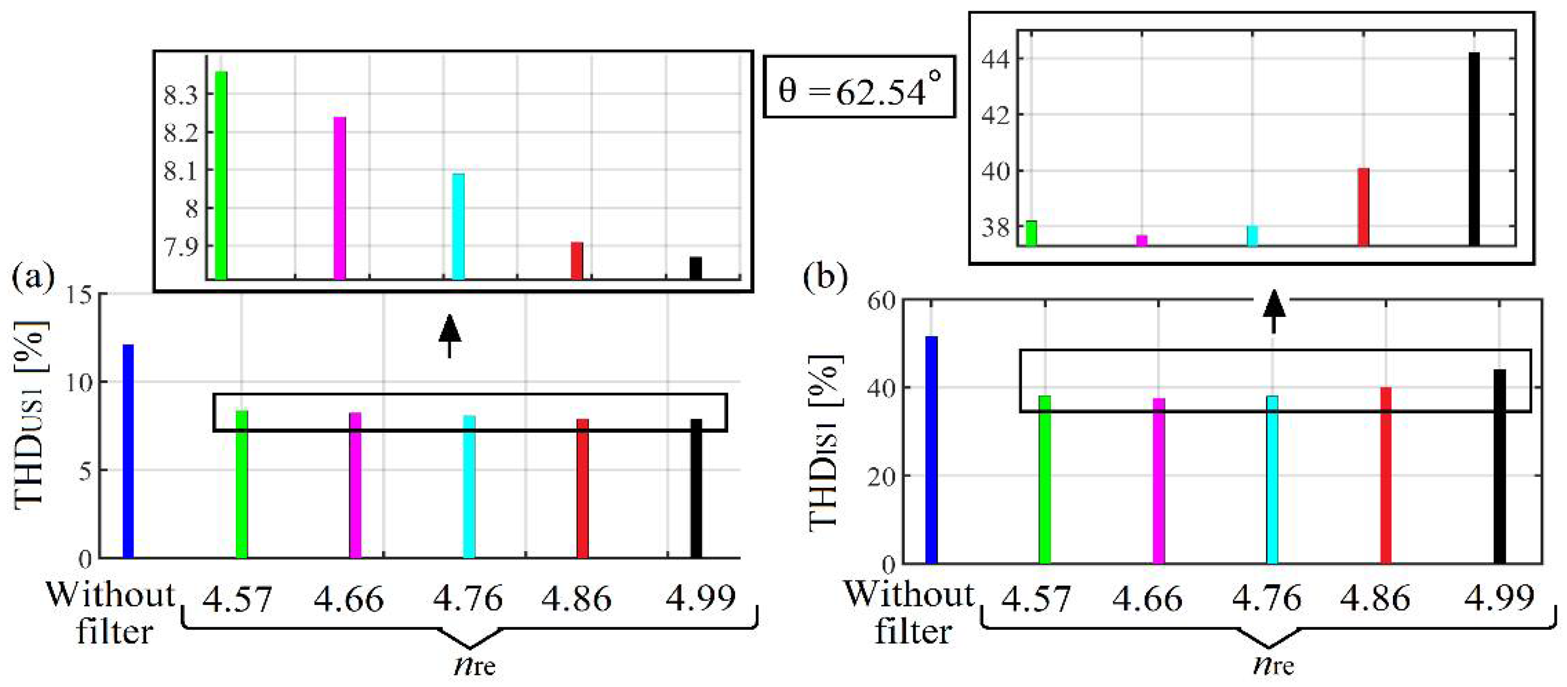
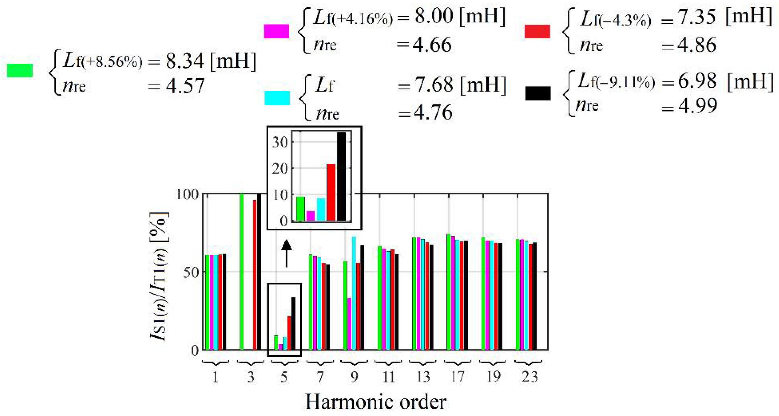
2.6. Detuning of the Single-Tuned Filter

In the following part of this paper, we present the case study in which the single-tuned filter is tuned to different resonance frequencies. The investigation goal was to present the influence of the filter detuning phenomenon on its filtration efficiency.
The PHF detuning phenomenon is characterized by the increase or decrease in the tuning frequency (resonance frequency) over time. This phenomenon can be caused by the variation of the PHF parameters over time or the voltage fundamental harmonic frequency change at the point of PHF connection. The variation of the filter parameters (increase or decrease in the inductance or capacitance value) can be caused by their aging (mostly the capacitor), the atmospheric conditions (temperature, humidity, etc.), or their damage. The filter inductance value decrease can take place in the event such as an inter-turn short circuit in the reactor (this condition leads to reactor damage). The change in capacitor capacitance is mainly caused by the work temperature increase. The capacitor’s aging reduces their capacitance over time [67,68]. It is very important to take into account the detuning phenomenon while designing the PHFs. In practice, it is advised to tune the PHF on the resonance frequency a bit lower than the frequency of the harmonic to be mitigated. In [59], there are formulated recommendations on the parameters that should be considered while choosing the PHF resonance frequency.
To investigate the detuning phenomena in the laboratory, the single-tuned filter reactor was designed with many terminals (see Figure 52). Each terminal represents one filter resonance frequency when connected to the capacitor. In Figure 52, the difference between the measured and the parameter from the producer is because of the producer tolerance.
Figure 53 presents the filter impedance versus frequency characteristics obtained from the simulation (Figure 53a—expected characteristics based on the manufacture parameters) and measurements in the laboratory (Figure 53b). The difference observed between both characteristics is due to the filter parameters tolerance.
In the laboratory characteristics in Figure 53b, it can be noticed that almost all the resonance frequencies are below the frequency of the 5th harmonic and that the lower the resonance frequency, the higher the impedance of the filter 5th harmonic.
After the filter connection, the laboratory experiments were performed with the constant parameters of the load (for instance: UDC = 250 V and θ = 62.54°). For each filter resonance frequency, the power system data were registered. The fundamental harmonic active and reactive powers measured at the grid side, filter terminals, and rectifier input are presented in Table 9.
The measured grid voltage and current waveforms and spectrums are presented in Figure 54 and the filter current, and rectifier input current waveforms and spectrums are presented in Figure 55. The grid voltage and current THD and the filter effectiveness are respectively presented in Figure 56 and Figure 57.
Observing the grid voltage and current spectrums in Figure 54, it can be noticed that in the case of the voltage spectrum, the lowest value of the 5th harmonic amplitude is obtained when the filter is tuned to the resonance frequency of the harmonic order 4.99 (the lowest THD as well—Figure 56a), whereas in the case of the current spectrum, the 5th harmonics has the lowest amplitude for the filter resonance frequency of the harmonic order 4.66 as well as the lowest THD (Figure 56b). Normally, the 5th harmonic amplitude in the grid voltage and current spectrums should achieve their maximum or minimum at the same resonance frequency, and this is not the case.
The single-tuned filter efficiency presented in Figure 57 shows that the filter is more efficient on the 5th harmonic mitigation when its resonance frequency is on the harmonic order of 4.66, which is contrary to what can be observed on the characteristics in Figure 53b.
According to the filter impedance versus frequency characteristics in Figure 53b, the filter resonance frequency of 4.57 should present the highest 5th harmonic amplitude in the grid current and voltage spectrum, whereas the filter resonance frequency of 4.99 should present the lowest 5th harmonic amplitude (grid side). The reduction in the 5th harmonic amplitude in the grid current, as presented in Figure 54, does not follow that principle, and this may be due to the current harmonics flowing from the grid side. The amplitude of the 5th harmonic in the current spectrum should behave in the same way as in the grid voltage spectrum during the detuning. For more clarification, additional laboratory experiments were performed using the programmable AC voltage source Chroma.

Experiments with Chroma to Clarify Why the Reduction 5th Harmonic in the Grid Current Spectrum Is Different from the One in the Grid Voltage Spectrum

To verify the strange behavior of the amplitude of the grid current 5th harmonic in Figure 54, the laboratory model was disconnected from the electrical grid and was supplied by the programmable AC voltage source. As in the previous experiments, two case studies were considered: programmable voltage source with (Figure 22a) and without (Figure 22b) harmonics.
The voltage and current waveforms and spectrums measured at the PCC are presented in Figure 58 and Figure 59. The filter current and rectifier input current waveforms and spectrums are presented in Figure 60 and Figure 61, respectively. The voltage and current THD measured at the PCC are shown in Figure 62 and Figure 63.
Comparing the spectrum of Figure 58b to the one of Figure 59b, it can be noticed that in the case of the programmable voltage source with harmonics as well as without harmonics, the filter has reduced the current 5th harmonic amplitude in the same way as shown in the characteristics of Figure 53. The same observation can be made when comparing (THDUS) Figure 62a to Figure 63a.
Concerning the case of the programmable voltage source with harmonics (see Figure 58d and Figure 62b (THDIS), the behavior of the amplitude of the 5th harmonic current at the Chroma input was the same as in the case when the laboratory model was connected to the electrical grid (see the spectrum and THD current in Figure 54 and Figure 56b, respectively); however, observing Figure 59d and Figure 63b it can be noticed that, the case with programmable voltage source without harmonics presents the proper results (according to the characteristics of Figure 53b) of the 5th harmonic amplitude mitigation.
In Figure 58b,d, the 5th harmonic amplitude in the voltage and current spectrum presents the lowest and highest value at different resonance frequencies (programmable voltage source is with harmonics), whereas in Figure 59b,d the lowest and highest values are achieved at the same resonance frequency (4.99 and 4.57, respectively—programmable voltage source is without harmonics).
After the performed experiments on the programmable voltage source Chroma with and without harmonics, it can be concluded that the strange behavior of the 5th harmonic amplitude in the current spectrum of Figure 54 was due to the additional 5th harmonic current flowing from the grid side; therefore, between the grid and the filter (see Figure 64), the harmonics current flowing is the superposition of the harmonics current coming from the grid and load side (the remaining after filtration). The flow of harmonics current from the grid to the filter can be because the filter presents a small impedance for them (Figure 64).

3. Conclusions

The factors having an influence on the LC PHFs work efficiency were investigated in this paper based on laboratory and simulation experiments. The case study based on the single-tuned filter investigations has shown that the factors such as the distorted supply voltage, grid short-circuit power, and filter parameter’s tolerance should be taken into account in the process of LC PHFs design. In the paper, it has been clearly demonstrated that:
-
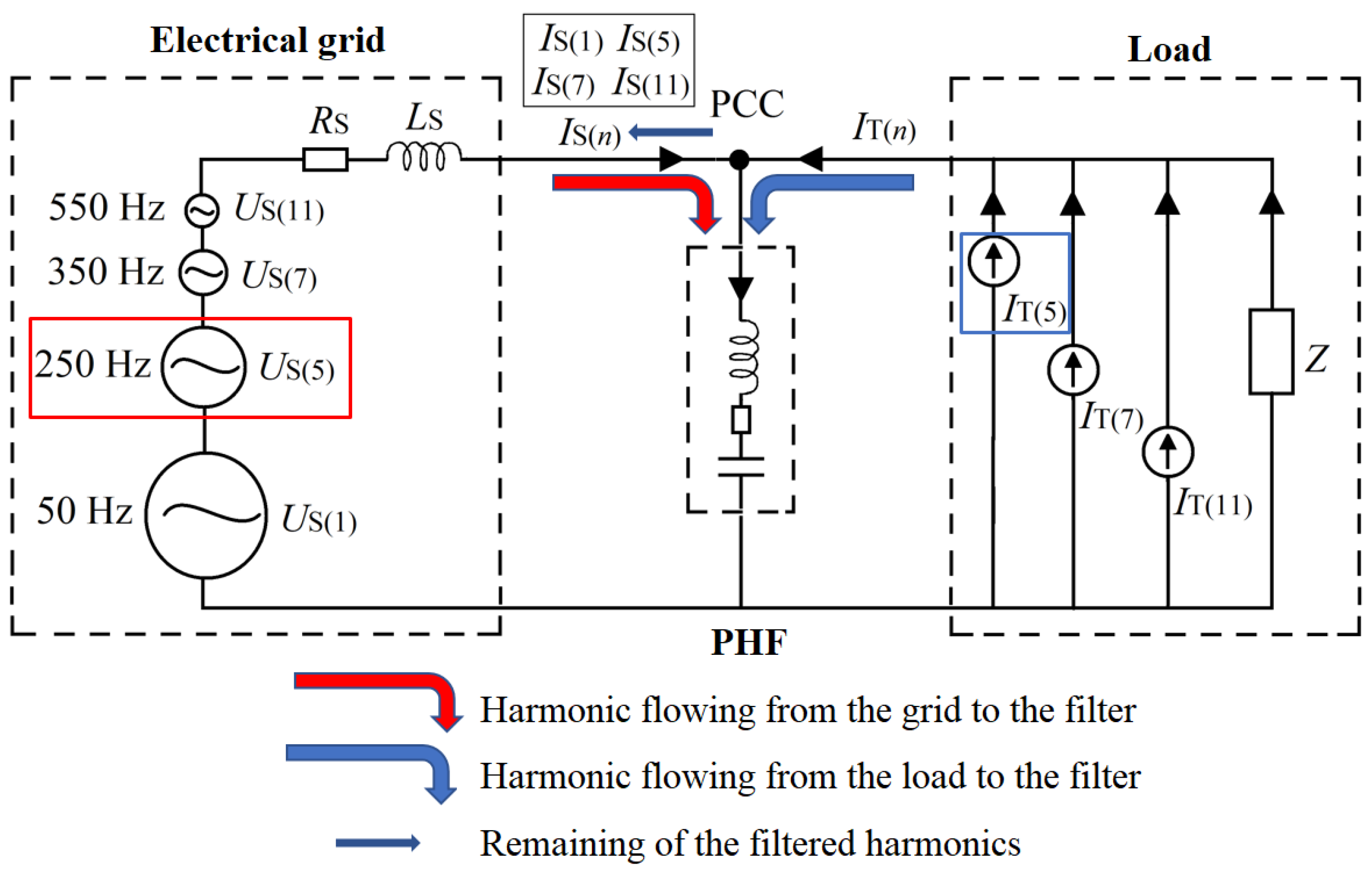
With the distorted waveform of the supply voltage, the grid behaves as a source of currents harmonics which may flow from the grid to the filter, especially the current of harmonic to be eliminated, which is at the grid side, because the filter, being tuned to that harmonic, has a small impedance for it.
-
The PHF resonance frequency should be chosen below the frequency of harmonic to be eliminated, taking into account the grid equivalent impedance of that harmonic. The filter equivalent impedance of the harmonic to be eliminated should be smaller than the grid equivalent impedance of that harmonic.
-
Because of the manufacturer tolerance, the filter elements (reactor and capacitor) should be well investigated in the laboratory after their obtaining from the producer to know their real parameters.
These investigations have also shown that the harmonics contained in the electrical grid flows through the filter, mostly those with frequencies close to the filter resonance frequency. The filtering efficiency depends upon the electrical grid impedance and that dependency can be reduced by adding the line reactor between the filter and the PCC. The line reactor presence does not only mitigate the amplitude of the current harmonics flowing from the electrical grid, but it also increases the grid voltage distortion.
The most important steps of designing the PHFs are: the investigations on the load current and voltage characteristic harmonics and fundamental harmonic reactive power; the electrical grid short-circuit power estimation; the analysis of the supply voltage spectrum at the PCC (before any load connection); the filter parameter computation. These steps have been detailed in this paper.
In Figure 65 and Figure 66, summary comparison graphs showing how an additional line reactor can be used to mitigate the harmonics amplification (e.g., the 5th) occurring between the filter (PCC) and the grid are presented.
In the summary comparison graphs in Figure 67, it is presented the behavior of the 5th harmonic in the voltage spectrums as well as in the current spectrums during the filter detuning phenomena. In the case of the Chroma supply voltage with harmonics, the amplitude of the 5th harmonic in the voltage spectrum is not reduced in the same way as in the current spectrum. The same situation can also be observed in the case of the electrical gird.
The last part of the paper concerns the investigation of PHFs in the electrical system with more complex loads. In the domain of harmonics filtration, this paper is expected to bring many recommendations.

Author Contributions

Conceptualization, C.S.A.M. and Z.H.; methodology, C.S.A.M.; software, C.S.A.M.; validation, Z.H.; formal analysis, C.S.A.M.; investigation, C.S.A.M.; resources, C.S.A.M.; data curation, C.S.A.M.; writing—original draft preparation, C.S.A.M.; writing—review and editing, Z.H.; visualization, Z.H.; supervision, Z.H.; project administration, A.F.; funding acquisition, (no funding). All authors have read and agreed to the published version of the manuscript.

Funding

This research received no external funding.

Institutional Review Board Statement

Not applicable.

Informed Consent Statement

Not applicable.

Data Availability Statement

Not applicable.

Conflicts of Interest

The authors declare no conflict of interest.

Appendix A

Figure A1. Three-phase capacitor bank and reactors (filter elements).
Energies 15 01894 g0a1
Figure A2. (a) Equivalent circuit in which the filter capacitors and reactors parameters were verified, (b) model in the laboratory.
Energies 15 01894 g0a2
R Lf = P I 2 L f = ( U I ) 2 R L f 2 ω ( 1 )
R C 1 = P I 2 C 1 = 1 ω ( 1 ) ( U I ) 2 R C 1 2 C f Δ = 2 3   C 1

References

  1. Azebaze, M.C.S.; Firlit, A. Investigation of the line-reactor influence on the active power filter and hybrid active power filter efficiency: Practical approach. Przegląd Elektrotechniczny 2021, 97, 39–44. [Google Scholar]
  2. Juan, W.D.; Contardo, J.M.; Moran, L.A. A Fuzzy-controlled active front-end rectifier with current harmonic filtering characteristics and minimum sensing variables. IEEE Trans. Power Electron. 1999, 14, 724–729. [Google Scholar] [CrossRef]
  3. Kwak, S.; Toliyat, H.A. Design and rating comparison of PWM voltage source rectifiers and active power filters for AC drives with unity power factor. IEEE Trans. Power Electron. 2005, 20, 1133–1142. [Google Scholar] [CrossRef]
  4. Firlit, A.; Kołek, K.; Piątek, K. Heterogeneous active power filter controller. In Proceedings of the IEEE International Symposium ELMAR, Zadar, Croatia, 18–20 September 2017. [Google Scholar]
  5. Ehsan, P.; Masood, A.A. Efficient procedures to design and characterize passive harmonic filters in low power applications. In Proceedings of the IEEE International Symposium on Industrial Electronics (ISIE), Bari, Italy, 4–7 July 2010. [Google Scholar]
  6. Park, B.; Lee, J.; Yoo, H.; Jang, G. Harmonic mitigation using passive harmonic filters: Case study in a steel mill power system. Energies 2021, 14, 2278. [Google Scholar] [CrossRef]
  7. Reynaldo, R.; Gregory, A.F. Optimal harmonic filter topology applied in HV and EHV networks using particle swarm optimization. In Proceedings of the IEEE Electrical Power and Energy Conference (EPEC), Ottawa, ON, Canada, 12–14 October 2016. [Google Scholar]
  8. Arrillaga, J.; Bradley, D.A.; Bodger, P.S. Power System Harmonics; John Wiley & Sons: Chichester, UK, 1985. [Google Scholar]
  9. Yousif, S.N.A.L.; Wanik, M.Z.C. Implementation of different passive filter designs for harmonic mitigation. In Proceedings of the IEEE Conference on National Power and Energy, PECon, Kuala Lumpur, Malaysia, 29–30 November 2004. [Google Scholar]
  10. Wu, C.-J.; Chiang, J.-C.; Liao, C.-J.; Yen, S.-S.; Yang, J.-S.; Guo, T.-Y. Investigation and mitigation of harmonic amplification problems caused by single-tuned filter. IEEE Trans. Power Deliv. 1998, 13, 800–806. [Google Scholar]
  11. Faraby, M.D.; Fitriati, A.; Muchtar, A.; Putri, A.N. Single tuned filter planning to mitigate harmonic polluted in radial distribution network using particle swarm optimization. In Proceedings of the IEEE 3rd International Seminar on Research of Information Technology and Intelligent Systems (ISRITI), Yogyakarta, Indonesia, 10–11 December 2020. [Google Scholar]
  12. Setiabudy, R.; Wibowo, G.P.; Herlina. Selection of single-tuned filter and high pass damped filter with changes of inverter type to reduce harmonics on microgrid AC-DC. In Proceedings of the IEEE International Conference on Electrical Engineering and Computer Science (ICECOS), Pangkal, Indonesia, 2–4 October 2018. [Google Scholar]
  13. Abdul, K.N.H.B.; Zobaa, A.F. Optimal single tuned damped filter for mitigating harmonics using MIDACO. In Proceedings of the IEEE International Conference on Environment and Electrical Engineering and IEEE Industrial and Commercial Power Systems Europe (EEEIC/I&CPS Europe), Milan, Italy, 6–9 June 2017. [Google Scholar]
  14. Abbas, A.S.; Ali, E.S.; El-Sehiemy, R.A.; Abou El-Ela, A.A.; Fetyan, K.M. Comprehensive parametric analysis of single tuned filter in distribution systems. In Proceedings of the IEEE 21st International Middle East Power Systems Conference (MEPCON), Cairo, Egypt, 17–19 December 2019. [Google Scholar]
  15. Muhammad, R.; Muhammad, I.; Danang, S. Single tuned harmonic filter as total harmonic distortion (THD) compensator. In Proceedings of the CIRED, 23rd International Conference on Electricity Distribution, Lyon, France, 15–18 June 2015; p. 0056. [Google Scholar]
  16. Sakar, S.; Karaoglan, A.D.; Balci, M.E.; Abdel Aleem, S.H.E.; Zobaa, A.F. Optimal design of single-tuned passive filter using response surface methodology. In Proceedings of the IEEE International Conference, ISNCC, Łagow, Poland, 15–18 June 2015. [Google Scholar]
  17. Klempka, R. Optimal Double-Tuned Filter Efficiency analysis. IEEE Trans. Power Deliv. 2020, 36, 1079–1088. [Google Scholar] [CrossRef]
  18. Azebaze, M.C.S.; Hanzelka, Z. LC Passive Harmonic Filters-Comparative Analysis between the Double-Tuned Filter and Two Single-Tuned Filter. In Polish-Filtry Pasywne LC-Analiza Porównawcza Filtru Podwójnie Nastrojonego I Dwóch Filtrów Jednogałęziowych; Grupa MEDIUM Sp. z o.o. Sp.k.-a: Cracow, Poland, 2021; pp. 50–54. [Google Scholar]
  19. Min-cia, K.; Xinzhou, D. The parameters calculation and simulation research of two-type double-tuned Filter. In Proceedings of the IEEE Transmission and Distribution Conference and Exposition, Asia and Pacific, Seoul, Korea, 26–30 October 2009. [Google Scholar]
  20. Haposan, Y.P.N.; Chairul, G.I. A new algorithm for designing the parameter of the damped-type double tune filter. In Proceedings of the IEEE 5th International Conference on Electrical Engineering, Computer Science and Informatics (EECSI), Malang, Indonesia, 16–18 October 2018. [Google Scholar]
  21. Ahmed, M.; Al Nahid-Al-Masood, N.; Huq, S.I.; Khan, F.I.; Juberi, H.; Bashar, S. A comprehensive modeling of double tuned filter for efficient mitigation of harmonic distortion. In Proceedings of the IEEE International Conference on Smart Grids and Energy Systems (SGES), Perth, Australia, 23–26 November 2020. [Google Scholar]
  22. Zobaa, A.; Ahady, H.E.A.A.; Hosam, K.M.Y. Comparative analysis of double-tuned harmonic passive filter design methodologies using slime mould optimization algorithm. In Proceedings of the IEEE Texas Power and Energy Conference (TPEC), College Station, TX, USA, 2–5 February 2021. [Google Scholar]
  23. Kang, M.-C.; Zhou, J.-H. Compensates the double tuned filter element parameter change based on the controllable reactor. In Proceedings of the IEEE International Conference on Electricity Distribution, CICED, Guangzhou, China, 10–13 December 2008. [Google Scholar]
  24. Mingcai, K.; Zhiqian, B.; Xiping, Z. The parameters calculation and simulation research about two types structure of double-tuned Filter. In Proceedings of the IEEE 45th International Conference on Universities Power Engineering, Cardiff, UK, 31 August–3 September 2010. [Google Scholar]
  25. Klempka, R. Passive power filter design using genetic algorithm. Przegląd Elektrotechniczny 2013, 5, 89. [Google Scholar]
  26. Yi-Hong, H.E.; Heng, S.U. A new method of designing double-tuned filter. In Proceedings of the International Conference on Computer Science and Electronics Engineering, Hangzhou, China, 22–23 March 2013. [Google Scholar]
  27. Mingtao, Y.; Jianye, C.; Weian, W.; Zanji, W. A double tuned filter based on controllable reactor, IEEE International Symposium on Power Electronics. In Proceedings of the Electrical Drives, Automation and Motion, SPEEDAM, Taormina, Italy, 23–26 May 2006. [Google Scholar]
  28. Xiao, Y. Algorithm for the parameters of double tuned filter. In Proceedings of the IEEE 8th International conference on Harmonics and Quality of Power Proceedings, Athens, Greece, 14–16 October 1998. [Google Scholar]
  29. Bartzsch, C.; Huang, H.; Roessel, R.; Sadek, K. Triple tuned harmonic filters-Design principle and operating experience. In Proceedings of the International Conference on Power System Technology, Kunming, China, 13–17 October 2002. [Google Scholar]
  30. Chen, B.; Zeng, X.; Xv, Y. Three tuned passive filter to improve power quality. In Proceedings of the IEEE International Conference on Power System Technology, PowerCon, Chongqing, China, 22–26 October 2006. [Google Scholar]
  31. Bhim, S.; Ambrish, C.; Kamal, A.-H. Power Quality: Problems and Mitigation Techniques; John Wiley & Sons Ltd., The Atrium, Southern Gate: Chichester, UK, 2015. [Google Scholar]
  32. Azebaze, M.C.S.; Hanzelka, Z. Passive Harmonic Filters. In Power Quality in Future Electrical Power Systems, 1st ed.; Zobaa, A.F., Shady, H.E.A.A., Eds.; IET the Institution of Engineering and Technology: London, UK, 2017; pp. 77–127. [Google Scholar]
  33. Bhim, S.; Vishal, V.; Vipin, G. Passive hybrid filter for varying rectifier loads. In Proceedings of the IEEE International Conference on Power Electronics and Drives Systems, PEDS, Kuala Lumpur, Malaysia, 28 November–1 December 2005. [Google Scholar]
  34. Azebaze, M.C.S.; Hanzelka, Z. Application of C-type filter to DC adjustable speed drive. In Proceedings of the IEEE International Conference-Modern Electric Power Systems, Poland, Wroclaw, 6–9 July 2015; pp. 1–7. [Google Scholar]
  35. Klempka, R. Design of C-type passive filter for arc furnaces. Metalurgia 2017, 56, 161–163. [Google Scholar]
  36. Xiao, Y. The method for designing the third order filter. In Proceedings of the IEEE International Conference on Harmonics and Quality of Power Proceedings, Wuhan, China, 14–16 October 1998. [Google Scholar]
  37. Tianyu, D. Design Method for Third-Order High-Pass Filter. IEEE Trans. Power Deliv. 2016, 31, 402–403. [Google Scholar]
  38. Hanzelka, Z. The Process of Connecting the Capacitor Banks; In Polish-Proces Łączenia Baterii Kondensatorów. pp. 1–27. Available online: http://www.twelvee.com.pl/42767005.php?c=%D0%B5 (accessed on 20 February 2021).
  39. Klempka, R. A New Method for the C-Type Passive Filter Design. J. Przegląd Elektrotechniczny 2012, 88, 277–281. [Google Scholar]
  40. James, K.P. A transfer function approach to harmonic filter design. IEEE Ind. Appl. Mag. 1997, 3, 68–82. [Google Scholar]
  41. Jinhao, W.; Tingdong, Z. Passive filter design with considering characteristic harmonics and harmonic resonance of electrified railway. In Proceedings of the IEEE 8th International Conference on Mechanical and Intelligent Manufacturing Technologies (ICMIMT), Cape Town, South Africa, 3–6 February 2017. [Google Scholar]
  42. Klempka, R. An arc furnace as a source of voltage disturbances-A statistical evaluation of propagation in the supply network. Energies 2021, 14, 1076. [Google Scholar] [CrossRef]
  43. Azebaze, M.C.S.; Hanzelka, Z. Different approaches for designing the passive power filters. Przegląd Elektrotechniczny 2015, 91, 102–108. [Google Scholar]
  44. Klempka, R. Design and Optimization of a Simple Filter Group for Reactive Power Distribution; Hindawi Publishing Corporation: London, UK, 2016. [Google Scholar]
  45. Junpeng, J.; Zeng, G.; Liu, H.; Luo, L.; Zhang, J. Research on selection method of passive power filter topologies. In Proceedings of the IEEE International Conference on Power Electronics and Motion Control, Harbin, China, 2–5 June 2012. [Google Scholar]
  46. Klempka, R. Designing a group of single-branch filters taking into account their mutual influence. Arch. Electr. Eng. 2014, 63, 81–91. [Google Scholar] [CrossRef]
  47. Jandecy, C.L.; Ignacio, P.A.; Maria Emilia de, L.T.; de Oliveira, R.C.L. Multi-objective optimization of passive filters in industrial power systems. Electr. Eng. Mar. 2017, 99, 387–395. [Google Scholar]
  48. Klempka, R. Analytical optimization of the filtration effiency of a group of single branch filtres. ELSEVIER. Electr. Power Syst. Res. 2022, 202, 107603. [Google Scholar] [CrossRef]
  49. Klempka, R. Designing a group of single-branch filters. In Proceedings of the 7th International Conference on Electrical Power Quality and Utilisation, Cracow, Poland, 17–19 September 2003. [Google Scholar]
  50. Tazky, M.; Regula, M.; Otcenasova, A. Impact of changes in a distribution network nature on the capacitive reactive power flow into the transmission network in Slovakia. Energies 2021, 14, 5321. [Google Scholar] [CrossRef]
  51. AbdElhafez, A.A.; Alruways, S.H.; Alsaif, Y.A.; Althobaiti, M.F.; Alotaibi, A.B.; Alotaibi, N.A. Reactive power problem and solutions: An overview. J. Power Energy Eng. 2017, 5, 40–54. [Google Scholar] [CrossRef] [Green Version]
  52. Shawon, M.H.; Hanzelka, Z.; Dziadecki, A. Voltage-current and harmonic characteristic analysis of different FC-TCR based SVC. In Proceedings of the IEEE Conference Eindhoven PowerTech, Eindhoven, The Netherlands, 29 June–2 July 2015. [Google Scholar]
  53. Hanzelka, Z. The Higher Harmonics fo the Voltage and Current; In Polish-Wyższy Harmoniczne Napięć i Prądów. pp. 1–30. Available online: http://www.twelvee.com.pl/42767005.php?c=%D0%B5 (accessed on 20 February 2021).
  54. Harmonics in Power System-Siemens Industry, Inc. 2013. Available online: https://assets.new.siemens.com/siemens/assets/api/uuid:8ab2a02e-ad94-41cb-a362-438f016aa704/drive-harmonics-in-power-systems-whitepaper.pdf (accessed on 2 March 2021).
  55. Harmonic Mitigation for AC Variable Frequency Pump Drives, World PUMPS, December 2002. Available online: http://www.mirusinternational.com/downloads/World%20Pumps%20-%20Harmonic%20Mitigation%20for%20AC%20Variable%20Frequency%20Pump%20Drives.pdf (accessed on 2 March 2021).
  56. Kuldeep, K.S.; Saquib, S.; Nanand, V.P. Harmonics & its mitigation technique by passive shunt filter. Int. J. Soft Comput. Eng. (IJSCE) 2013, 3, 325–331. [Google Scholar]
  57. Singh, G.K. Power System Harmonic Research: A Survey. Wiley InterScience Eur. Trans. Electr. Power 2009, 19, 151–172. [Google Scholar] [CrossRef]
  58. Wagner, V.E. Effects of harmonics on equipment. IEEE Trans. Power Deliv. 1993, 8, 672–680. [Google Scholar] [CrossRef]
  59. Azebaze, M.C.S. Investigation on the work efficiency of the LC passive harmonic filter chosen topologies. Electronics 2021, 10, 896. [Google Scholar] [CrossRef]
  60. Mtakati, M.; Freere, P.; Roberts, A. Design and comparison of four branch passive harmonic filters in three phase four Wire systems. In Proceedings of the IEEE AFRICON Conferences, Accra, Ghana, 25–27 September 2019. [Google Scholar]
  61. Abu-Rubu, H.; Iqbal, A.; Guzinski, J. High Performance Control of AC Drives with MATLAB/SIMULINK Models; John Wiley & Sons: Chichester, UK, 2012. [Google Scholar]
  62. Available online: https://www.a-eberle.de/en/product-groups/pq-mobile/devices/pq-box-200 (accessed on 2 March 2021).
  63. Hanzelka, Z. Quality of the Electricity Supply-Disturbances of the Voltage RMS Value. In Polish–Jakość Dostawy Energii Elektrycznej-Zaburzenia Wartości Skutecznej Napięcia; AGH: Cracow, Poland, 2013. [Google Scholar]
  64. Muhammad, H.R. Power Electronics Handbook; Elsevier: San Diego, CA, USA, 2011; Available online: http://site.iugaza.edu.ps/malramlawi/files/RASHID_Power_Electronics_Handbook.pdf (accessed on 2 March 2021).
  65. Visintini, R. Rectifiers, Elettra Synchrotron Light Laboratory, Trieste, Italy. Available online: https://cds.cern.ch/record/987551/files/p133.pdf (accessed on 2 March 2021).
  66. Available online: http://www.chromaate.com (accessed on 2 March 2021).
  67. Das, J.C. Passive filters-potentialities and limitations. IEEE Trans. Ind. Appl. 2004, 40, 232–241. [Google Scholar] [CrossRef]
  68. Young-Sik, C.; Hanju, C. Single-tuned passive harmonic filter design considering variances of tuning and quality factor. J. Int. Counc. Electr. Eng. 2011, 1, 7–13. [Google Scholar]
Figure 1. Block diagram representing the laboratory setup. Iref—external reference current.
Energies 15 01894 g001
Figure 2. (a) Parameters of the electrical grid supplying the laboratory setup, (b) electrical grid equivalent circuit. Sec—Secondary, Pri—primary.
Energies 15 01894 g002
Figure 3. PCC voltage waveforms (a) and its spectrum (p.u.) (b) when the considered load is not connected (measured).
Energies 15 01894 g003
Figure 4. Voltage and current at the rectifier DC side for different firing angle values: (a) continuous mode (θ = 30°); (b) discontinuous mode (θ = 60°) (from simulation).
Energies 15 01894 g004
Figure 5. Examples of the measured PCC phase voltage and current for different values of DC voltage and firing angle: (a) UDC = 20 V; (b) UDC = 70 V; (c) UDC = 360 V; (d) UDC = 525 V.
Energies 15 01894 g005
Figure 6. Grid voltage and current parameters measured from the laboratory setup. The example of waveforms is for the UDC equal to 250 V.
Energies 15 01894 g006
Figure 7. Example of the measured grid current spectrum for UDC = 250 V (the red manganese color represents the characteristic harmonics).
Energies 15 01894 g007
Figure 8. Comparison between laboratory and simulated characteristics: (a,b) PCC voltage and current fundamental harmonic vs. rectifier firing angle; (c,d) PCC voltage and current fundamental harmonic vs. rectifier DC voltage.
Energies 15 01894 g008
Figure 9. Comparison between the laboratory and simulated characteristics: PCC voltage and current 5th harmonic versus rectifier firing angle (a,b) and versus rectifier DC voltage (c,d).
Energies 15 01894 g009
Figure 10. Comparison between the laboratory and simulated characteristics: PCC voltage and current 7th harmonic versus rectifier firing angle (a,b) and versus rectifier DC voltage (c,d).
Energies 15 01894 g010
Figure 11. Fundamental harmonic PCC active and reactive powers versus firing angle and versus UDC (one-phase): (a) laboratory data; (b) simulated data.
Energies 15 01894 g011
Figure 12. (a) Single-tuned filter, (b) expressions used to compute the single-tuned filter parameters. ωre—resonance frequency, nre—harmonic order at the resonance, qLf—reactor quality factor, ω(1) = 2π f(1).
Energies 15 01894 g012
Figure 13. Filter impedance versus frequency characteristic (simulation).
Energies 15 01894 g013
Figure 14. Equivalent electrical circuit used to measure the single-tuned filter impedance versus frequency characteristics (Chroma [66]).
Energies 15 01894 g014
Figure 15. Single-tuned filter impedance versus frequency characteristic measured in the laboratory.
Energies 15 01894 g015
Figure 16. Equivalent circuit of the laboratory model with 5th harmonic single-tuned filter together with the measured parameters.
Energies 15 01894 g016
Figure 17. Grid voltage (US1) and current (IS1) waveforms with their spectrums (after the filter connection).
Energies 15 01894 g017
Figure 18. Input rectifier (IT1) current with its spectrum and filter current (If1) with the spectrum.
Energies 15 01894 g018
Figure 19. (a) Grid voltage THD; grid voltage 5th (b) and 7th (c) harmonic amplitudes before and after the filter connection.
Energies 15 01894 g019
Figure 20. (a) Single-tuned filter work efficiency, (b) the 5th harmonic current amplitude generated by the load (IT(5)) is compared to the 5th harmonic current amplitude at the grid side (IS(5)) for different firing angle.
Energies 15 01894 g020
Figure 21. Experiments with the programmable voltage source Chroma: equivalent circuit of the laboratory model.
Energies 15 01894 g021
Figure 22. Voltage waveforms and spectrum measured at the programmable AC voltage source terminals when no load and filter were connected: (a) voltage with harmonics; (b) voltage without harmonics.
Energies 15 01894 g022
Figure 23. Waveforms and spectrums when the filter is not connected: (a) PCC voltage waveform with (b) its spectrum, (c) voltage source input current with (d) its spectrum (only the load is connected).
Energies 15 01894 g023
Figure 24. Waveforms and spectrums when the filter is not connected: (a) PCC voltage waveform with (b) its spectrum, (c) voltage source input current with (d) its spectrum (only the load is connected).
Energies 15 01894 g024
Figure 25. (a) PCC voltage waveform with (b) its spectrum, (c) voltage source input current with (d) its spectrum (load and filter connected).
Energies 15 01894 g025
Figure 26. (a) PCC voltage waveform with the spectrum (b), (c) voltage source input current with the spectrum (d) (load and filter connected).
Energies 15 01894 g026
Figure 27. (a) Rectifier input current waveform with (b) its spectrum, (c) filter current waveform with (d) its spectrum.
Energies 15 01894 g027
Figure 28. (a) Rectifier input current waveform with (b) its spectrum, (c) filter current waveform with (d) its spectrum.
Energies 15 01894 g028
Figure 29. Comparison between the spectrums of filter efficiency: (a) programmable voltage source with harmonic, (b) programmable voltage source without harmonics.
Energies 15 01894 g029
Figure 30. (a,b) The amplitude of the 5th harmonic current measured at the load input (IT1(5)) is compared to the one measured at the Chroma voltage source input (IS1(5)); (c,d) the THD of the load input current (THDIT1) is compared to the one of the Chroma input currents (THDIS1).
Energies 15 01894 g030
Figure 31. Experiments with the programmable voltage source: equivalent circuit of the laboratory model with the additional line-reactor LSS. The line reactor parameters were measured in the laboratory.
Energies 15 01894 g031
Figure 32. PCC voltage waveforms and spectrums measured at the PCC when the programmable voltage source was: (a) with harmonics and (b) without harmonics. The line reactor LSS is considered.
Energies 15 01894 g032
Figure 33. Current waveforms and spectrums measured at the input of the Chroma voltage source with (a) harmonics and (b) without harmonics. The line reactor LSS is considered.
Energies 15 01894 g033
Figure 34. Current waveforms and spectrums measured at the filter terminals when the programmable voltage source was with: (a) harmonics and (b) without harmonics. The line reactor LSS is considered.
Energies 15 01894 g034
Figure 35. Current waveforms and spectrums measured at the load terminals when the programmable voltage source was with: (a) harmonics and (b) without harmonics. The line reactor LSS is considered.
Energies 15 01894 g035
Figure 36. Filter efficiency when the programmable voltage source was with: (a) harmonics and (b) without harmonics. The line reactor LSS is considered.
Energies 15 01894 g036
Figure 37. The amplitude (a,b) of the 5th harmonic current, as well as the current THD (c,d) measured at the load input, are compared to the ones measured at the Chroma voltage source input. The line reactor LSS is considered.
Energies 15 01894 g037
Figure 38. Comparison between the filter power losses (the fundamental harmonic) when the additional line reactor LSS is connected and when it is not connected: Chroma voltage source with (a) and without (b) harmonics.
Energies 15 01894 g038
Figure 39. Equivalent circuit of laboratory model with line reactor.
Energies 15 01894 g039
Figure 40. Grid voltage and current waveforms together with the spectrums (with LSS).
Energies 15 01894 g040
Figure 41. Comparison before and after the line reactor connection of the PCC voltage THD (a) and grid current THD (b).
Energies 15 01894 g041
Figure 42. Comparison between the PCC voltage (a) and current (b) fundamental harmonic before and after the line reactor connection.
Energies 15 01894 g042
Figure 43. Voltage waveforms measured at different points of laboratory model. The influence of the reactor inductance on the depth of the commutation notches is presented (measured).
Energies 15 01894 g043
Figure 44. Laboratory setup with the single-tuned filter after the line reactor connection.
Energies 15 01894 g044
Figure 45. Laboratory equivalent circuit with filter and line reactor.
Energies 15 01894 g045
Figure 46. Waveforms and spectrums of grid current and voltage.
Energies 15 01894 g046
Figure 47. Waveforms and spectrums of input rectifier current (IT1) and filter current (If1).
Energies 15 01894 g047
Figure 48. (a) Filter electiveness, (b) comparison between the 5th harmonic current of grid (IS(5)) and the input rectifier (IT(5)).
Energies 15 01894 g048
Figure 49. Grid voltage and current spectrum: the case without the filter is compared to the case with filter (UDC equal to 250 V).
Energies 15 01894 g049
Figure 50. THD of grid voltage (a) and current (b) for different UDC: the case without the filter is compared to the case with filter.
Energies 15 01894 g050
Figure 51. Impedance versus frequency characteristic observed at the load input (from the simulated model).
Energies 15 01894 g051
Figure 52. Power system equivalent circuit with filter reactor parameters.
Energies 15 01894 g052
Figure 53. Filter impedance versus frequency characteristics: (a) expected characteristics from simulation and (b) characteristics measured in the laboratory.
Energies 15 01894 g053
Figure 54. Point of common coupling voltage and current waveforms and spectrums.
Energies 15 01894 g054
Figure 55. Input rectifier and filter current waveforms and spectrums.
Energies 15 01894 g055
Figure 56. THD of the grid voltage (a) and current (b) for different resonance frequencies.
Energies 15 01894 g056
Figure 57. The 5th harmonic reduction efficiency.
Energies 15 01894 g057
Figure 58. (a) PCC voltage waveform with (b) its spectrum, (c) Chroma input current with (d) its spectrum.
Energies 15 01894 g058
Figure 59. (a) PCC voltage waveform with the spectrum (b), (c) Chroma input current with the spectrum (d).
Energies 15 01894 g059
Figure 60. (a) Rectifier input current waveform with (b) the spectrum, (c) filter current waveform with (d) the spectrum.
Energies 15 01894 g060
Figure 61. (a) Rectifier input current waveform with (b) the spectrum, (c) filter current waveform with (d) the spectrum.
Energies 15 01894 g061
Figure 62. PCC voltage (a) and current (b) THD.
Energies 15 01894 g062
Figure 63. PCC voltage (a) and current (b) THD.
Energies 15 01894 g063
Figure 64. Equivalent circuit of the electrical system showing the flow of harmonics.
Energies 15 01894 g064
Figure 65. Summary comparison graph of the experiments performed after connecting the filter at the PCC between the programmable voltage source and the load: (a,c) filter efficiency and (b,d) the amplitude of the 5th harmonic current at the Chroma input (IS(5)) is compared to the one at load input (IT(5)). In (a,c), the amplitudes above 100% mean harmonic amplification at the Chroma input. The graphs are well described in the text.
Energies 15 01894 g065
Figure 66. Summary comparison graph of the experiments performed after connecting the filter at the PCC between the grid and the load: (a,c) filter efficiency and (b,d) the amplitude of the 5th harmonic current at the grid side (IS(5)) is compared to the one at load side (IT(5)). The graphs are well described in the text.
Energies 15 01894 g066
Figure 67. Summary comparison graphs presenting the behavior of the 5th harmonic in the voltage spectrums (a,b,e) as well as in the current spectrums (c,d,f) during the filter detuning phenomena. In the case of the supply voltage without harmonics (Chroma), the amplitude of the 5th harmonic in the voltage spectrum is reduced in the same way as in the current spectrum. The graphs are well described in the text.
Energies 15 01894 g067
Table 1. Computed equivalent parameters of the single-tuned filter (one-phase).
nreQf
[Var]
Uf
[V]
Lf
[mH]
Cfy
[µF]
C
[µF]
Zf(1)
[Ω]
Zf(5)
[Ω]
4.910002307.357.619.2530.45
Table 2. Technical data of the filter reactors and capacitor (from manufacturer).
Core ReactorsThree-Phase Gas Insulated Power Capacitor
Inductance8.03; 7.7; 7.3; 7.0; 6.6 [mH]Voltage 400 [V]
Current15 [A]Power2.9 [kVar]
Frequency50 [Hz]Rated current4.18 [A]
Nominal Voltage 400 [V]Capacitance (Cf∆)19.2 [µF]
Inductance Tolerance± 10%Capacitance tolerance−5…+10%
Mass≈12 [kg]Ambient temperature−25…+50 °C
Power0.57 kVarDischarge50V/1 min
Winding materialCopperFrequency50 [Hz]
Table 3. The parameters of the filter elements from the manufacturer are compared to those measured in the laboratory.
Reactor
Parameters from ManufacturerMeasured Parameters in the Laboratory
L [mH]U [V]I [A]P [W]RLf [Ω]Lf [mH]ZLf(1) [Ω]
8.0313.1957.50.38.342.638
7.712.6757.50.38.002.534
7.312.1757.50.37.682.434
711.6557.50.37.352.33
6.611.0857.50.36.982.216
Capacitor bank
C1 [µF]U [V]I [A]P [W]RC1 [Ω]Cf∆ [µF]
19.22412.20019.4
Table 4. Single-tuned filters resonance frequencies: the frequencies obtained from manufacturer data are compared to the frequencies obtained from the data in Table 3 and to the measured frequencies from the electrical circuit of Figure 14.
Frequencies from ManufacturerComputed Frequencies
(from Table 3)
Measured Frequencies
in the Laboratory (From Figure 16)
nrefre [Hz]nrefre [Hz]nrefre [Hz]
4.682344.57228.54.57228.5
4.782394.662334.67233.5
4.92454.762384.77238.5
5.012250.64.862434.89244.5
5.162584.99249.55.04252
Table 5. Summarized single-tuned filter parameters (one phase).
nreQf [Var]Uf [V]RLf [Ω]Lf [mH]qLfCfy [µF]C [µF]Zf(1) [Ω]Zf(5) [Ω]
Theoretical Computed Parameters
4.9100023007.357.619.2530.45
Manufacturer parameters
4.9966.66230-7.3-57.619.2530.45
Measured parameters in the laboratory
4.77966.662300.37.688.0458.219.452.281.16
Table 6. Power system parameters measured in the laboratory for different rectifier firing angles (after the filter connection). DPF–displacement power factor; QS1(1), Qf1(1), and QT1(1) are, respectively, the grid, filter, and load fundamental reactive powers. PS1(1) and Pf1(1) are, respectively, the grid and filter active powers.
UDC
[V]
θ
[deg.]
THDUS1 [%]THDIS1 [%]THDIT1 [%]DPFPS1(1)
[W]
Pf1(1)
[W]
QS1(1)
[Var]
Qf1(1)
[Var]
QT1(1)
[Var]
5095.232.06100.3257.370.0752.5212.56−757.17−993.82243.05
15076.312.12156.0964.400.84381.7213.82−242.01−987.57749.65
25026.542.2065.4660.620.99824.4017.3861.79−983.801048.1
35033.572.2451.3343.630.981396.319.39233.94−989.891225.4
45033.572.0655.6235.140.992105.722.1549.58−989.381040.3
52513.541.8136.5729.240.942680.224.60−883.24−975.2195.52
Table 7. Parameters of the fundamental harmonic active and reactive powers as well as DPF for different rectifier firing angles measured at the PCC.
UDC [V]θ [deg.]PS1(1) [W]QS1(1) [Var]DPF
5095.2373.13269.020.26
15076.31387.71743.750.46
25026.54805.2610790.59
35033.571371.81214.30.74
45033.572091.1995.880.90
52513.542605.4340.860.99
Table 8. Power system parameters measured in the laboratory for different rectifier firing angles.
UDC
[V]
θ
[deg.]
THDUS1 [%]THDIS1 [%]THDIT1 [%]DPFPS1(1)
[W]
QS1(1)
[Var]
Pf1(1)
[W]
Qf1(1)
[Var]
QT1(1)
[Var]
5095.234.56 38.47 131.950.0863.80−743.2713.31−1022.6283.91
15076.316.7277.4685.330.82394.58−267.7316.28−1003.9738.73
25026.548.1938.7958.510.99818.2984.5417.53−992.401078.0
35033.578.5225.3943.780.981370244.6118.62−978.771223.5
45033.579.1019.7734.740.992082.256.7221.24−972.861029.9
52513.544.9512.1826.610.962668.1−750.0623.44−982.17235.02
Table 9. Fundamental harmonic active and reactive power measured in the laboratory model.
nrePS1(1) [W]QS1(1) [Var]Pf1(1) [W]Qf1(1) [Var]QT1(1) [Var]
No filter connected806.291065.6---
4.57821.6683.8116.99−981.841067.4
4.66826.1583.5316.10−991.201076.4
4.76815.8483.2116.90−971.231056.1
4.86807.3994.7316.10−943.331039.5
4.99819.6978.1117.46−965.521045.1
Publisher’s Note: MDPI stays neutral with regard to jurisdictional claims in published maps and institutional affiliations.

