1. Introduction
The coronavirus pandemic has turned the world upside down since the second quarter of 2020. The first sectors to be severely impacted by the coronavirus crisis were transport, tourism, and hospitality, as well as the event planning industry. There is no doubt that the tourism industry’s status quo has been severely impacted by the pandemic. The latest annual WTTC [
1] research shows that tourism suffered a loss of almost 5 trillion dollars in 2020, with the contribution to GDP falling by a staggering 49.1% compared with 2019. In 2020, 62 million jobs were lost, and domestic visitor spending fell by 45% [
2], while spending by international visitors fell by an unprecedented 69.4%.
There have been other crisis situations that have had a detrimental impact on tourism, including the financial crisis of 2008–2010, various international terrorism events [
3], including the fall of the twin towers in the United States of America in 2001, bankruptcies in tourism, and natural disasters, such as the 2021 volcanic eruption in Spain that disrupted a considerable number of European flights. However, these different crises did not have such a devastating impact on travel as the current pandemic, because they were not global events [
4]. In the case of COVID-19, once social distancing policies were implemented, there was a significant decrease in tourist arrivals, which reduced the total travel expense income at the point of destination. Tourism seems to be particularly vulnerable to health crises [
5], because policies apply [
6] to prevent the spread of contagions, such as restrictions on mobility and social distancing. These restrictions negatively affect most tourism-related services by impeding movement [
7] between regions or countries and changing travel motivations, which produces supply shocks [
8].
The forecasting of tourist activity in a pandemic is also hampered by the fact that tourism depends upon direct contact being established at the moment of consumption. Unlike the market for goods, in the purchase of a tourism product [
9], the consumer is faced with a series of uncertainties and much greater risks, which only arise during tourist consumption.
Any attempt to forecast tourism activity must consider two essential variables in tourist circulation, namely, seasonality and motivation. Tourist motivation includes needs, impulses, intentions, values, and specific tendencies, all of which have a personal feature. The motivation (vocation, inclination) generate tourist demand, which is always quite personal and subjective, and it is determined by psychological impulses [
10] and exogenous factors (environmental influences) [
11]. Thus, during the current pandemic, the uncertainty and risk to which a traveler is exposed causes their motivation to travel to decrease in intensity, which influences the dynamics of travel [
12]. The changes in tourism motivation are a balance between necessity and satisfaction, with the balance tipping in favor of the latter. On the one hand, satisfaction is one of the most important stimuli of international tourist traffic, whereas necessity tends to stimulate domestic tourist traffic. The basis for transforming tourist demand into consumption is mainly the motivation to travel. Tourist motivation is seen as a stimulating element of tourist traffic. There is an intrinsic link between motivation and tourist traffic, which is why in the absence of tourist motivation, any attempt to estimate passenger flows would be difficult to achieve and it would not be of practical applicability.
Given the current situation in Romania, which is still at the peak of the fourth wave of COVID-19 infections, we can say that in terms of both real risks and the emotional component, there will be a prolonged period in which we will see limited consumption of non-essential goods, a slowdown in activity in sectors where physical presence is required [
13], and a lower attractiveness of domestic and international travel and tourism packages.
One of the key differences of the tourism industry from other economic sectors is that, although health hazards do not destroy the infrastructure, they affect the flow [
9] of tourists. The emphasis of this paper is the ability and power to estimate tourist flow in the current, uncertain conditions.
For central authorities, but also for economic agents that are active in the field of tourism, the foreknowledge of a possible trend in the number of tourist arrivals is especially important for establishing a medium- to long-term strategy, depending on the risk and uncertainty of the conditions. Additionally, the possibility of estimating the flow of tourists is particularly useful for anticipating the necessary labor force in the field of tourism and HORECA, which are facing acute staff shortages in Romania. Estimating tourist arrivals allows for the hiring of immigrant workers as necessary.
The research presented in this paper has theoretical applicability, by establishing a forecast model of tourist flow in Romania in the context of the current pandemic, as well as in practice, through offering the possibility of anticipating tourist flow, according to which the Romanian decision-making bodies can establish the necessary measures to mitigate the negative effects of the pandemic upon Romanian tourism.
2. Literature Review
The literature review was approached in this study from two perspectives. On the one hand, some of the literature reflected the impact of the pandemic crisis caused by the SARS-CoV-2 virus on the entire tourism industry, and on the other hand, we reviewed the specialized literature on forecasting tourism.
2.1. The Impact of the COVID-19 Health Crisis on the Tourism Industry
The tourism sector is currently facing difficult times, as it is one of the most affected by the effects of the global pandemic [
14].
At the structural changes that are taking place at the social level and that affect [
15], among many other aspects, the way we work, consume and travel, there is a growing trend towards sustainability [
16,
17]—prior to the situation caused by COVID-19—which foreshadows that we are part of a fundamental transition in the vast majority of sectors [
18].
The HORECA sector, as a very important part of the tourism sector, is no stranger to this [
19], or to the need for a new management model that respects the environment and the limits of the planet, as it wishes to ensure the continuity of its activity [
20,
21].
The positive results obtained in 2019 have prepared the players in the field for a favorable evolution in 2020 [
22]. However, the traffic restrictions imposed during the state of emergency, some of which have been maintained and are on alert, have seriously affected the performance of this sector [
23].
Humanity is going through a period in which the pace of change [
24] is accelerating, with more and more aspects of the future being characterized by high levels of risk and uncertainty [
25]. As a result, the future no longer flows linearly from the past and the present; the discontinuities are multiplying [
26], which makes forecasting activity absolutely necessary [
27].
The actions are oriented towards excellence for the future [
28], which is why specialists from all over the world who undertake them are good and fine connoisseurs of forecasting methods [
29], procedures and techniques [
30].
Given the high degree of uncertainty that the future holds, the hypotheses acquire an increasingly important role in the forecasts of the tourism industry [
31].
Predictive studies in the field of tourism are all the more necessary [
32] as the share of tourism activities in all activities carried out at the level of a national economy become higher, the more the dynamics of changes in the field of tourism increases, the more ephemeral the market is and its fluctuations in demand, and the more unstable customers’ behavior becomes in the face of the global challenges posed by the COVID-19 pandemic [
33].
In general, there is a consensus on the importance of the forecasting and planning of activity in the tourism industry. Travel demand forecasting is essential in creating a rapid response to a variety of unexpected and unpredictable situations [
34] that arise in this activity in the current conditions of uncertainty [
35,
36].
Tourist flows in most destinations vary seasonally [
37]. Seasonality is one of the most important and distinctive features of tourism demand and has an important impact on the planning and operation of tourism business and on destination management [
38,
39] in terms of infrastructure and resource allocation [
40].
The tourist demand usually presents as seasonal models [
41]. One of the main characteristics of the tourist product is the existence of seasonal oscillations in the demand and implicitly of the production of the tourist services [
42]. These seasonal fluctuations are characterized by a high degree of tourist flows in certain periods of the calendar year and by a significant reduction in them or even a halt in tourist arrivals [
43].
Seasonality has direct consequences [
44] both on the development of tourism and on other branches of the national economy whose evolution is related to the development of tourism [
45]. The consequences of the seasonality of the tourist product demand [
46] determine either the incomplete use of the material base and the labor force with negative effects on the possibility of recovering the expenses (in the periods with reduced demand (pre-, post- and off-season), or of the accommodation, food and other categories of spaces that ensure the provision of tourist services as well as the service staff, which influence the quality of the services offered, and could cause dissatisfaction to tourists [
47].
Seasonal fluctuations are affected by a number of factors either relatively constant [
48] or by a number of other conjunctural factors such as crises (economic, health, etc.). Forecasts play [
48] a major role in tourism planning; they are even more valuable in times of crisis and post-crisis [
49,
50].
However, “tourism demand” is a broad concept that is not easy to measure by a certain standard [
51]. Tourism demand could be measured by the number of tourist arrivals, tourist expenses or the number of nights spent by tourists [
52]. The number of tourist arrivals has been widely used as an adequate indicator of tourism demand [
53] because the collection of data on timely tourist expenditures is complex and very difficult [
54]. In the present research, we have considered the prediction of tourist demand expressed by the number of arrivals. In Romania, in addition to arrivals registered by the tourism industry, we also find non-tourist arrivals such as those of migrants who transit the country for working in western Europe or nationals who return from work in other countries for various events and mostly do not use the structures classified as tourist reception with tourist accommodation functions.
Tourism demand is the basis on which all business tourism decisions ultimately depend [
55]. Accurate estimations of tourism demand are essential for the tourism industry, because they can help reduce risk and uncertainty [
56], as well as provide effective background information for better tourism planning [
57].
2.2. Specialized Literature That Addresses the Subject of Tourism Prediction
The main purpose of the industry forecast is to identify significant patterns of change and to develop hypotheses about the most likely dynamics rates of various segments of the hospitality industry.
The tourism industry experienced a real boom until 2019, many destinations experienced a remarkable development [
57] with a growth rate that varied unevenly each year, but with constant growth for some destinations, but there were also cases when - there were decreases in the tourist flow [
58]. For such an evolution, precise forecasts of tourism demand are needed.
The literature on tourism modeling and forecasting has developed a lot in the last four decades [
59,
60]. In-depth studies have been conducted by both qualitative and quantitative methods [
61,
62]. Qualitative methods of tourism forecasting [
63] explore the changes that a certain state of affairs of maximum interest will undergo, in the medium or long term, based both on the evolution of past data [
64] and considering a number of causal factors [
65,
66] and inter-correlation [
67]. Quantitative methods aim at estimating the evolution of quantitative indicators in a short period of time [
68], based on the future extrapolation of existing data at a given time [
69,
70].
Due to the fluctuation and complexity of the tourism industry, the prediction methods must capture even the finest nuances of non-stationary property and accurately describe its evolutionary trend. Some authors have used machine learning methods [
71,
72,
73,
74] or neural networks to predict tourism demand more accurately [
40,
67,
75,
76,
77,
78,
79].
The continuous increase in tourism demand highlights the importance of correctly anticipating the number of arrivals at the destination. Improving tourism demand forecasts has led to a large body of research for times of crisis generated by economic [
80,
81], social [
82], terrorism [
83] or health factors [
69].
This paper uses statistical and econometric methods to determine the most accurate prediction of tourism demand expressed by arrivals [
84] in the classic conditions of seasonality [
85], under conditions of uncertainty created by COVID-19 pandemic that influences all activities [
86].
3. Materials and Methods
Given the fact that the tourist activity has a seasonal feature, and the series chosen to study the flow of tourists, i.e., the arrivals in Romania proved to be unstable by applying the ADF (augmented Dickey–Fuller) and PP (Phillips–Perron) stationarity tests, but also auto-correlation function graph (ACF) and partial auto-correlation function graph (PACF), we have applied the ARMA method. The result was two possible ARMA models according to the ACF and PACF correlogram for the initial series that was stationary by logarithm. Thus, the ARMA models identified as being possible depending on the lags that exceed the confidence band for autocorrelation and partial correlation were AR(1)MA(1) and AR(1)MA(2), and by their comparative analysis, we obtained the AR(1)MA(1) model which can be used to forecast the tourist flow in Romania. This model turned out to be a stationary and parsimonious model that fits the data well. The model selection criteria were: significance of the ARMA components, and comparisons of Akaike, Schwartz and Hannan–Quinn, and Durbin–Watson statistics. Thus, the chosen model AR(1)MA(1) meets the requirements for a stable univariate process and it accurately describes the previous evolution of the series of arrivals.
Knowing that an ARMA analysis is more of an art than a science, because there is no perfect model or true model, it will only be chosen the forecast model if the specialist considers that it meets the absolutely necessary requirements. Thus, the model found by the automatic application of the methods offered by machine learning must be completed with an analysis assisted by the researcher who may or may not confirm the chosen model automatically. In our study, we checked which model is automatically chosen by the software EViews, and it turned out that it coincides with that we found by going through the entire econometric methodology, namely, the AR(1)MA(1) model.
3.1. Study Description and Dataset
This study considers monthly data arrivals in Romania (
arr series), in the period January 2010–September 2021. The statistical data were obtained from the official website of the National Institute of Statistics Romania (
www.insse.ro accessed on 5 December 2021).
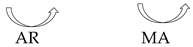
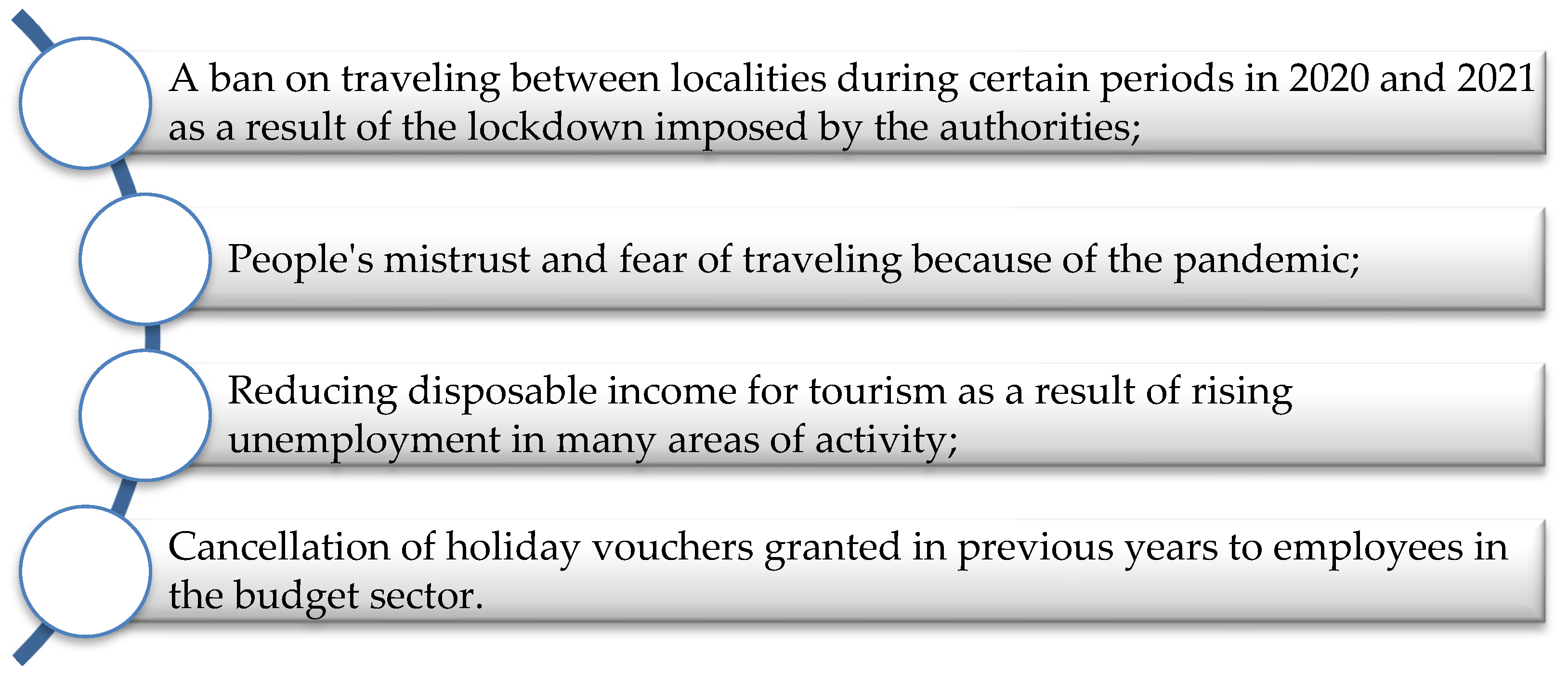
The COVID-19 pandemic has impacted a number of economic sectors, one of the most affected of which has been tourism. The causes that generated the sharp reduction in the tourism sector in Romania in the post-pandemic period are numerous, as shown in
Figure 1.
As a result of the reduction in both domestic and international tourist arrivals in Romania, and implicitly, of the reduced revenues obtained from tourism, it is particularly important for both tour operators and government institutions to forecast the future, short–medium-term evolution of tourist arrivals in order to estimate the future income that can be obtained from this sector. For this purpose, forecasting arrivals in Romania in the next period, we will look for the best model that can statistically approximate the evolution of this series of monthly data.
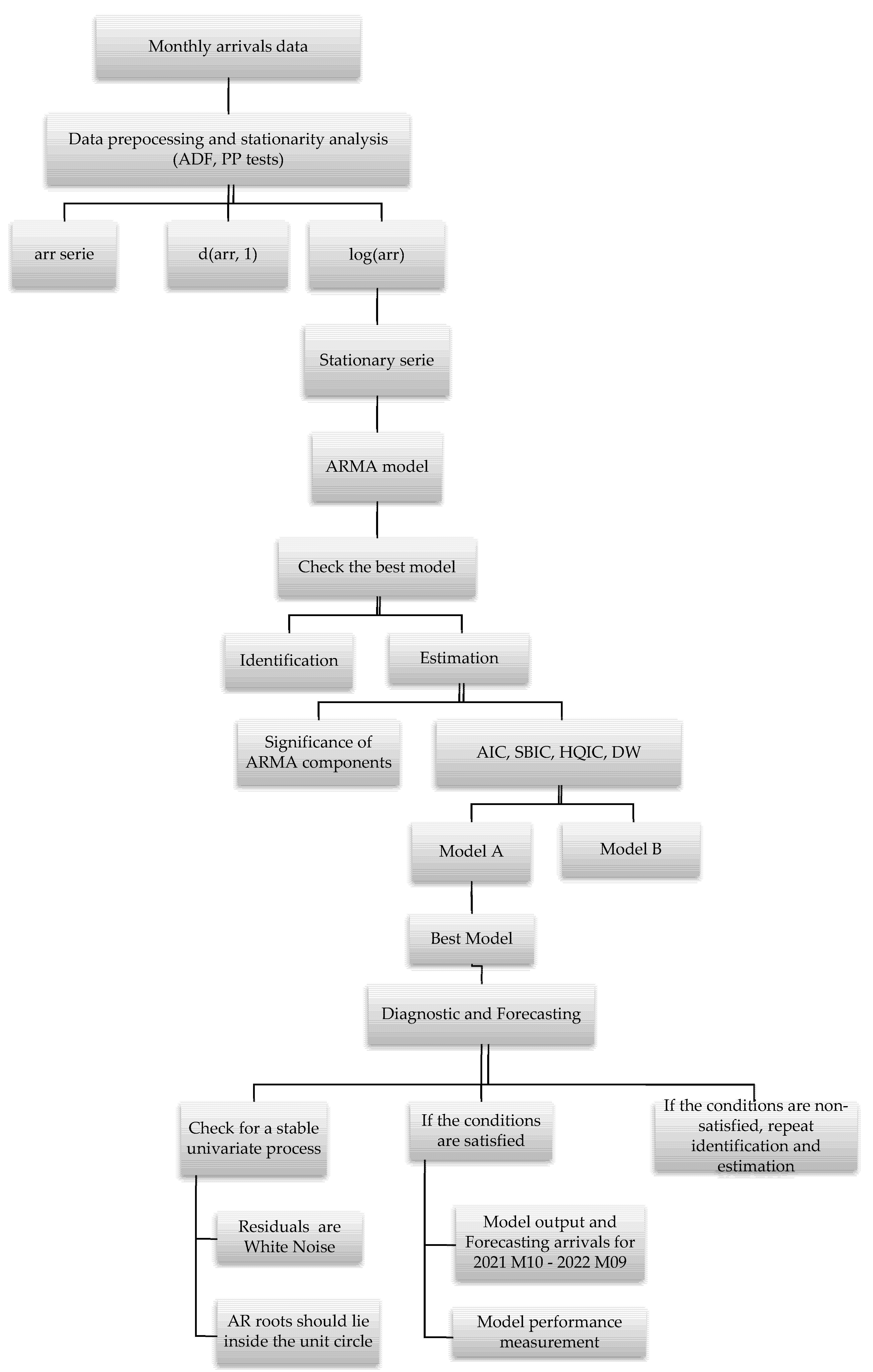
3.2. The Algorithm of the Forecast System of Arrivals in Romania in the Post-Pandemic Period
In order to choose a forecast model for arrivals, we followed the following algorithm for this study based on the methodology mentioned in
Figure 2.
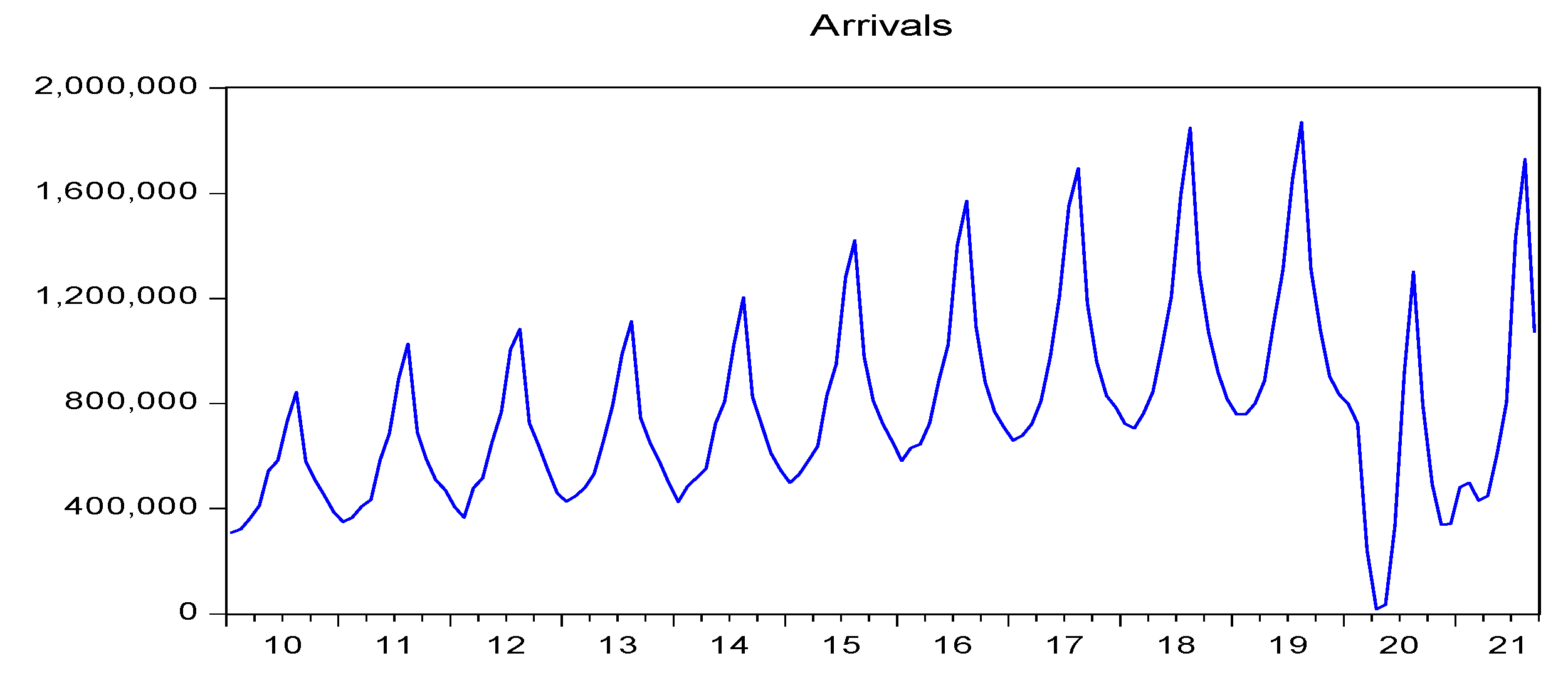
The evolution of the monthly series of arrivals for Romania between January 2010 and September 2021, based on statistical data obtained from the National Institute of Statistics of Romania,
www.insse.ro (accessed on 1 December 2021), is plotted in
Figure 3.
In order to choose a statistical forecast model for arrivals in Romania, it must meet certain conditions, which is why we started by studying the normality and stationarity of the
arr series, according to
Table 1.
Verifying the stationarity of the initial series
arr and the series
d (arr, 1) was performed using the auto-correlation function graph [
87] (ACF), partial auto-correlation function graph [
88] (PACF), as well as through the ADF [
89] test (augmented Dickey–Fuller) and PP [
90] (Phillips–Perron), and it was found that both series studied were not stationary. For this reason, we studied the stationarity of the
log(arr) series obtained by logarithmizing the initial series
arr, which proved to be stationary according to the ADF and PP tests, which allowed us to apply an ARMA model (
p, q).
The ARMA model attributed to Box–Jenkins (1970) can be applied in tourism forecasting for monthly number of tourist arrivals. The ARMA model used the order of the autoregressive (AR) model (p) and the order of the moving average (MA) model (q), called ARMA by the Box–Jenkin models (p, q).
“An ARMA based model has a significant advantage in terms of forecast accuracy. This magnitude of improvement in the accuracy of the model is likely to have a considerable positive effect on the quality of various managerial decisions made by hospitality industries and recreation manager” [
40].
ARMA is “an algorithm for the covariance determinant of a stationary autoregressive-moving average model is considered. Some asymptotic properties of this determinant in the stationarity and invertibility region of the process are studied numerically” [
91].
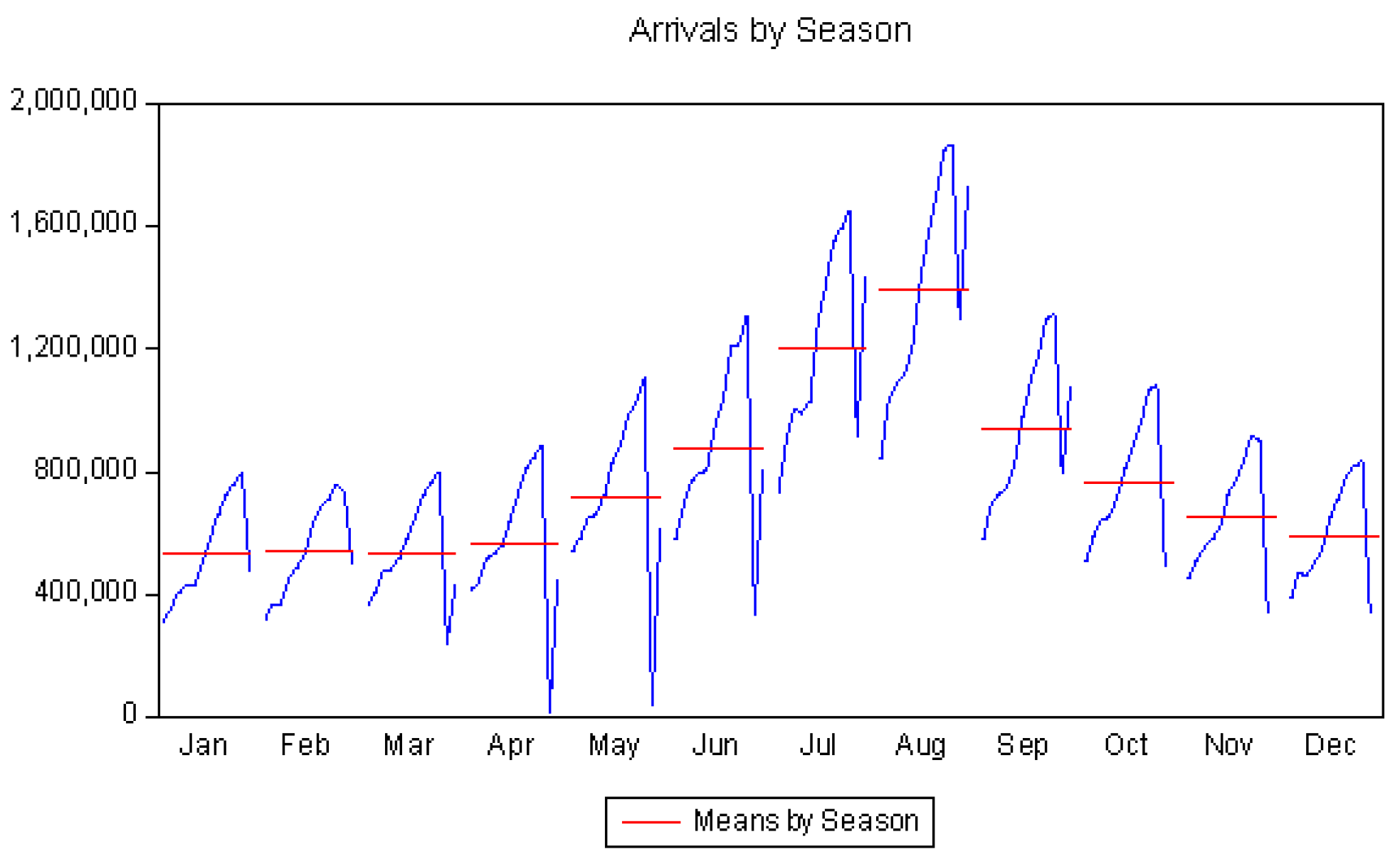
Given that tourism activity is seasonal (
Figure 4) in general, and that the logarithmic series is stationary, the Box and Jenkins test can be applied.
3.3. Methodology
The Box and Jenkins test (1970) for choosing a model for determining the prediction model involves three steps, namely: Identification, Estimation, and Diagnosis and Forecasting.
3.3.1. Identification
An ARMA model (p, q) is linear, and is obtained as a linear combination of two other linear models.
Based on the output of the ADF test, it is found that the probability associated with the constant c is 0.002, being less than the critical value 0.05, which means that this constant c must be included in the ARMA model.
Thus, for the stationary function log
(arr), we can write:
Based on the ACF and PACF correlogram for the log (arr) series, possible ARMA models are identified based on the lags that exceed the confidence bands for autocorrelation and partial correlation. Thus, it is found that the possible models are AR(1)MA(1) and AR(1)MA(2).
3.3.2. Estimation of Models
We tested the possible ARMA models, i.e., AR(1)MA(1) and AR(1)MA(2), to find a stationary and parsimonious model that fitted the data well. The model selection criteria were:
Significance of the ARMA components;
Comparing Akaike, Schwartz and Hannan–Quinn, and the smaller is better;
Comparing Durbin–Watson statistics, with a value closer to two being better.
Based on these criteria, it is found that the AR(1)MA(1) is the model that could be used to forecast the arrival of tourists from Romania.
3.3.3. Diagnosis and Forecasting
The requirements for a stable univariate process are:
Residuals of the model are white noise applied Ljung–Box Q statistic;
Null hypothesis: residuals are white noise;
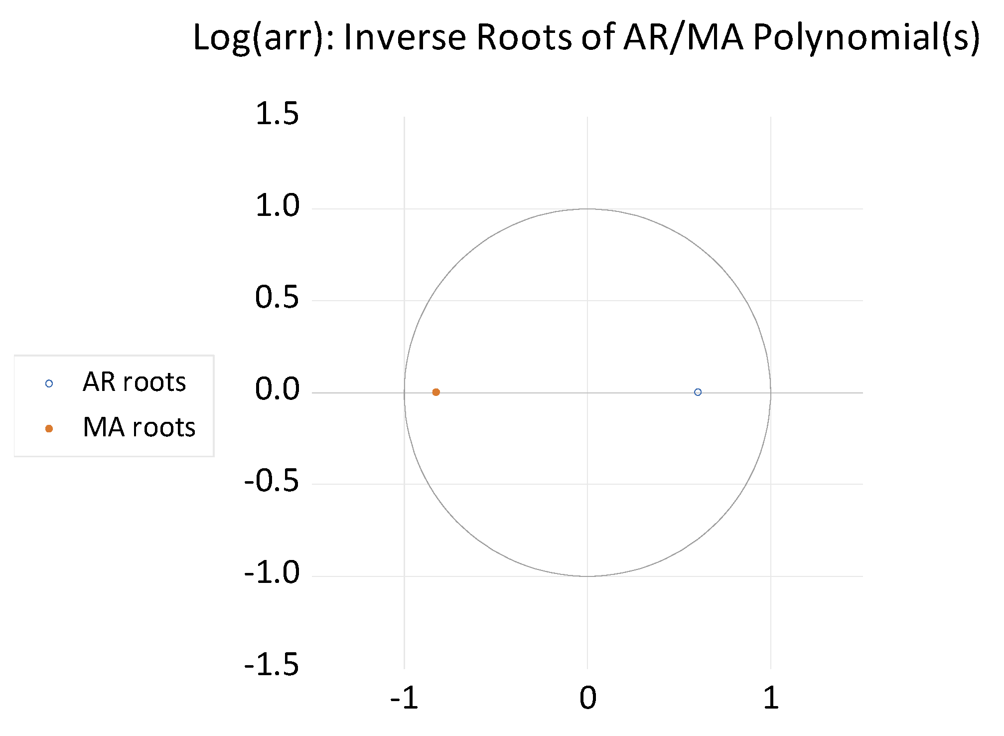
Check if the estimated ARMA process is (covariance) stationary: AR roots should lie inside the unit circle;
Check if the estimated ARMA process is invertible: all MA roots should lie inside the unit circle.
If the conditions are satisfied, we can forecast with this model and if the conditions are not satisfied, we need to repeat the selection and estimation method.
On AR(1)MA(1) all these conditions are met so we can move on to the next step, respectively we can forecast with this model AR(1)MA(1).
Additionally, if we proceeded with the automatic analysis of the forecast with ARMA model using the statistical program EViews, the whole model AR(1)MA(1) is determined automatically.
3.3.4. Forecast with the Chosen Model and Comparison with Statistical Data
Finally, the historical data for arrivals were compared with the forecast values from ARMA (1,1) which revealed a very good approximation. In conclusion, it can be chosen as forecast model for arrivals in Romania in the conditions of uncertainty generated by the COVID-19 pandemic is the ARMA model (1,1).
4. Results
4.1. Stationary Verification
To verify the stationarity of the series, we applied the ADF (augmented Dickey–Fuller) and PP (Phillips–Perron) stationarity tests, and we obtained the following results which showed us that the
arr and
d(arr,
1) series are not stationary, whereas the
log (arr) series is stationary. (
Table 2). Starting from H
0 (null hypothesis):
arr/d (arr)/log (arr) has a unit root; applying ADF and PP using EViews resulted in the following values in
Table 2.
Based on the results obtained by processing the series using the statistical software EViews for the centralized ADF and PP tests in
Table 2, for the series
arr and
d (arr, 1), H
0 cannot be rejected because the value of the test is higher than the critical value; thus, the series have a unitary root and they are non-stationary, for a relevance level of 1%. The same result is obtained if we analyze the probability associated with ADF and PP tests which is higher than the lowest level of relevance, namely, 0.01. Therefore, it can be stated that the hypothesis H
0 is accepted and that the series
arr and
d (arr,
1) have a unitary root; therefore, it can be stated that these series are non-stationary.
For the
log (arr) series, H
0 is accepted because the value of the statistical test is less than the critical value, for a relevance level of 1%. Therefore, we will choose the
log (arr) series because it is stationary and does not require differentiation, unlike the initial arrivals series which is not stationary even after the difference of order 1. Thus, we can say that the
log (arr) series is stationary, and that an ARMA model
(p,
q) can be applied because it does not need differentiation. Given that the probability corresponds to the
c constant in the ADF test, which is 0 < 0.05, we will include the
c constant in the ARMA model. Additionally, for the
log (arr) series the Durbin–Watson coefficient has a value of 1.927879 which is close to 2, which means that the parameters are stable, according to
Table 3.
4.2. Identification and Estimation
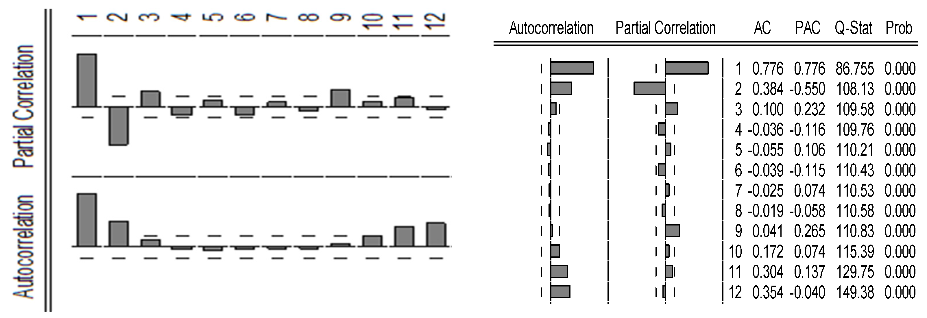
Based on the ACF and PACF correlation chart for the
log (arr) series in
Figure 5, possible ARMA models are identified based on the lags that exceed the confidence band for autocorrelation and partial correlation. Thus, it is found that the possible models are AR(1)MA(1) and AR(1)MA(2), according to
Figure 5.
The lags exceeding the confidence band for autocorrelation are 1 and 2, and for partial correlation, the lags exceeding the confidence band are 1 and 2. Thus, the possible values for p for AR are 1 or 2; those for q corresponding to MA are 1 and 2. Therefore, the possible models are AR(1)MA(1) and AR(1)MA(2). We tested the two possible ARMA models, namely:
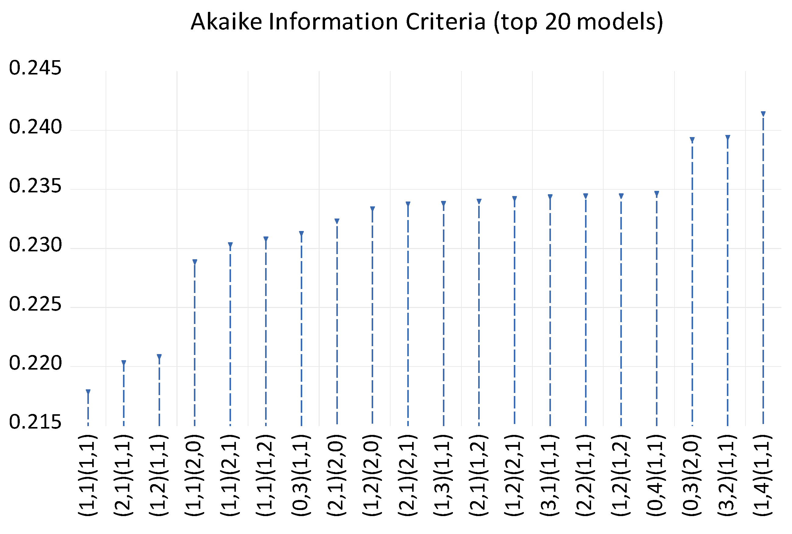
The best model must be stationary and parsimonious that fits the data well. Model selection criteria are: Sigma SQ, AIC (Akaike information criterion); SBIC (Schwarz Bayesian information criterion); HQIC (Hannan–Quinn information criterion); and Durbin–Watson (DW) statistics which are centralized in
Table 6, and according to which the best model is Model A, i.e., AR(1)MA(1).
Table 6 indicates best model: Sigma SQ, AIC: Akaike information criterion; SBIC: Schwarz Bayesian Information Criterion, HQIC: Hannan–Quinn information criterion and DW Durbin–Watson statistic.
4.3. Diagnosis and Forecasting
In order to determine whether the forecast can be made using the potential candidate model, Model A—AR(1)MA(1), we needed to test whether it meets the conditions to be considered a stable univariate process:
Hypothesis H0. Residuals are White Noise.
By applying Ljung–Box Q statistic for the potential model AR(1)MA(1), it is observed that the
p Value associated with the Q statistic > 0.05; thus, we cannot reject the null hypothesis, i.e., residuals are White Noise (
Table 7).
Check if the estimated ARMA process is (covariance) stationary: AR roots should lie inside the unit circle;
Check if the estimated ARMA process is invertible: all MA roots should lie inside the unit circle.
If the conditions are satisfied, we can forecast with this potential model AR(1)MA(1), but if the conditions are not satisfied, we need to repeat the selection and estimation method, according to
Table 8 and
Figure 6.
Thus, AR roots should lie inside the unit circle, and we can say the estimated ARMA process is (covariance) stationary, and although all MA roots should lie inside the unit circle, the estimated ARMA process is invertible.
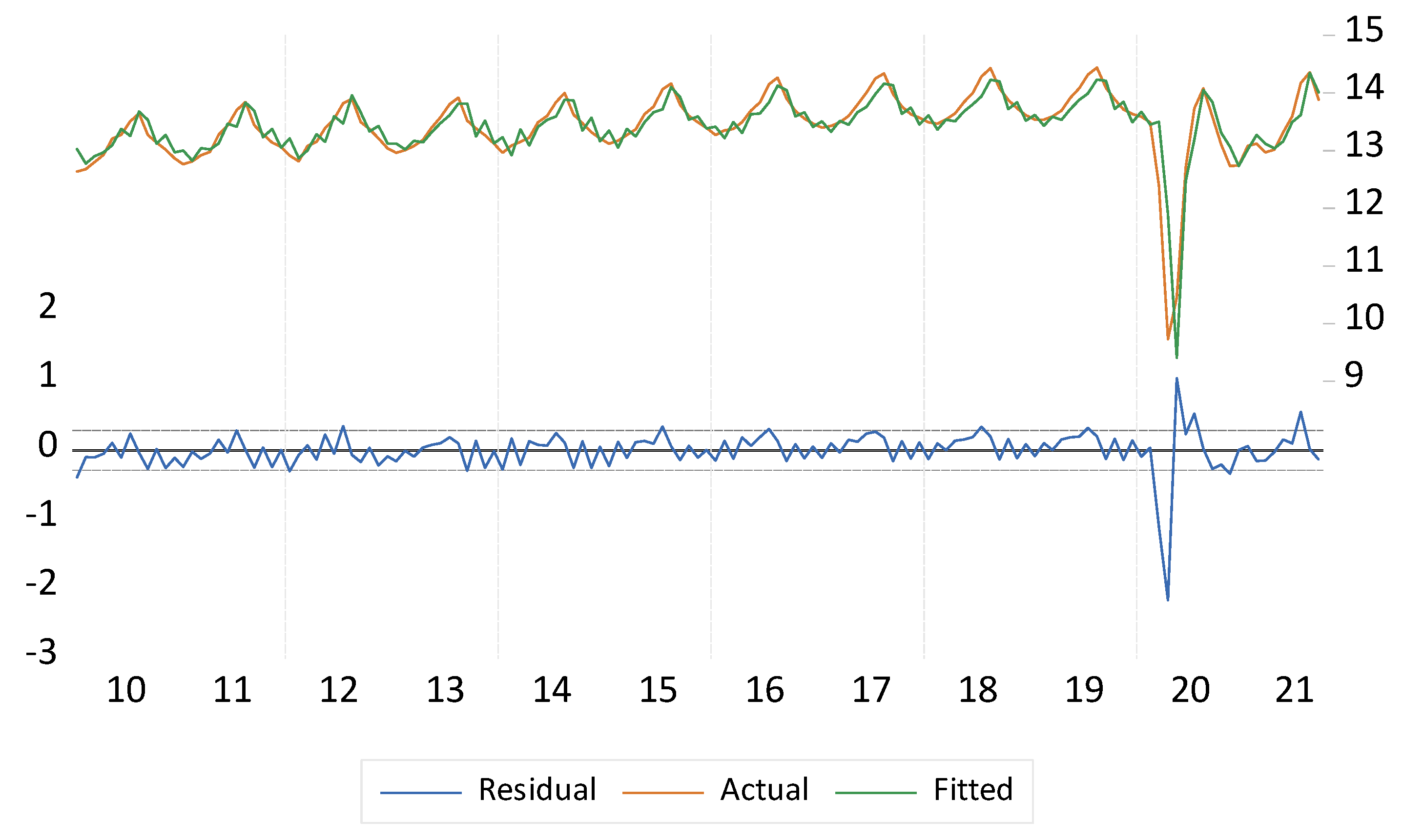
Thus, if the conditions are satisfied, we can forecast with the model AR(1)MA(1). It can be seen from
Figure 7 that the tested model AR(1)MA(1) approximates the past evolution very well, and that the residuals exceed the confidence interval only during the pandemic and post-pandemic periods, in 2020 and 2021, respectively.
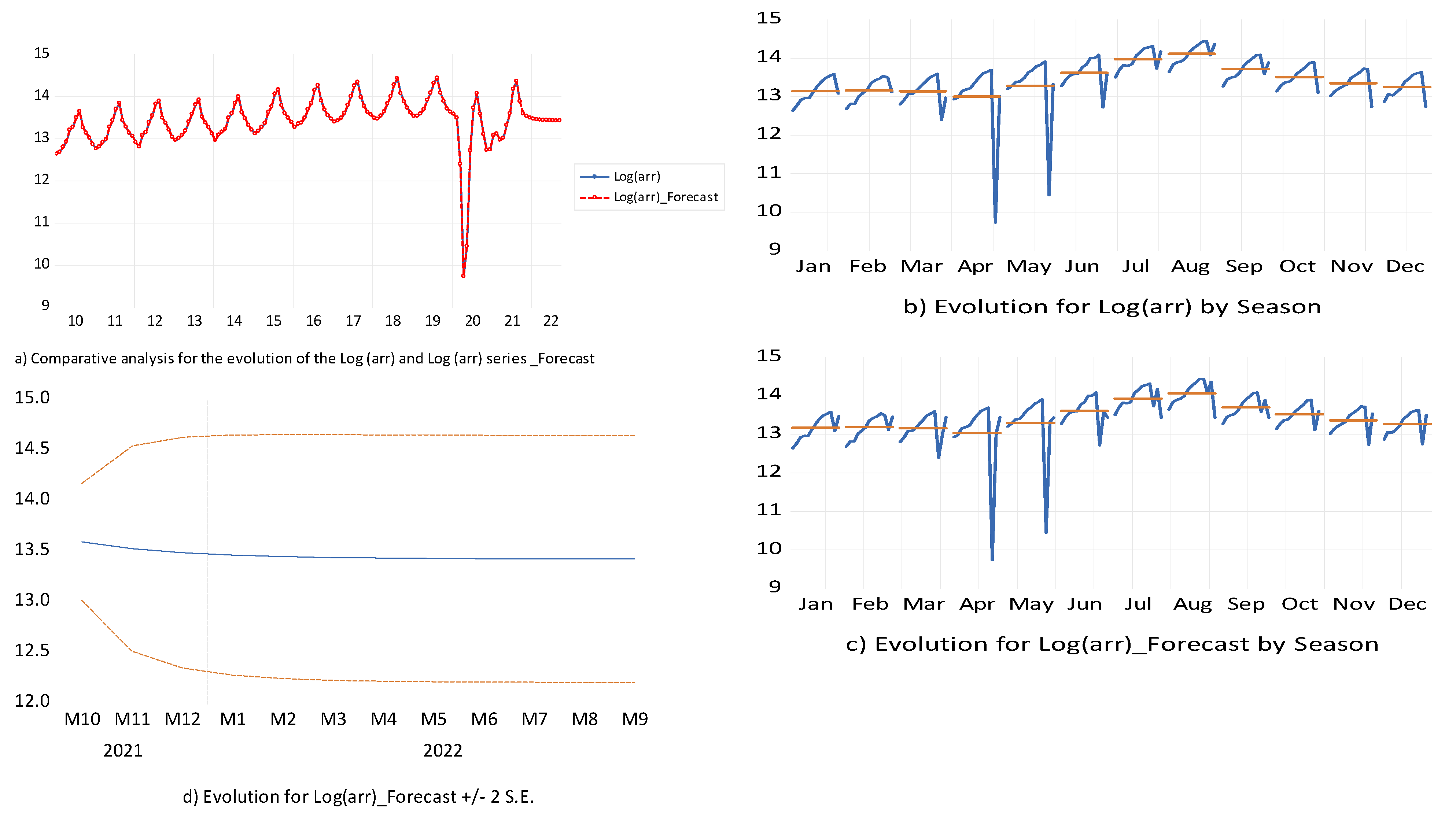
Forecast for the AR(1)MA(1) model can be seen in
Figure 8.
Based on the analyses in
Figure 8 and
Table 9, it can be seen that the chosen model of type AR(1)MA(1), on the basis of which the forecast for arrivals in Romania is made, perfectly approximates the previous evolution of arrivals.
This chosen model offers us the possibility to estimate the values of the flow of tourists from Romania, which is of great practical importance for the decision-making bodies in the field of tourism which can thus adapt their policies and strategies in the field of tourism according to these forecasted values to mitigate the negative effects of the current pandemic and uncertainty on Romanian tourism.
The existence of a model that predicts how tourist activity will evolve is very useful for adapting tourism policies according to the expected results that can be estimated for the next period.
Additionally, depending on the estimated values for the flow of tourists, it is possible to estimate the necessary personnel in the field and the correlation of the policies for establishing the quotas of migrants that can be employed in the tourism field, considering the fact that Romania is facing a personnel crisis in the field of tourist services.
5. Discussion
We have applied the ARMA method starting from the fact that the analyzed activity has a seasonal component, and the analyzed series regarding the tourist arrivals was not stationary.
Based on the studies performed, we found that the tourism phenomenon in Romania can be predicted using an AR(1)MA(1) model that accurately describes the previous evolution of the series of arrivals. The only deviations from the residuals for the forecast model from the confidence interval occurred during the pandemic, because due to the lockdowns, the tourism sector was particularly affected.
If we used only the computerized analysis of the tourism phenomenon in Romania with the help of EViews, it established that the best forecast model for the
arr series is also AR(1)MA(1) (
Table 10).
The criteria on the basis of which the forecast model is chosen by EViews software are given in
Table 11 and
Figure 9.
Starting from what is known as ARMA analysis, which is more an art than a science, because there is no perfect model or true model, we chose that model with which the forecast will be made only if the specialist considers that it meets the absolutely necessary requirements. Therefore, the automatic application of the methods offered by machine learning must be completed with an analysis assisted by a researcher who may or may not confirm the chosen model automatically.
In this paper, we have studied two ARMA-type models econometrically starting from the idea that the tourist activity is a seasonal and non-stationary one. Thus, through the comparative analysis of the models AR(1)MA(1) and AR(1)MA(2) we demonstrated that for the tourist flow in Romania can be forecast with the help of the model AR(1)MA(1), as we have searched a stationary and parsimonious model that fits the data well. Model selection criteria were: significance of the ARMA components, compare Akaike, Schwartz and Hannan–Quinn, and Durbin–Watson statistic. We found that the tourism phenomenon in Romania can be predicted using an AR(1)MA(1)-type model that meets the requirements for a stable univariate process and that it accurately describes the previous evolution of the series of arrivals. The only deviations from the residuals for the forecast model away from the confidence interval occurred during the pandemic, because due to the lockdowns, the tourism sector was particularly affected. We can say that for a short and medium time, the forecast with such a model is almost identical to reality.
In our study, the model automatically chosen by the software is the same as the one we found by reviewing the entire econometric methodology; therefore, the model with which we made the forecast for the tourist flow in Romania was the AR model (1) MA(1).
This paper is subject to study limitations, but may also suggest additional lines of research. This approach to tourism demand forecasting may continue in the future with interest for researchers by expanding the geographical area or pursuing tourism activity following this study, or may serve as a starting point for further research.
The tourism phenomenon is a very important field for Romania, and the effects generated by the COVID-19 pandemic on it are both social and economic, which is why a series of coherent measures are needed to resume and boost domestic tourism, as well as external tourism.
6. Conclusions
Tourism has been one of the sectors most affected globally due to the restrictions imposed during the COVID-19 pandemic, but also the reluctance of consumers to travel. Romania is no exception. Many holidays have been canceled during lockdowns and travel budgets have been tightened. As governments work to limit the spread of new, increasingly contagious strains of COVID-19, the tourism industry is hoping for an economic recovery. However, “green certificates” are not enough to relaunch tourism, which is only expected to return to pre-pandemic values in 2024.
The particularities of tourist services determine the fact there are many factors which influence the tourist demand, so that the prediction of the tourist demand becomes more complex and uncertain.
Knowing that the tourism system is affected, and it must respond to a growing number of global challenges, including the continuing uncertainty surrounding the health crisis and other challenges related to the market preferences of major tourism flows in emerging economies, new realities of mobility related to travel restrictions, the need for forecasting is necessary. In the hospitality industry, the idea that planning and forecasting activities are exclusively a function of management has been rejected. This appears at all levels, from the government downwards. Workers must consider the elements of the forecast so that the activity can be carried out successfully, but also the knowledge of how to predict market trends in order to be prepared for customer requests. During the COVID-19 pandemic, the global tourism industry suffered considerably, and many countries are trying to make forecasts and plans in order to recover tourism.
Tourism demand forecasting is a relevant and stimulating topic for various actors involved in the tourism sector, such as practitioners and policy makers. Access to good forecasts would help these agents anticipate future tourism demand and adapt their supply capacity conveniently, as well as optimize their human resources. Resources related to tourism could be allocated more efficiently, and the sector could produce more profit. For this reason, it is crucial for researchers and operational managers to choose a forecasting method that provides good predictive accuracy.
This study is apt because it addresses the severely affected tourist activity in a pandemic context, and it has both a theoretical applicability, by determining a model with which to predict the flow of tourists from Romania; and practically, it can estimate the values of tourist arrivals and enables the decision-making bodies in the field to take the necessary measures to mitigate the negative effects of the pandemic on this sector of the Romanian economy. For tourism decision makers, knowing a forecast of the trend for the flow of tourist arrivals in the short and medium term is useful for adopting strategies to support this field in the post-pandemic period. Additionally, the possibility to forecast the flow of tourist arrivals is useful for anticipating the necessary workforce in the field of tourist services.
The pandemic was a real shock for the Romanian tourism industry; therefore, we intend to study future if the reduction in the number of tourist arrivals was only temporary, being the manifestation of the shock, or whether the downward trend will continue in the future. We also intend to study in our future research on tourism activity whether the chosen model of type AR(1)MA(1) is suitable for other datasets, such as domestic or international arrivals.


 ,
, 


