Feature Extraction and Spatial Interpolation for Improved Wireless Location Sensing

Abstract

This paper proposes a new methodology to improve location-sensing accuracy in wireless network environments eliminating the effects of non-line-of-sight errors. After collecting bulks of anonymous location measurements from a wireless network, the preparation stage of the proposed methodology begins. Investigating the collected location measurements in terms of signal features and geometric features, feature locations are identified. After the identification of feature locations, the non-line-of-sight error correction maps are generated. During the real-time location sensing stage, each user can request localization with a set of location measurements. With respected to the reported measurements, the pre-computed correction maps are applied. As a result, localization accuracy improves by eliminating the non-line-of-sight errors. A simulation result, assuming a typical dense urban environment, demonstrates the benefits of the proposed location sensing methodology.

1. Introduction

Location-sensing Technology (LT) that enables the determination of a mobile device in a terrestrial wireless network is considered as the core of the future location-based Services (LBS) including route direction assistance, gaming, resource management, fleet tracking, security, location-based billing, and e-commerce. Since accurate, reliable, and secure provision of user position should be guaranteed for effective location sensing, there is an extensive literature dealing with the LTs. By investigating the open literature, it can be found that only a few LTs act as basis for many possible LBS applications.

Based on the source of signal, the currently-available LTs are basically classified into two groups: satellite-based methods and terrestrial network-based methods. The satellite-based methods based on the signals transmitted by GPS, GLONAS, or Galileo. The terrestrial wireless location systems are based on various types of network measurements including Time of Arrival (TOA), Time Difference of Arrival (TDOA), Angle of Arrival (AOA), and Signal Strength (SS). In spite of the accuracy benefits of satellite-based methods, considerable attention is paid to terrestrial network-based methods. The reason is that they utilize only generic network-oriented measurements, often do not require handset modification, are deployable where demand is greatest (e.g. in urban areas), and generally have a lower power consumption.

It is expected that most of requests for LBS would be invoked from urban environments. Unfortunately, most of network-based measurements suffer from Non-Line-Of-Sight (NLOS) error in dense urban areas. The NLOS error problem occurs when direct signal paths between mobile and base stations are mostly obstructed by buildings and other structures as shown in Fig. 1 so that the measured range information always contains positive error. It is likely that NLOS error can cause positioning errors of up to hundreds of meters in urban environments.

For the reason, extensive investigations have been carried out during the past decades to mitigate NLOS error using probability density function models [1], NLOS detection and de-weighting methods [2,3,4], constrained optimization methods [5,6,7], NLOS extraction at known positions [8], and database correlation method [9,10,11]. Each of the existing methods can be largely categorized into the filter-based method [1-7] and the survey-based method [8-11].

Among the two large categories of the NLOS mitigation methods, the survey-based method bears more possibility to improve practical positioning accuracy since it is based on real measurement statistics. The survey-based method consists of two phases; preparation phase and real-time service phase. In the survey-based methods, when a client's measurement arrives, it is correlated with the surveyed measurements to generate a distance (correlation) profile. A minimum (maximum) value appears in the distance (correlation) profile when a surveyed location is nearest to the client location. In the survey-based methods, achievable accuracy improves as the number of surveyed location increases. However, special instruments and extensive labor are required to get sufficient measurement statistics. In addition, computational burden to respond a client's location request increases as the number of surveyed locations increases. Fig. 2 illustrates the preparation and real-time service phases of the RF fingerprint technique. The RF fingerprint technique is the most representative technique among the conventional survey-based methods.

To eliminate the need for expensive outdoor surveys during the preparation phase and to reduce computational burden in responding location requests during the real-time service phase, this paper proposes a new methodology for efficient wireless location sensing. The proposed methodology, named as the Localization Exploring Network Measurement Occurances (LENMO), utilizes bulks of location measurements that are automatically collected from a wireless network. Investigating Signal Feature (SF) and Geometric Feature (GF) in each of the collected measurements, correction maps to mitigate NLOS error can be generated for an area where the measurements are collected. One example of the SF is the occurrence of the maximum signal strength values and several examples of the GF are road junction, corner, and special road geometry. Once the NLOS correction maps are generated, erroneous position estimates affected by the NLOS error, can be placed nearer to the true position.

Like the conventional survey-based methods, the proposed LENMO consists of two operational phases: preparation and service phases as shown in Fig. 3. However, during the preparation phase, a location server collects bulks of location measurements automatically instead of expensive outdoor surveys with extensive human labor. An additional important advantage of the proposed LENMO is that each of the collected location measurements does not need to utilize GPS.

To deal with the new localization methodology, this paper is composed as follows. In Section II, key concepts are explained including network structure, measurement sampling, data structure, reference information extraction, spatial processing algorithm, NLOS correction-map generation, and reference information exploration. In Section III, a simulation result under a Mahatan-like dense urban environment is presented. Finally, concluding remarks will be given.

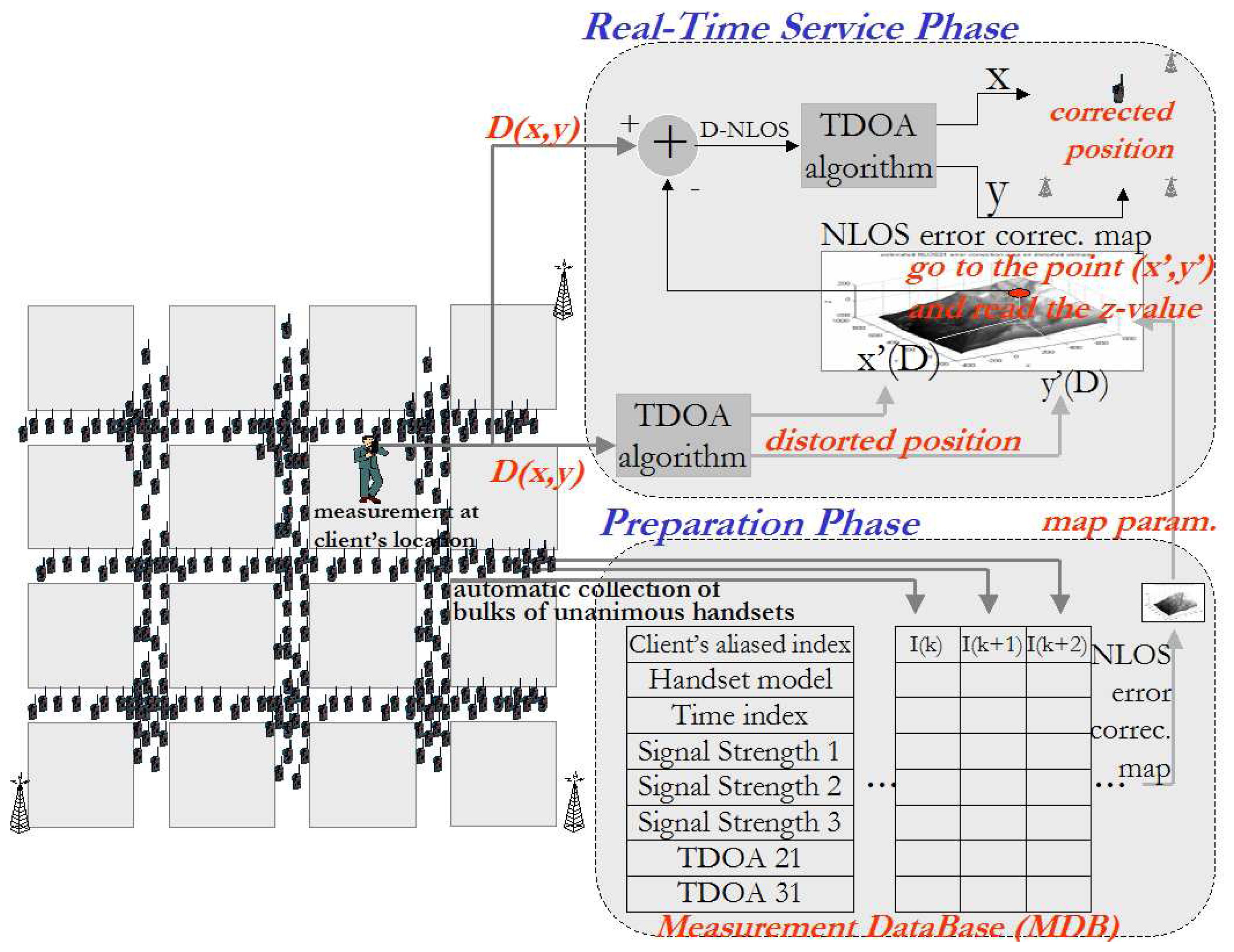
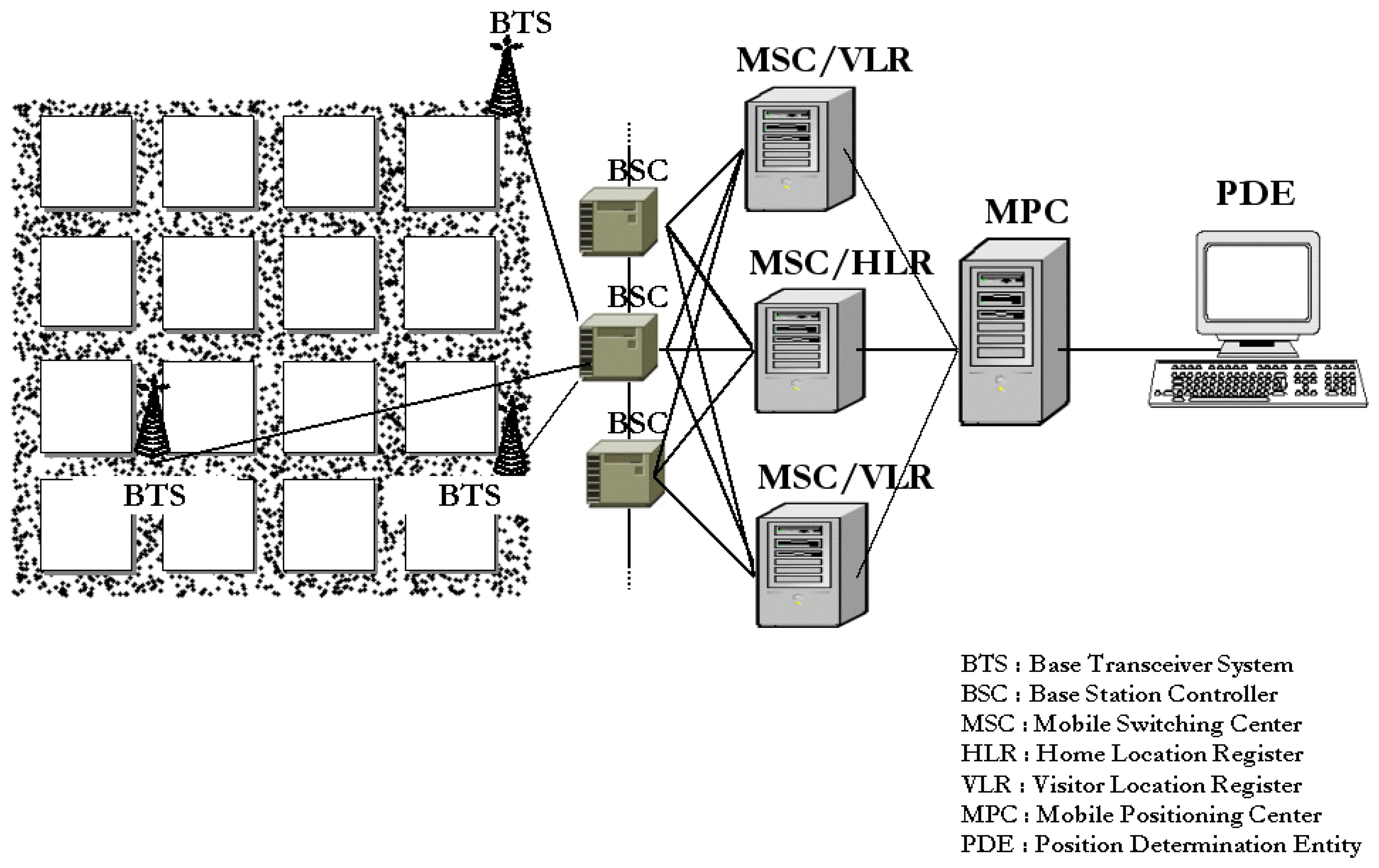
2. Localization Exploring Network Measurement Occurances

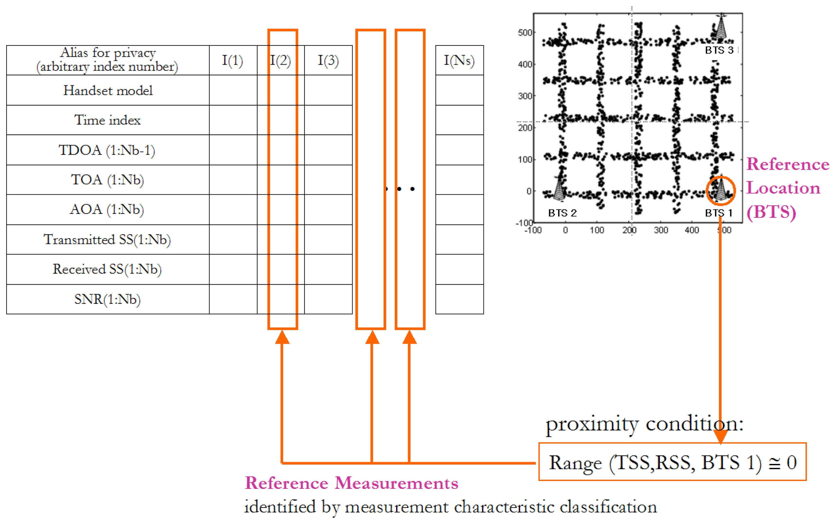
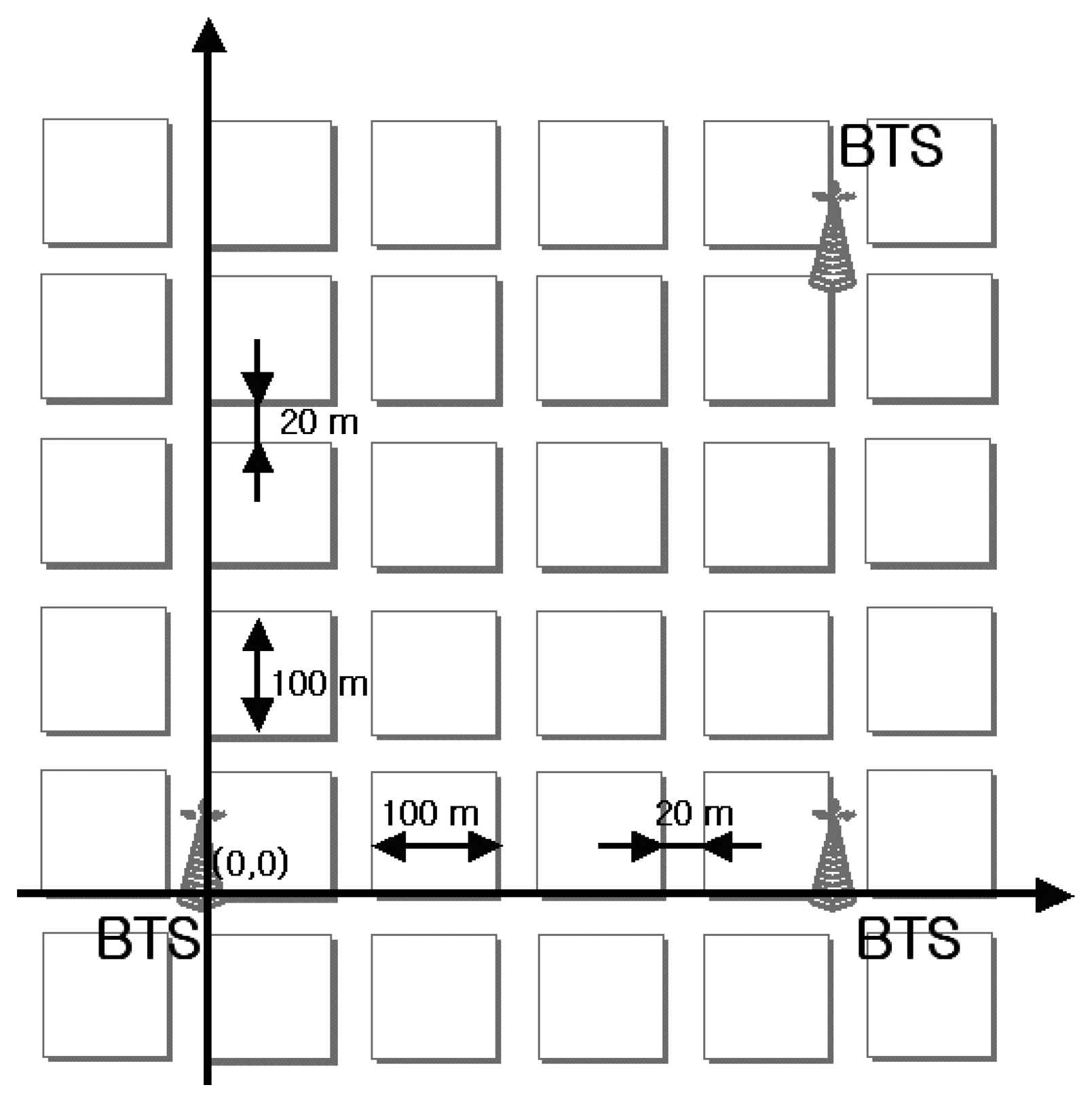
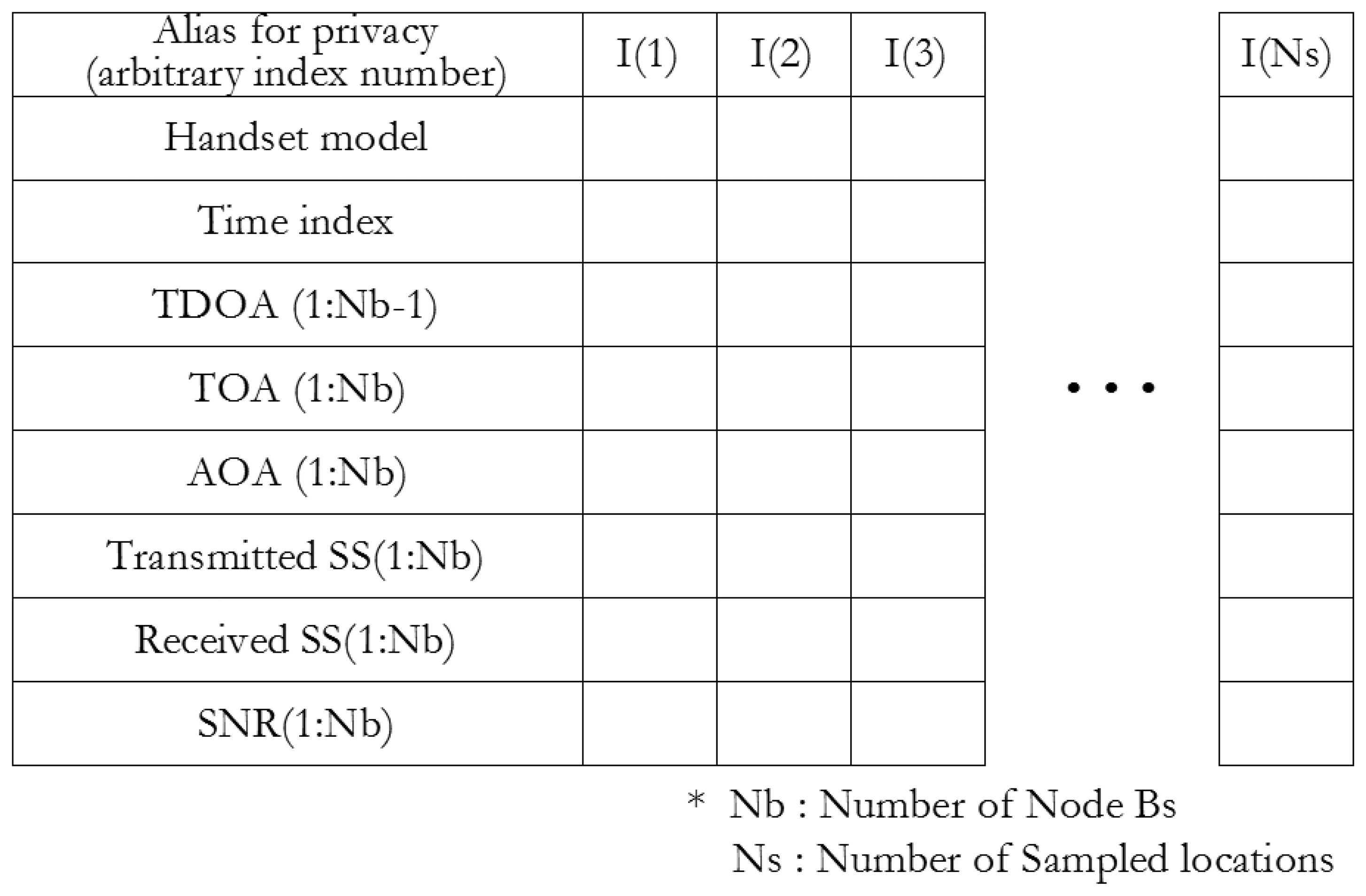
2.1. Measurement Sampling and Data Structure

The most important prerequisite for the proposed LENMO is the data structure for collected network measurements and the extraction of reference measurements from large amount of sampled measurements. Reference measurement extraction is obviously the key aspect of LENMO. Acquiring the reference measurements automatically can greatly facilitate the accumulation of the NLOS correction information [12]. The purpose of the data structure design is to facilitate efficient extraction of reference measurements from all the collected location measurements. Thus, a well-designed data structure should contain the data fields related to the timing, accuracy, and quality information for position estimation.

Fig. 4 shows a typical data structure for the proposed LENMO. As shown in Fig. 4, the data fields are categorized into user index, handset model, time index, and categorized location measurements. In the categorized location measurements, any type of the location measurement belonging to TOA, TDOA, AOA, Transmitted SS (TSS), Received SS (RSS), and Signal-to-Noise Ratio (SNR) can be included.

To indicate where to collect the location measurements, it is necessary to explain the architecture of Code Division Multiple Access (CDMA) standard [13-16]. Though the contents in this section mainly deals with the CDMA standard, similarities can be found under the Global System for Mobile Communication (GSM) standard [17-20] and many other descendants of the CDMA and GSM standards.

Fig. 5 shows a general arrangement of in a CDMA network. A Mobile Station (MS) corresponds to a user's wireless handset or mobile phone. A Base Transceiver System (BTS) is a network element that samples measurements of radio signals and communicates these measurements with the rest of the core network. A Base Station Controller (BSC) controls the signaling of the BTS serving each MS. An MSC (Mobile Switching Center) routes the calls bridging between the cellular network and other types of networks like internet. A PDE (Position Determination Entity) receives information from an MSC (control plane) or an MS (user plane) to estimate the location of the MS. The MSC invokes the PDE to initiate position determination.

A strong candidate platform on which the proposed LENMO can be implemented is the PDE in the core CDMA network. However, depending on circumstances, the proposed LENMO can also be implemented outside the core network if utmost care should be given to user index filed for privacy and anonymity. For this purpose, opaque ID, encripted ID, or randomly-generated temporary ID can be considered [20].

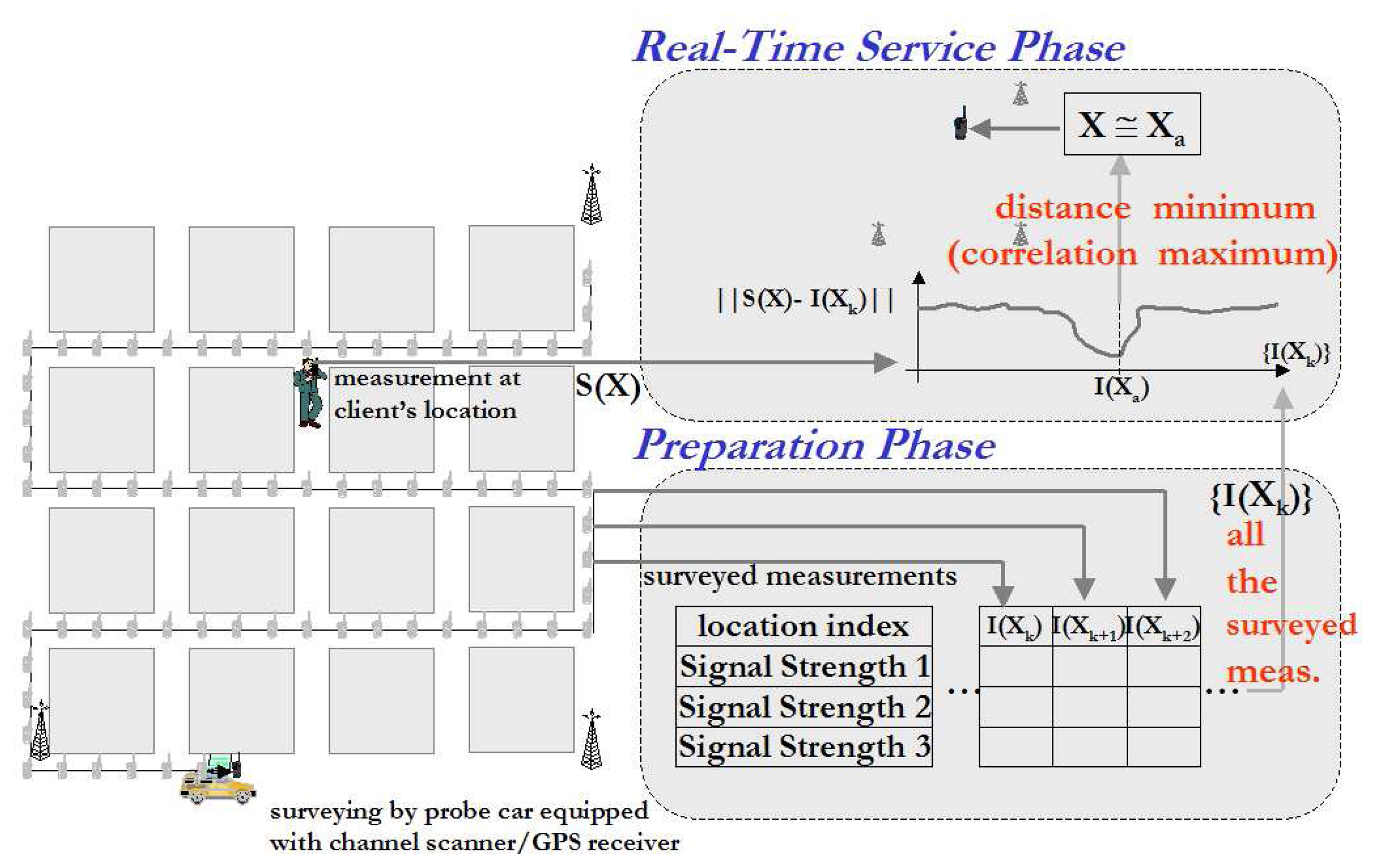
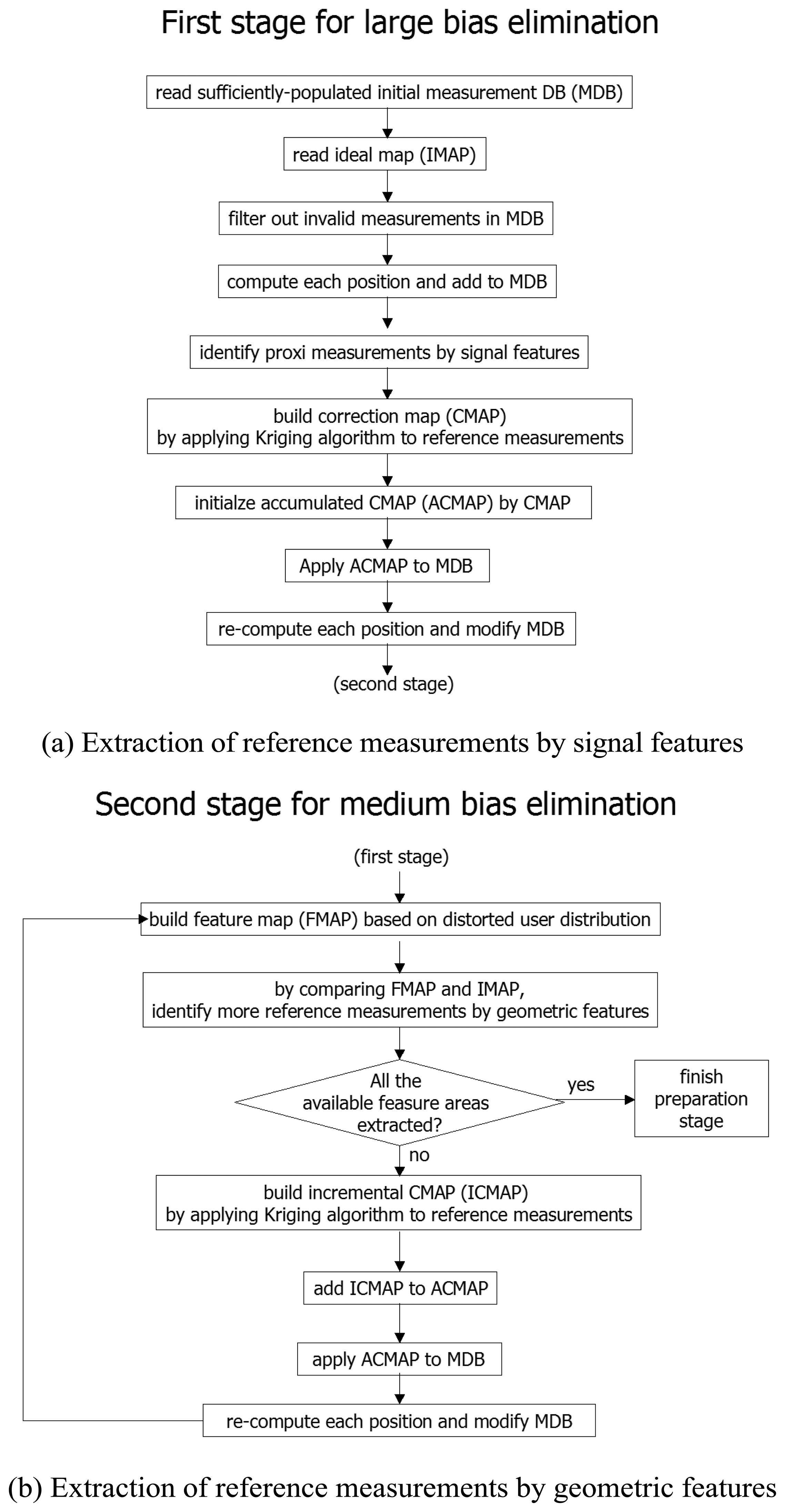
2.2. Reference Measurement Extraction

After sampling bulks of location measurements within a specific area of interest, it is necessary to filter out unnecessary measurements based on several data fields such as handset model, time index, and SS. During this step, measurements sampled from different hardware standards are filtered out by handset model. Additionally, if measurements sampled outside buildings are desired, measurements with small RSS/TSS ratio are filtered out. The remaining measurements after this step are stored in the Measurement DataBase (MDB) and utilized as the inputs to a typical positioning algorithm to obtain distorted user distribution as shown in Fig. 6.

Though any type of measurements among TOA, TDOA, AOA, and SS can be selected as the Major Measurement Type (MMT) in obtaining distorted user distribution, selecting the measurement type that occupies majority of the collected measurements as the MMT facilitates the processing thereafter. For illustration purpose, TDOA is considered as the MMT from now on. Given an initial position guess Xˆ = [xˆ ŷ]^T, J known BTS coordinates {X_j = [x_j y_j]^T} _j=12,…,J, (J - 1) TDOA measurements {d̃ _j1}_n=2,3,…,J, an estimate of position correction for more improved position estimate can be computed as follows [21].

$$X\Leftarrow X+\Delta X(\text{iteration})$$

(1)

where

$$\begin{array}{ll}\Delta X\hfill & ={(G^T{Q}^{-1}G)}^{-1}{G}^T{Q}^{-1}(\tilde{D}-\widehat{D})\hfill \\ \tilde{D}=\hfill & {\left[\begin{array}{cccc}{\tilde{d}}_{21}& {\tilde{d}}_{31}& \cdots & {\tilde{d}}_{J1}\end{array}\right]}^T\hfill \\ \widehat{D}=\hfill & {\left[\begin{array}{cccc}({\widehat{r}}_2-{\widehat{r}}_1)& ({\widehat{r}}_3-{\widehat{r}}_1)& \cdots & ({\widehat{r}}_J-{\widehat{r}}_1)\end{array}\right]}^T\hfill \\ G=\hfill & \left[\begin{array}{cc}\left(\frac{x_1-\widehat{x}}{{\widehat{r}}_1}-\frac{x_2-\widehat{x}}{{\widehat{r}}_2}\right)& \left(\frac{y_1-\widehat{y}}{{\widehat{r}}_1}-\frac{y_2-\widehat{y}}{{\widehat{r}}_2}\right)\\ \left(\frac{x_1-\widehat{x}}{{\widehat{r}}_1}-\frac{x_3-\widehat{x}}{{\widehat{r}}_3}\right)& \left(\frac{y_1-\widehat{y}}{{\widehat{r}}_1}-\frac{y_3-\widehat{y}}{{\widehat{r}}_3}\right)\\ ⋮& ⋮\\ \left(\frac{x_1-\widehat{x}}{{\widehat{r}}_1}-\frac{x_J-\widehat{x}}{{\widehat{r}}_J}\right)& \left(\frac{y_1-\widehat{y}}{{\widehat{r}}_1}-\frac{y_J-\widehat{y}}{{\widehat{r}}_J}\right)\end{array}\right]\hfill \\ \hfill & {\widehat{r}}_j=\Vert \widehat{X}-X_j\Vert \hfill \end{array}$$

(2)

and Q is the covariance matrix of the TDOA measurements. The Taylor-series algorithm described by Eqs. (1) and (2) produce reasonably accurate position estimates if the TDOA measurements are unbiased and the geometry condition represented by the observation matrix G is good.

If there is no NLOS error in the measurements, estimated user positions by a proper TDOA algorithm would be distributed in the neighborhoods of actual roads as shown by dark points of Fig. 6 though they are affected slightly by measurement geometry, noise, and fading effects. However, occurance of NLOS error is unavoidable in dense urban area where a lot of large buildings are present. The uncompensated NLOS errors in sampled measurements generate biased location estimates which constitute distorted user distribution compared with ideal map information.

To recover the distorted distribution to the ideal distribution, reference information is required. In the proposed LENMO, the reference information is formed by two features. One is SF and the other is GF. The utilization of SF is relatively simple. For this purpose, SS values of each measurements are checked. According to Hata –Okumura model [22] or COST 231 Walfisch-Ikegami model [23], SS value describes the distance between a transmitter and a receiver with good accuracy if they are sufficiently adjacent so that there is no obstruction for line-of-sight condition. Thus, the measurement set which includes the maximum SS with respect to some BTS means that they are sampled near that BTS as shown in Fig. 7. In these proxi-measurement sets, the effects of NLOS error would be small and their sampled position would approximately equals that of the corresponding BTS.

Usually, the amount of reference location measurements by SF would be too small to eliminate the distortion sufficiently. To provide sufficient amount of reference measurements, GF should be utilized. Dense urban area is mostly composed of road junctions, road segments, and buildings, where road junctions are stored as node, road segments are stored as links. If we consider a simple map that consists of nodes and links, any feasible map-matching techniques can be applied with respect to nodes, links, and node-link combined geometry [24]. Among the various combinations of nodes and links, a road junction which appears as a simple node, is the easiest feature to identify.

To extract reference measurements by map features, two maps are utilized; an Ideal MAP (IMAP) and a Feature MAP (FMAP). The IMAP is used as the reference information for LENMO. Thus, it should represent the real world accurately and includes the coordinates of BTSs, buildings, and geometric features such as road junctions and links as shown in Fig. 8. The FMAP is a 3-dimensional surface map based on distorted user distribution computed by the MDB. In the FMAP, z-values represent the degree of confidence of their corresponding xy-positions as feature areas. For example, the higher the z-value is, the more possible its xy-position corresponds to the a feature.

In Fig. 9, a two-step procedure building an FMAP representing smoothed population surface is illustrated. To compute the smoothed population surface as shown in Fig. 9(b), the distorted position domain is gridized by multiple rectangles. After gridizing the domain, the number of users in each rectangle is counted and saved as a gridized population surface. A road junction occupies more area than a road segment inside a rectangle of the same size. Thus, it can be easily understood that a rectangles with a road junction inside it contains more number of users assuming a uniform user distribution. Fig. 9(a) shows the gridized population surface constructed in this way. As shown in Fig. 9(a), road segments and road junctions can be recognized by non-zero height values though noisy. To eliminate noise fluctuations, a two-dimensional Gaussian filter algorithm [25] is applied to the gridized population surface. As a result, the smoothed population surface is obtained as shown in Fig. 9(b). As shown in Fig. 9(b), noisy fluctuations on the original population surface is eliminated where road junctions can be identified by local maximum peaks and road segments can be identified as the ridges between two local maximum peaks. By comparing the xy-positions of road junctions stored in the IMAP and the xy-positions with local maximum z-values in the FMAP, the distorted positions of road junctions are identified. For each identified xy-position of the FMAP, several reference measurement sets in the collected MDB can be found that corresponds to its neighbourhood. The identification of the reference measurements by GF is illustrated in Fig. 10.

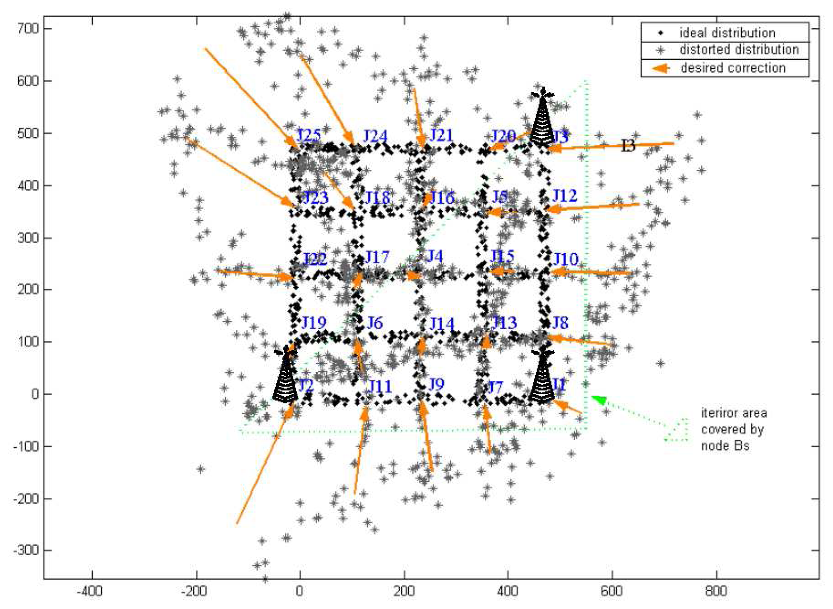
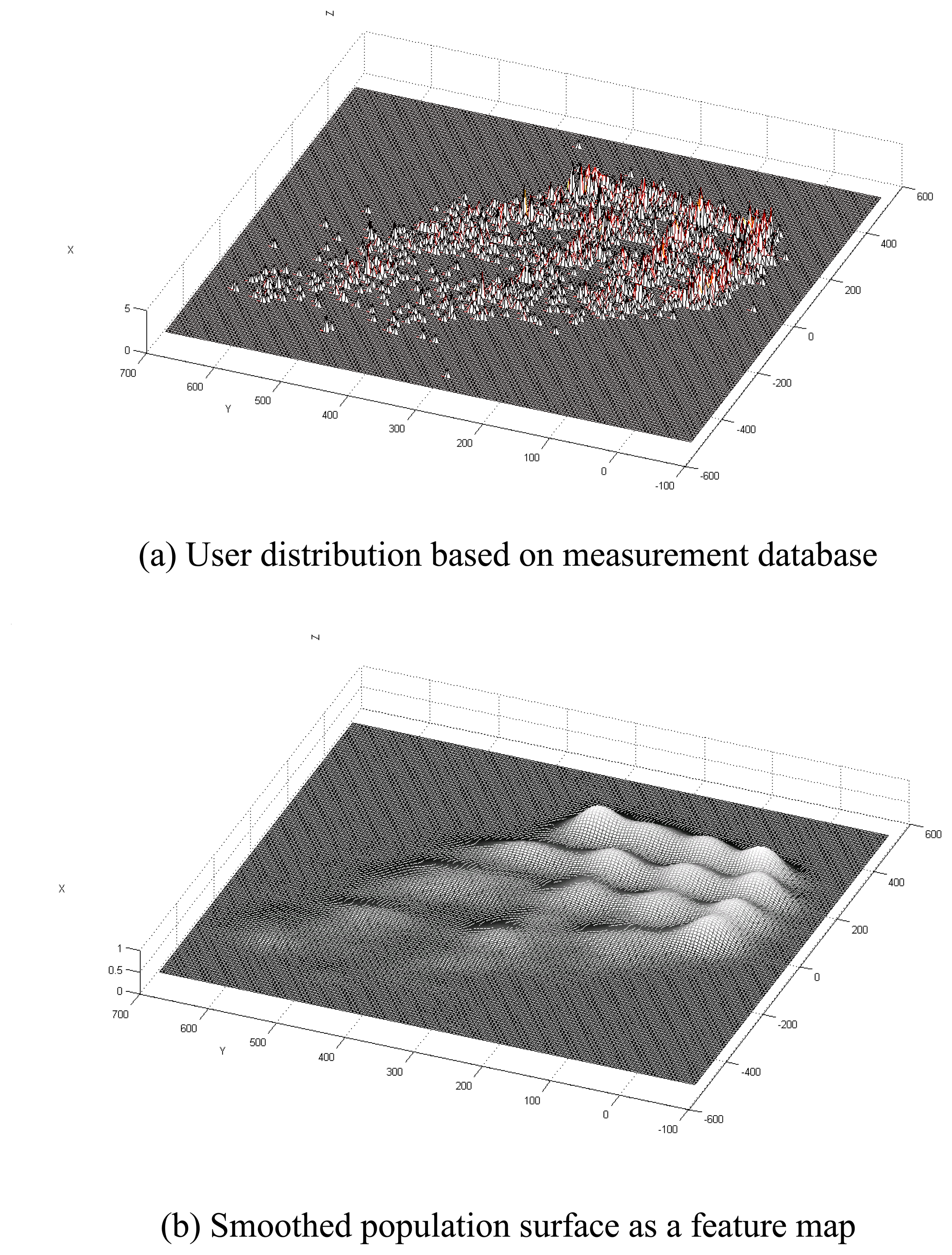
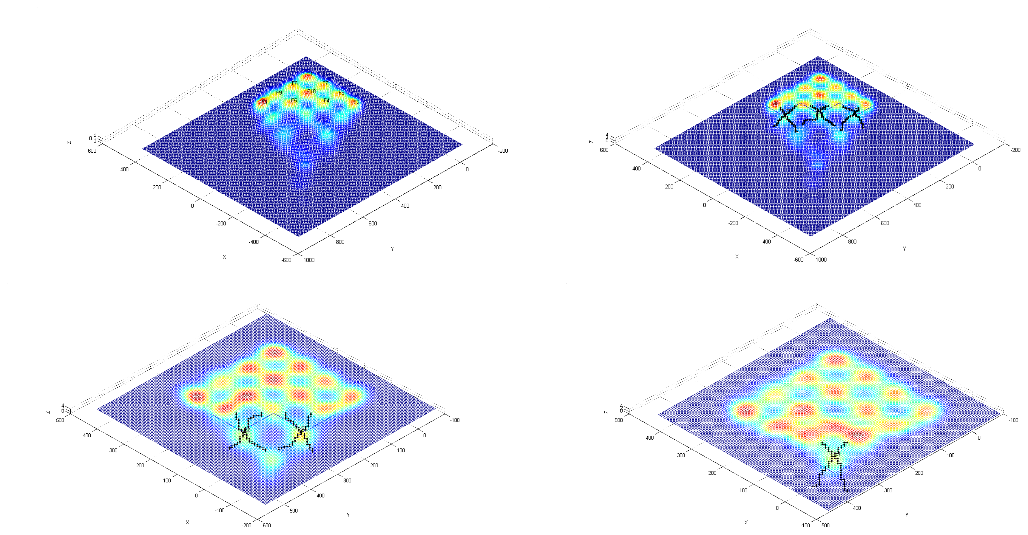
2.3. Spatial Interpolation

As explained before, reference measurements to mitigate map distortion can be extracted either by SF or by GF as shown in Fig. 7 and Fig. 10. Since each reference measurement is related to a point on ideal (undistorted) domain and a point on distorted domain, NLOS errors can be extracted as follows. Assume that a TDOA measurement _z(X) with its true position X = [x y]^T and distorted position X = [x̃ ỹ]^T is identified as the reference measurement. If we denote X_B1 = [x_B1 y_B1]^T and X_B2 = [x_B2 y_B2]^T as the known coordinates of BTSs, a TDOA measurement z(X) between BTS 2 and BTS 1 sampled at the reference location X satisfies the following relationship.

$$\begin{array}{l}z(X)=\Vert X-X_{B1}\Vert -\Vert X-X_{B2}\Vert +\mathit{\text{NLOS}}(X)+v(X)\hfill \\ \mathit{\text{NLOS}}(X)=h(X)\beta \hfill \end{array}$$

(3)

where β indicate the spatial structure of the NLOS error, h(X) is the observation matrix for β, and v(X) indicates the remaining smaller error sources.

If the spatial structure β of the NLOS error is known as a linear trend or a quadratic trend, h(X) and β in Eq. (3) can be rewritten as follows.

linear trend:

$$\begin{array}{c}h(X)≔[\begin{array}{ccc}1& x& y\end{array}],\\ \beta ≔{[\begin{array}{ccc}{\beta }_0& {\beta }_1& {\beta }_2\end{array}]}^T\end{array}$$

quadratic trend:

$$\begin{array}{l}h(X)≔[\begin{array}{llllll}1& x& y& x^2& y^2& \mathit{\text{xy}}\end{array}],\\ \beta ≔{[\begin{array}{llllll}{\beta }_0& {\beta }_1& {\beta }_2& {\beta }_3& {\beta }_4& {\beta }_5\end{array}]}^T\end{array}$$

(4)

In both cases, β₀ indicates the bias term in the spatial structure of NLOS error.

As shown in Eqs. (3) and (4), the NLOS error can be directly extracted at the reference locations where the related reference measurements exist. Unfortunately, no matter how densely reference measurements are identified, they cannot cover continuous area. To extract NLOS errors at arbitrary non-reference locations, the fact that adjacent two points show similar NLOS error characteristics is utilized.

To utilize the spatially correlated property of NLOS errors, any spatial interpolation algorithm such as nearest neighbor, inverse distance to a power, radial basis function, spline, Kriging, minimum curvature, polynomial regression, spatial Kalman filtering can be utilized [26-31]. Among the various spatial processing algorithms, Kriging is more attractive characteristics than others since it is based on well-developed statistical theory for spatial analysis. For modeling purpose, the measurement equation shown in Eq. (3) for reference locations is modified as follows.

$$\begin{array}{ll}\tilde{n}(X)\hfill & ≔z(X)-\Vert X-X_{B1}\Vert +\Vert X-X_{B2}\Vert \hfill \\ \hfill & =h(X)\beta +v(X)\hfill \end{array}$$

(5)

where ñ (X) indicates the newly defined NLOS measurement. By the Kriging algorithm, the estimate nˆ₀ of the NLOS error at arbitrary position X₀ given J reference measurements {ñ(Xˆ_j)}_j=1,2,…,J can be obtained as follows:

$$\begin{array}{ll}\widehat{\beta }=\hfill & {(H^T{C}_1^{-1}H)}^{-1}{H}^T{C}_1^{-1}\tilde{N}\hfill \\ \hfill & \widehat{n}(X_0)=c_0^T{C}_1^{-1}\left[\widehat{N}-H\widehat{\beta }\right]+h(X_0)\widehat{\beta }\hfill \end{array}$$

(6)

where

$$\begin{array}{ll}H≔& \begin{array}{cccc}\left[\begin{array}{c}h(X_1)\\ h(X_2)\\ ⋮\\ h(X_J)\end{array}\right],& \tilde{N}≔\left[\begin{array}{c}\tilde{n}(X_1)\\ \tilde{n}(X_2)\\ ⋮\\ \tilde{n}(X_J)\end{array}\right],& c_0≔\left[\begin{array}{c}\gamma (X_0,X_1)\\ \gamma (X_0,X_2)\\ ⋮\\ \gamma (X_0,X_J)\end{array}\right],& C_1≔\left[\begin{array}{cccc}\gamma (X_1,X_1)& \gamma (X_1,X_2)& \cdots & \gamma (X_1,X_J)\\ \gamma (X_2,X_1)& \gamma (X_2,X_2)& \cdots & \gamma (X_2,X_J)\\ ⋮& ⋮& \ddots & ⋮\\ \gamma (X_J,X_1)& \gamma (X_J,X_2)& \cdots & \gamma (X_J,X_J)\end{array}\right]\end{array}\\ & \gamma (X_i,X_j)=\frac{1}{2}Var\left[v(X_i)-v(X_j)\right]:\text{Variogra}m\end{array}$$

(7)

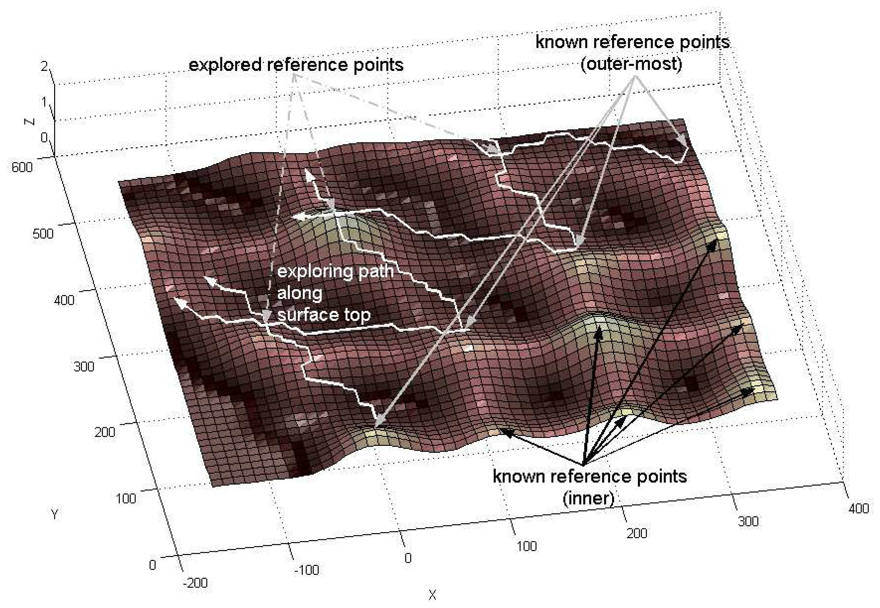
2.4. Exploration of More Reference Measurements

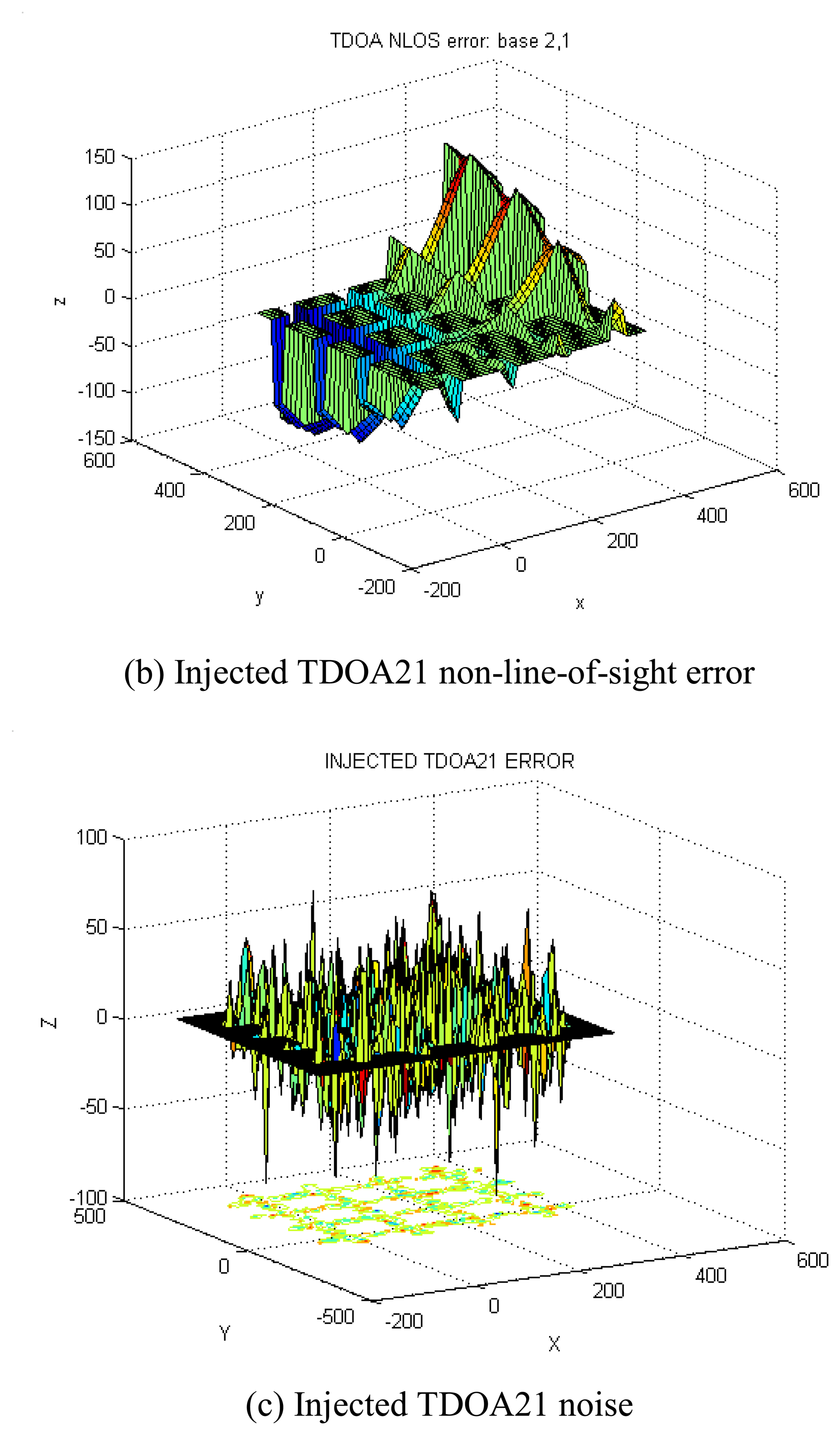
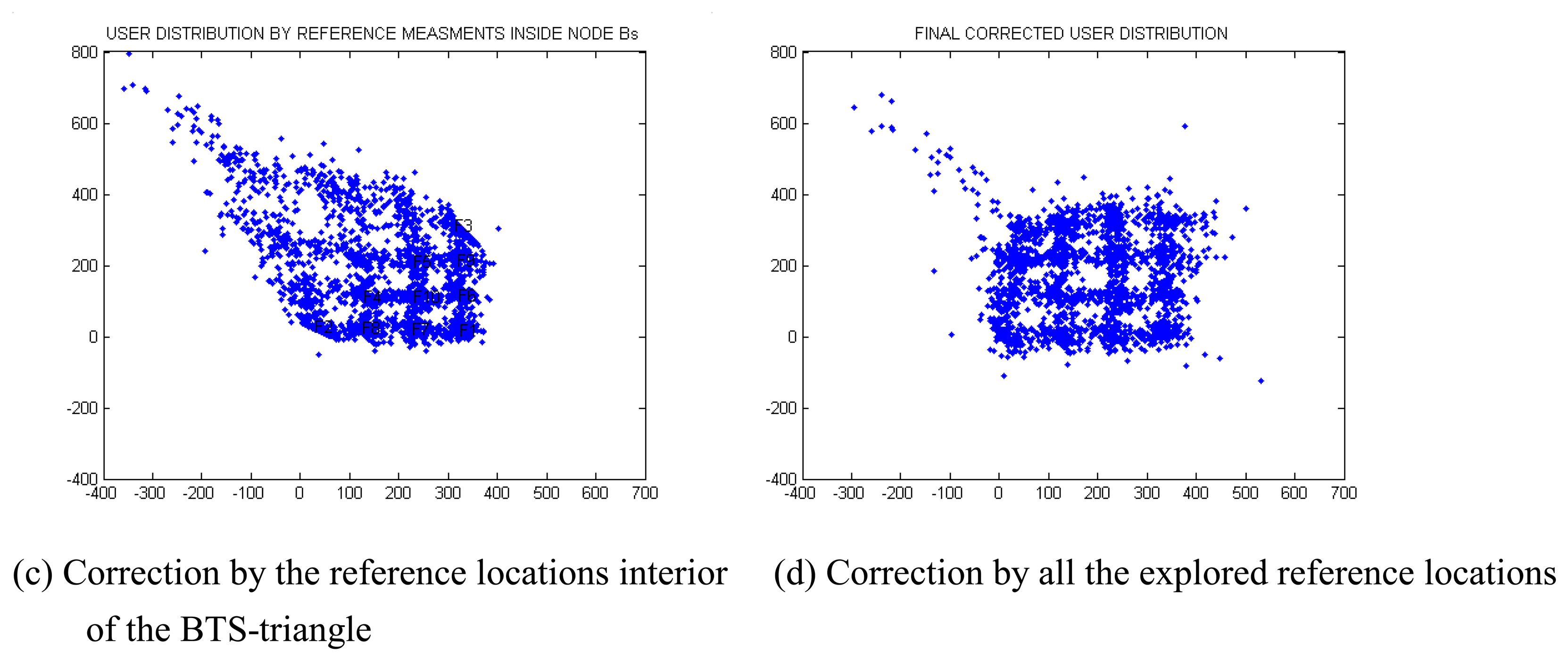
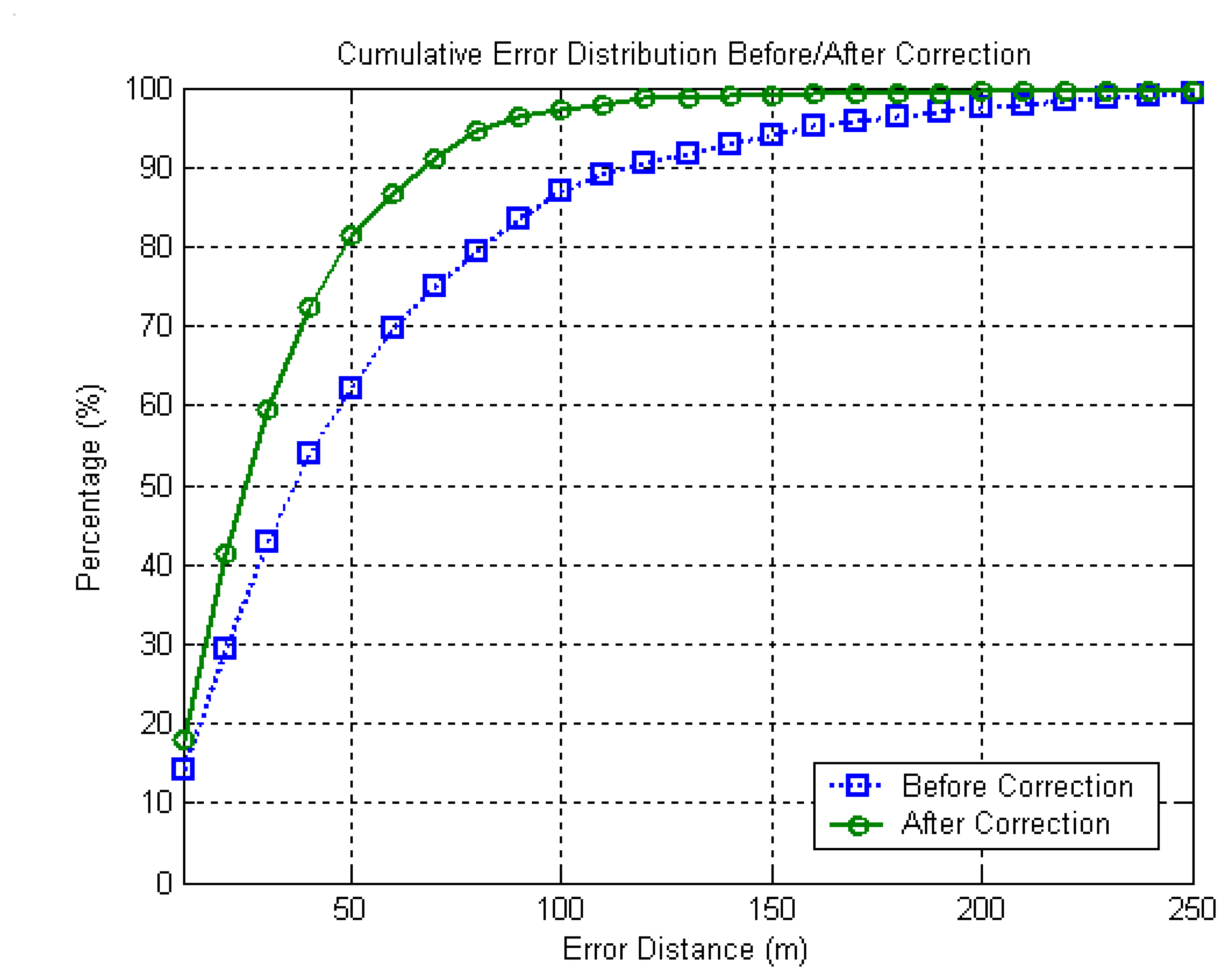
If the number of identified reference locations are sufficient, one trial of LENMO would be sufficient to correct NLOS effects. In most cases, however, the identification of all the reference locations by one trial of LENMO is difficult due to large effects of NLOS error, measurement geometry, and other noise effects. In these cases, it is necessary to expand the knowledge of reference locations step by step based on feedback structure.

For this purpose, all the possible reference locations in ideal map need to be arranged according to the identification convenience. The identification convenience is mainly affected by the measurement characteristic, geometry, and error magnitude. In Fig. 6, an arrangement scheme of reference locations is demonstrate. The reference locations J1-J3 correspond to the positions where BTSs are established and the reference locations J4-J15 and J16-J25 correspond to the interior and exterior area of the triangle made by three BTSs, respectively. The interior and exterior reference locations are indexed according to their dilution of precision values that explain geometric effects of BTSs.

By investigating the SS of a measurement set for SF, it is easy to determine if the set was sampled at the neighborhood of BTSs or not. After the identification, NLOS errors at the neighborhoods of BTSs are extracted. By utilizing the extracted NLOS errors as reference measurements, a large-scale NLOS correction map (CMAP) can be estimated by the Kriging algorithm. The CMAP generated after each identification procedure during the preparation stage corresponds to the partial correction information. To obtain the total correction information, each CMAP is summed up into an accumulated CMAP (ACMAP) as soon as it is estimated. During the service phase, the ACMAP is applied to all the stored measurement sets. The algorithm flow at this stage is described in Fig. 11-(a).

Re-computing user positions based on the ACMAP obtained at the first stage, a less distorted distribution map is obtained. In the beginning of the second stage of the LENMO algorithm, a smoothed population surface is constructed for the first time. All the local maximum points are compared with the corresponding reference locations in the ideal map as GF. Utilizing the reference measurements close to the identified inner reference locations, the NLOS error at each inner reference locations are extracted.

By utilizing the extracted NLOS errors as reference locations, an incremental CMAP (ICMAP) can be estimated by the Kriging algorithm. By adding the ICMAP to the ACMAP of previous stage, a newly updated ACMAP is obtained. By applying the ACMAP to all the stored TDOA measurements and re-computing user positions again, a much less distorted distribution map is obtained. At this stage, the NLOS errors inside the BTS-triangle are mostly eliminated. The algorithm flow at this stage is described in Fig. 11-(b).

For network management efficiency, BTSs are usually installed as uniform as possible in dense urban area. In this case, most user locations can be assumed to lie inside a triangle defined by three BTSs. If it is not the case, the exterior reference locations should be explored utilizing the interior reference locations. For this purpose, the algorithm flow shown in Fig. 11-(b) can also be utilized.

Usually, an ideal map representing dense urban environment is composed of nodes and links where nodes represent road junctions and links represent road segments connecting two road junctions. Each link can be considered as one line segment of a rectangle that corresponds to a building or a group of buildings. For the reason, any two different links on a map are usually parallel or orthogonal. Utilizing this characteristic, an efficient reference location exploration strategy can be devised.

The key idea to explore more reference locations is illustrated in Fig. 12 where the inner reference locations, the outer-most reference locations, and the explored points are depicted. As shown in Fig. 12, an explored points is found by finding the cross point of two exploring paths that originate from two outer-most reference locations. The exploring paths follow the ridges originating from outer-most reference locations.

3. Simulation

To verify the effectiveness of the proposed LENMO, a simulation was performed. Since SS values drop largely if wireless signals penetrate building walls, the measurement sets corresponding to the interior of buildings can be effectively filtered out. For the reason a uniform user distribution on road segments in a Manhattan-like urban environment can be generated, as shown in Fig. 13-(a). To generate the true TDOA, three BTS locations are assumed as indicated in Fig. 13-(a). By adding the NLOS error and noise terms to the true range difference, the TDOA measurements are generated. The standard deviation of the white noise added to each TDOA measurement is set as 30 meters. Since three BTSs are established, two TDOA measurements representing TDOA21 and TDOA31 are available for each point in Fig. 13-(a). Figs. 13 and 13-(c) depict the injected NLOS error and noise values. Because of the injected NLOS error and noise, the position estimates based on the TDOA measurements do not fit the well-arranged distribution shown in Fig. 13-(a), but rather to the severely-distorted distribution in Fig. 14-(a).

By applying the LENMO based on the reference measurements near the BTSs, a less distorted user distribution as shown in Fig. 14-(b) is obtained. In identifying the reference measurements near the BTSs, the SS values that indicate the range information from BTSs are utilised as SF indicator.

After the smoothed population surface of the user distribution is constructed as shown in Fig. 14-(b), its local maximum points are compared to the road junction points on the ideal map. As a result, the reference measurement sets that correspond to the internal area of the BTS-triangle are identified by GF. By applying the LENMO based on the identified reference measurements, a less distorted user distribution, as indicated in Fig. 14-(c), is obtained.

After the smoothed population surface of the user distribution of Fig. 14-(c) is constructed, the remaining exterior reference locations are explored outside the BTS-triangle by adopting the strategy explained in sub-section 2.4. As soon as any new reference locations are explored, the LENMO algorithm is applied to obtain the updated smoothed population surface. By iterating this procedure, all the reference locations are found and the resulting user distribution is obtained as shown in Figure 14-(d). By comparing Figs. 14-(a) and 14-(d), it can be seen that the proposed LENMO is quite effective. The overal exploring procedure is depicted in Fig. 15. By Figs. 14 and 15, it is apparent that the proposed LENMO is quite effective in reducing the effects of NLOS errors.

To provide an insight into how much effective the proposed LENMO is, error distances between estimated and true user positions are computed. The cumulative error distribution diagram of Fig. 16 is obtained. The two lines with symbols ‘o’ and ‘+’ correspond to the cumulative error distribution before and after the NLOS error correction, respectively. As indicated in Fig. 16, the error distance reduces from 117.1 meters to 67.4 meters for the probability of 90%. This result means that the location errors are reduced to almost 57 %.

4. Conclusions

An efficient location sensing methodology is proposed for calibrating non-line-of-sight error in urban environments. The proposed methodology utilizes automatically collected measurements from a wireless network infrastructure. After the identification of feature locations by signal and geometric features, the non-line-of-sight error correction maps are generated. For real-time implementation, the pre-computed correction maps can be utilized for more accurate and fast localization. To explain the proposed methodology in detail, various key concepts are introduced including network structure, measurement sampling, data structure, reference information extraction, spatial processing algorithm for NLOS correction-map generation, and reference information exploration. A simulation result demonstrated how location accuracy improves gradually by the proposed methodology.

References and Notes

1. Morley, G.; Grover, W. Improved location estimation with pulse-ranging in presence of shadowing and multipath excess-delay effects. Electron. Lett. 1995, 31(18), 1609–1610. [Google Scholar]
2. Wylie, M.; Holtzman, J. The nonline of sight problem in mobile location estimation. IEEE Int. Conf. Universal Personal Communication 1996, 827–831. [Google Scholar]
3. Chen, W. A cellular based mobile location tracking system. 49th IEEE Vehicular Technology Conf. 1999, 3, 1979–1983. [Google Scholar]
4. Xiong, L. A selective model to suppress NLOS signals in angle-of-arrive (AOA) location estimation. 9th IEEE Int. Symp. Personal, Indoor and Mobile Radio Communication 1998, 1, 461–465. [Google Scholar]
5. Caffery, J.J.; Stuber, G. Subscriber location in CDMA cellular networks. IEEE Trans.Veh. Technol. 1998, 47, 406–416. [Google Scholar]
6. Kim, W.; Lee, J.G.; Jee, G.I. Direct estimation of NLOS propagation delay for mobile station location. Electronics Letters 2002, 38(18), 1056–1057. [Google Scholar]
7. Wang, X.; Wang, Z.; O′Dea, B. A TOA-Based Location Algorithm Reducing the Errors Due to Non-Line-of-Sight (NLOS) Propagation. IEEE Trans.Veh. Technol. 2003, 52, 112–116. [Google Scholar]
8. Watters, J.M.; Strawczynski, L.; Steer, D. Devices and processing in a mobile radio communication network having calibration terminals. US patent 6,230,018, 2001. [Google Scholar]
9. Wax, M.; Hilsenrath, O. Signature Matching for Location Determination in Wireless Communication Systems. U.S. Patent 6,112,095, 2000. [Google Scholar]
10. Laitinen, H.; Nordstrom, T.; Lahteenmaki, J. Database Correlation Method for GSM Location. Proceedings of IEEE Vehicular Technology Conference 2001, 4, 2504–2508. [Google Scholar]
11. Li, B.; Wang, Y.; Lee, H.K.; Dempster, A.; Rizos, C. Method for yielding a database of location fingerprints in WLAN. IEE Proceedings-Communications 2005, 152(5), 580–586. [Google Scholar]
12. Lee, H.K; Li, B.; Rizos, C. Implementation Procedure of Wireless Signal Map Matching for Location-Based Services. Proceedings of 2005 IEEE International Symposium on Signal Processing and Information Technology(ISSPIT) 2005, 429–434. [Google Scholar]
13. 3GPP2 S.R0005-B: Newwork Reference Model.
14. 3GPP2 S.R0019: Location-Based Services System.
15. 3GPP2 N.S0030: Enhanced Wireless 9-1-1 Phased 2.
16. 3GPP2 C.P0022-A: Positioning determination service standard for dual-mode spread spectrum systems.
17. 3GPP TS 25.305: Stage 2 functional specification of User Equipment (UE) positioning in UTRAN.
18. 3GPP TS 43.059: Functional stage 2 description of Location Services (LCS) in GERAN.
19. 3GPP TS 23.271: Functional stage 2 description of Location Services (LCS).
20. Location Based Services, Permanent Reference Document; SE23, GSM association, Jan 2003.
21. Foy, W.H. Position-location solutions by Taylor-Series Estimation. IEEE Tr. Aerospace and Electronic Systems 1987, 12, 187–194. [Google Scholar]
22. Hata, M. Empirical Formula for Propagation Loss in Land Mobile Radio Systems. IEEE Transactions on Vehicular Technology 1980, 29(3), 317–325. [Google Scholar]
23. Damosso, E. COST 231 (Digital mobile radio towards future generation systems), Final report; European Comission: Bruxelles, 1999. [Google Scholar]
24. White, C.E.; Bernstein, D.; Kornhauser, A.L. Some map matching algorithms for personal navigation assistants. Transportation Research Part C 2000, 8, 91–108. [Google Scholar]
25. Gonzalez, R.; Woods, R. Digital Image Processing; Addison-Wesley Publishing Company, 1992. [Google Scholar]
26. Matheron, G. Principles of Geostatistics. Economic Geology 1963, 58, 1246–1266. [Google Scholar]
27. Wackernagel, H. Multivariate Geostatistics, An Introduction With Applications, 2nd Ed. ed; Springer Verlag: Berlin, 1998. [Google Scholar]
28. Watson, D.F.; Philip, G.M. A Refinement of Inverse Distance Weighted Interpolation. Geo-process 1985, 2, 315–327. [Google Scholar]
29. de Boor, C. A Practical Guide to Splines; Springer Verlag: New York, 1978. [Google Scholar]
30. Mardia, K.V.; Goodall, C.; Redfern, E.J.; Alonso, F.J. The Kriged Kalman filter. Test 1998, 7(2), 217–285. [Google Scholar]
31. Cressie, N.; Wikle, C.K. Space-time Kalman filter. Encyclopedia of Environmetrics 2002, 4, 2045–2049. [Google Scholar]
Figure 1. Geometry of non-line-of-sight error occurring in urban environments.
Sensors 08 02865f1
Figure 2. An implementation procedure for database correlation method.
Sensors 08 02865f2
Figure 3. An implementation procedure for the proposed method.
Sensors 08 02865f3
Figure 4. Data structure for collected location measurements.
Sensors 08 02865f4
Figure 5. General arrangement of network elements in a code division multiple access network.
Sensors 08 02865f5
Figure 6. Ideal user distribution and distorted user distribution by non-line-of-sight errors.
Sensors 08 02865f6
Figure 7. Identification of a reference location and reference measurements based on signal features.
Sensors 08 02865f7
Figure 8. An example of ideal map.
Sensors 08 02865f8
Figure 9. An Illustrative procedure building a feature map.
Sensors 08 02865f9
Figure 10. Identification of a reference location and reference measurements based on geometric features.
Sensors 08 02865f10
Figure 11. Algorithm flow for localization by exploring measurement occurrences.
Sensors 08 02865f11
Figure 12. Configuration of reference location exploration.
Sensors 08 02865f12
Figure 13. Ideal user distribution and injected error terms.
Sensors 08 02865f13aSensors 08 02865f13b
Figure 14. Corrected user distribution by the proposed wireless-signal map-matching algorithm.
Sensors 08 02865f14aSensors 08 02865f14b
Figure 15. Exploring procedure to find more reference locations and reference measurements.
Sensors 08 02865f15
Figure 16. Cumulative error distribution before and after the non-line-of-sight error correction.
Sensors 08 02865f16