The results of this work are presented in two parts. First we describe implementation and demonstration of the parallel multi-channel impedance measurement approach detailed in section 1.1. The benefits and challenges associated with practicable implementation of the parallel method, such as measurement time efficiency and time skew, respectively, are presented. The second part describes experiments designed to demonstrate the efficacy of a combined sequential + parallel measurement approach on dummy cells composed of resistor-capacitor networks that mimic in their frequency-dependent impedance response typical sensor and/or electrochemical systems.
3.1. Implementation of a method for parallel multi-channel low frequency impedance spectroscopy
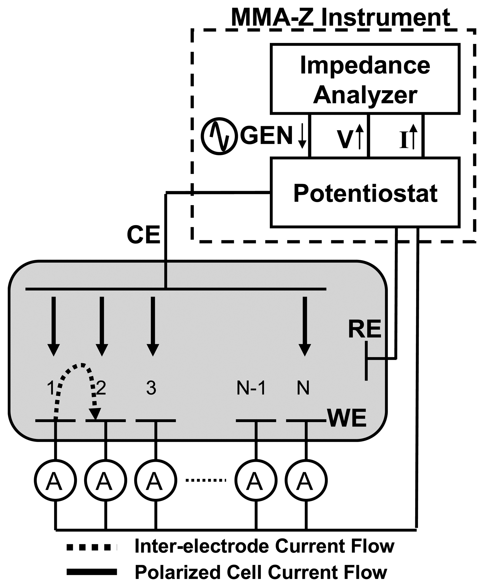
The parallel multi-channel impedance measurement approach described in Section 1.1 was implemented in the MMA. Initial tests were performed on 4 simple dummy cells: two of the dummy cells consisted of a 1 MΩ resistor, an open circuit condition reproduced a very high impedance condition, and the final dummy cell was a 1 nF capacitor. Multi-channel current and the common voltage signal were acquired at a rate of approximately 22 samples/second.
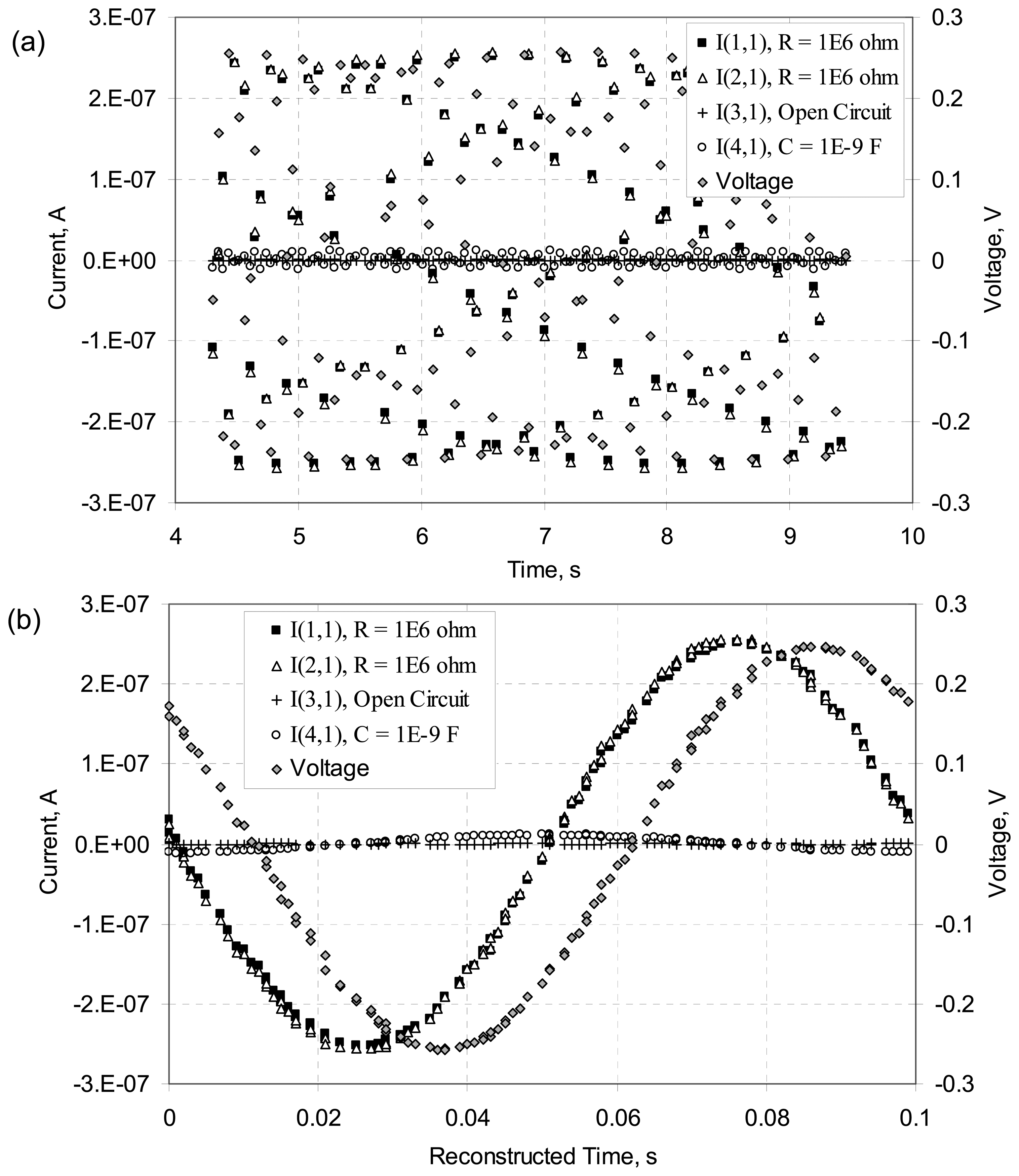
Figure 3(a) shows the original time series. As expected, for any given channel of current (I(x,y)) or the voltage data (Voltage;, there are
ca. 22 data points for every second of data acquisition. The frequency dependence of the current, if any, is not revealed in the raw time-based data, however. The raw time-based data appears as pure noise.
Figure 3(b) shows a reconstructed, single sine wave generated from the raw time-based data shown in part (a). The time base is reconstructed by subtracting a multiple of the known period of the waveform. The reconstructed time for each data point is the time since the start of the most recent waveform. The imposed 10 Hz sine wave is evident in the reconstructed data.
Note that an exact sampling rate is not necessary, and in fact could be detrimental. It is very important to know exactly when a signal was sampled, but sampling at a particular frequency is not required. That is, sampling at approximately 22 frames/second is better than measuring at exactly 22 (or 10, 20, etc.) frames/second. Consider the case in which each frame (or channel) was measured at exactly 20 times/second. For an applied AC frequency of 10 Hz, such a sampling rate would result in all of the points for a particular channel to coincide at exactly 2 locations (i.e., 2 times) within the reconstructed waveform. Such a data set would confound the subsequent FFT data analysis required for the calculation of the complex impedance. In contrast, a sample rate that is not a whole multiple of the measurement frequency causes the samples to be distributed within the reconstructed waveform.
There are two relatively simple approaches to dealing with the need for a non-perfect sampling. The first is to incorporate a small (∼ 0.01 second) random delay to the triggering of each frame. An alternative approach would use a precise sample rate that is not a multiple of the applied AC frequency. For example, sampling for 10 s at 20.01 frames/second would spread the data for any given channel over 0.1 s within the reconstructed time-base. Thus, although an exact sampling rate is not required, there is a constraint to know precisely when a signal is sampled, as demonstrated further below.
Within the reconstructed time-base of
Figure 3(b) we observe that there is an obvious phase difference between the current data for the resistors (channels I(1,1) and I(2,1)) and the capacitor (channel I(4,1)) with respect to the voltage data. That is, the current data for the resistor channels and the voltage channel data are not in-phase; ideally, current and voltage are in-phase for a purely resistive element. Likewise, current data for the channel with the capacitor element is not -90° out-of-phase with the voltage data; ideally, current and voltage are exactly out-of-phase for a purely capacitive element. The phase shift is suggestive of time skew in the data. Such time skew confounds further processing of the data for extraction of the component impedance, which is the property of interest. For each frame, all 100 currents followed by the voltage are measured in very rapid succession. Time skew in the data acquired between channels occurs because a small finite amount of time (∼ 100 μs) is required to execute each sample event.
Figure 3(b) further reveals that the time skew between the two channels with 1 MΩ resistors (I(1,1,) and I(1,2)) was small compared to the time skew between each of these channels and the voltage data; this occurs because these two current channels were measured one after the other at the start of each frame while the voltage signal was measured at the end of each frame. Fortunately, the time skew was consistent and could be accounted for.
To address the issue of time skew between channels, we determined a series of correction factors by measuring the time delay between each current sample and the voltage sample, determining the order in which each channel of current and the voltage was sampled, and assessing how the number of channels sampled influenced the time skew between samples. The MMA application software was modified to use these correction factors to automatically account for time skew between measurements in the raw time-based data. As presented below, testing with 100-element resistor arrays verified the efficacy of this approach.
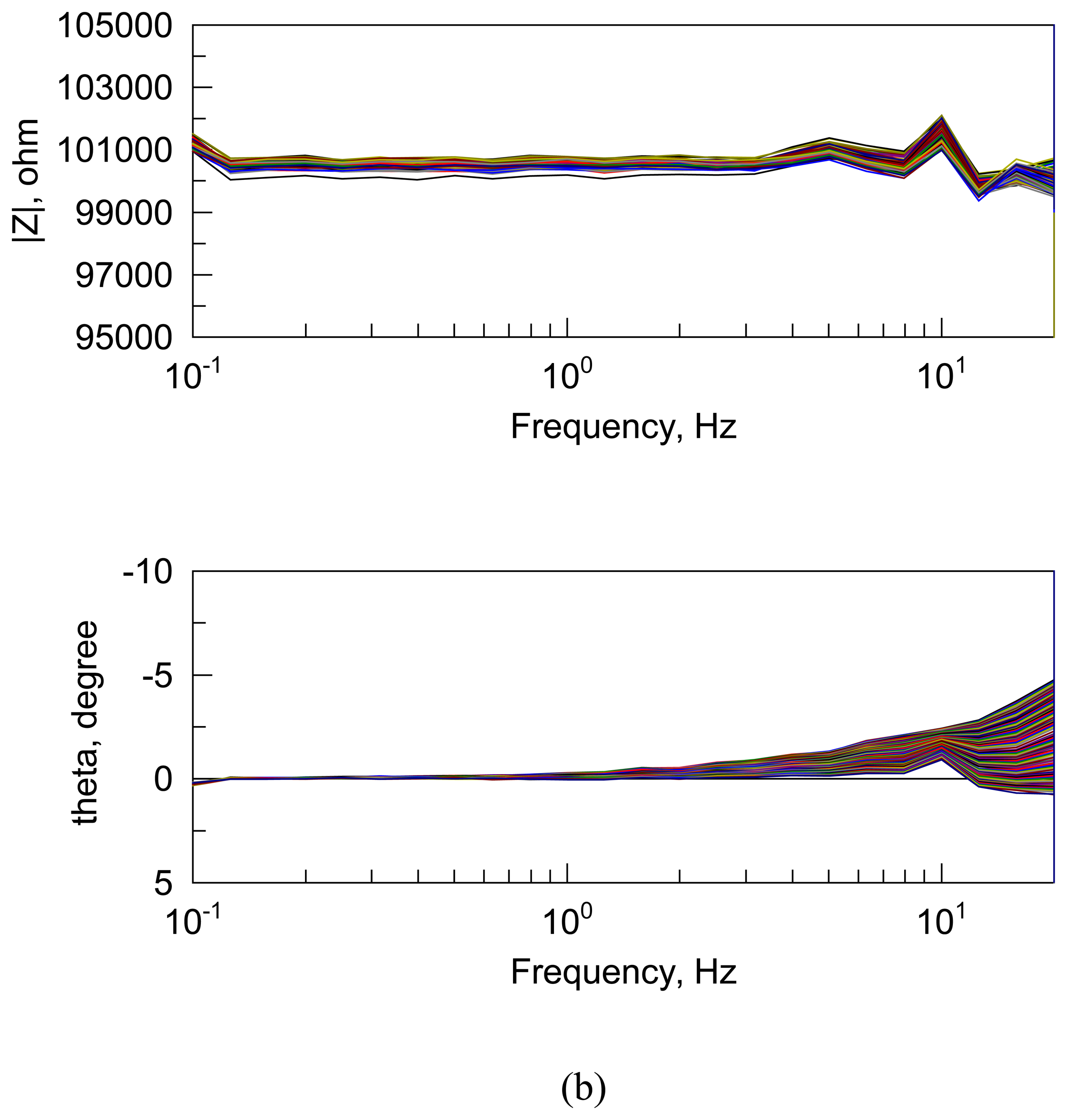
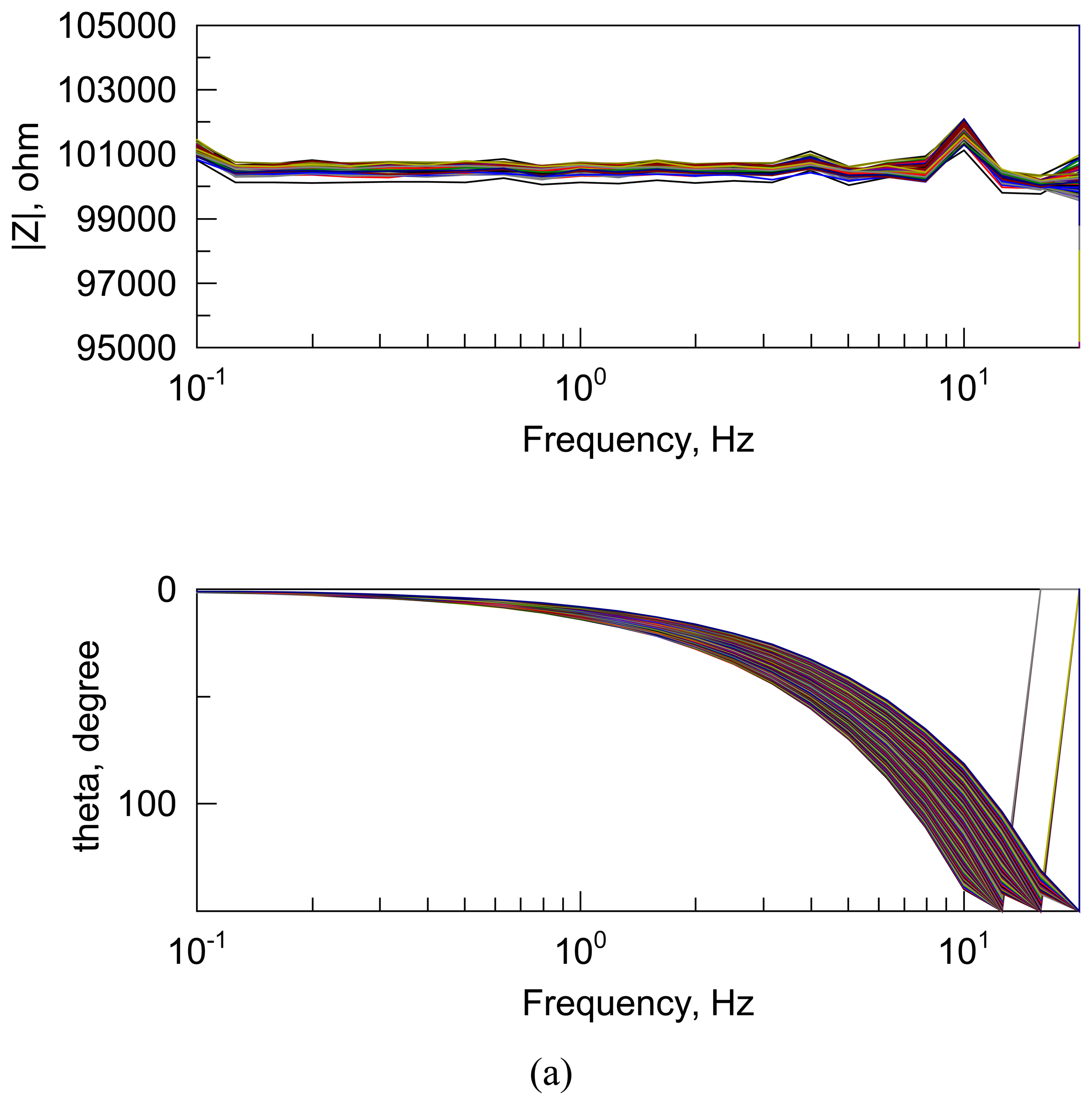
Figure 4 shows the results of a set of impedance experiments with and without the time skew correction factors applied. As described previously, time-based data was acquired in real-time at ∼ 22 frames per second and the frequency-dependence reconstructed from time-based data. Equations [
1] and [
4]-[
7] were used to calculate the impedance. The figure shows the impedance from 100 channels each connected to a 100 kΩ resistor (±1 % rated accuracy).
The effect of time skew is particularly evident by comparing the phase angle
vs. frequency graph of
Figure 4(a) and (b). These results reveal that accounting for the time skew between channels significantly improves the measurement accuracy and increases the upper frequency at which this approach may be successfully implemented. It is evident that the FFT approach to parallel low frequency impedance measurement of large arrays is feasible at frequencies less than about 20 Hz, although it should be noted that the frequency limit is hardware dependent as discussed below. At frequencies greater than 20 Hz, it is believed that time resolution and/or the accuracy of the time stamp are the dominant sources of error. The timer in the host PC is used to record the time, but there is ∼ 1 millisecond (ms) randomness between when a measurement actually starts, and when the PC “thinks” it starts. At 20 Hz (50 ms period), a 1 ms noise corresponds to about 2 % error, which is consistent with the error obtained in impedance measurements using the parallel approach at ∼ 20 Hz (see
Figure 4(b)). Future work in this area includes using a more accurate clock for the time-stamp measurement, either from the host PC/operating system or via an on-board clock, which will generate more accurate and higher resolution time-stamp information. This, along with faster data acquisition capability (more frames/second), is expected to increase the practicable upper frequency limit of the parallel impedance measurement approach.
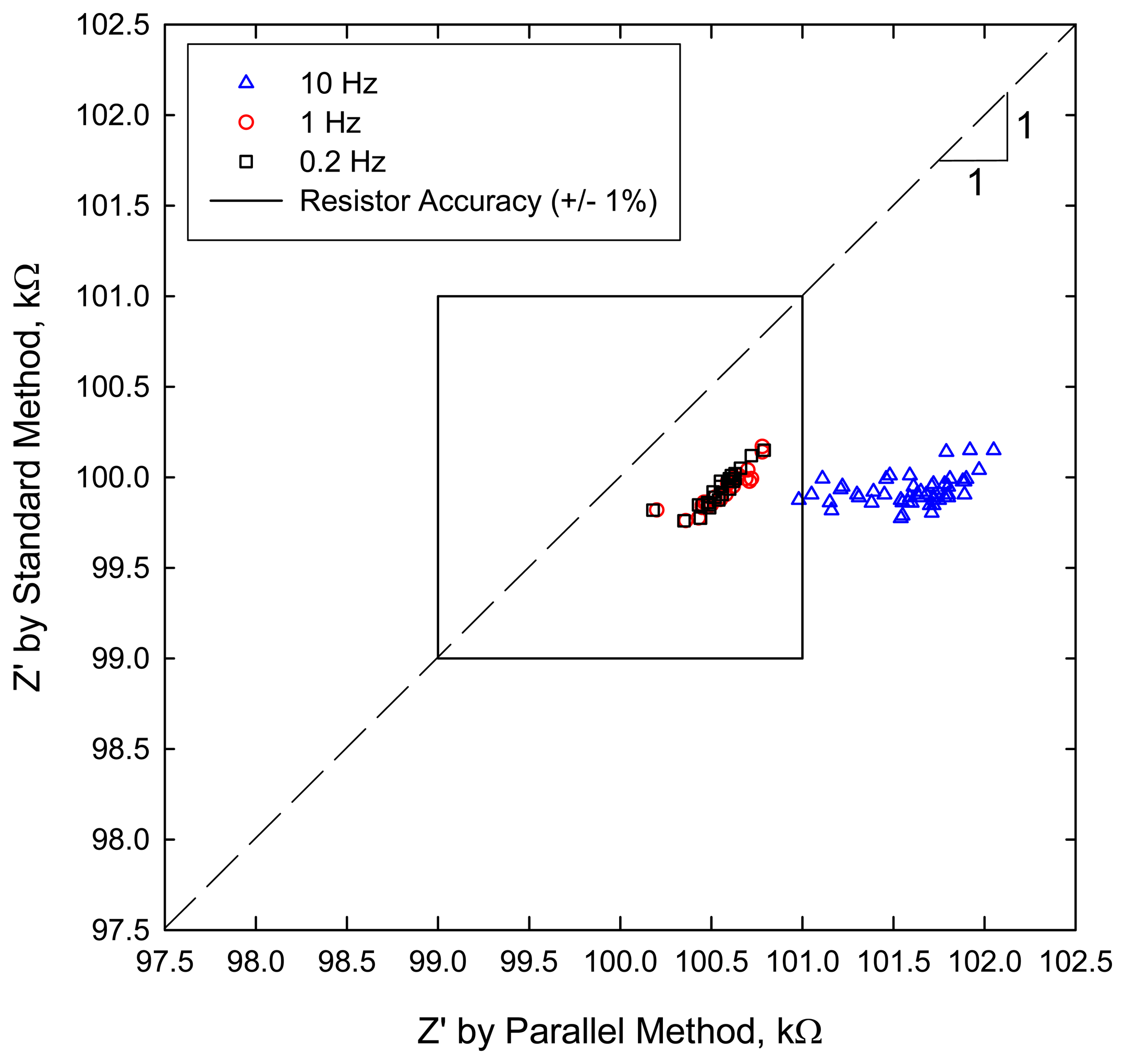
We can quantify the accuracy of the parallel method by comparing its results to that obtained with the standard method.
Table 3 summarizes statistical properties of the real component of the impedance Z′ for the parallel and standard measurement methods when measuring an array composed of ninety-eight (98) 100 kΩ resistors (±1 % rated accuracy). In addition,
Figure 5 shows the real impedance Z′ determined via the two methods where the box indicates the region of expected values based on the rated accuracy of the resistors.
Three frequencies were analyzed: 10, 1 and 0.2 Hz. Good agreement between the two methods is observed at the lowest frequencies, 0.2 and 1 Hz. In fact, close observation of the data sets at these frequencies reveals that they essentially overlap and are only slightly displaced from the 1:1 line. For these frequencies, there is less than 1 % difference between the mean of the result obtained from the parallel method and the standard method (see “%
Difference” in
Table 3).
At 10 Hz, the parallel method produced slightly greater values than the standard method. This is indicated by the larger positive %
Difference value at 10 Hz shown in
Table 3 as compared to the other frequencies as well as by the shift to the right of the 10 Hz data in
Figure 5. The discrepancy in values at 10 Hz is due to increased phase error resulting from non-optimized time skew factors and/or the effects of error in the time-stamp data. Errors due to these sources are exacerbated at higher frequency. Improvements in these areas will improve the accuracy and highest frequency at which the parallel low frequency method can be successfully applied.
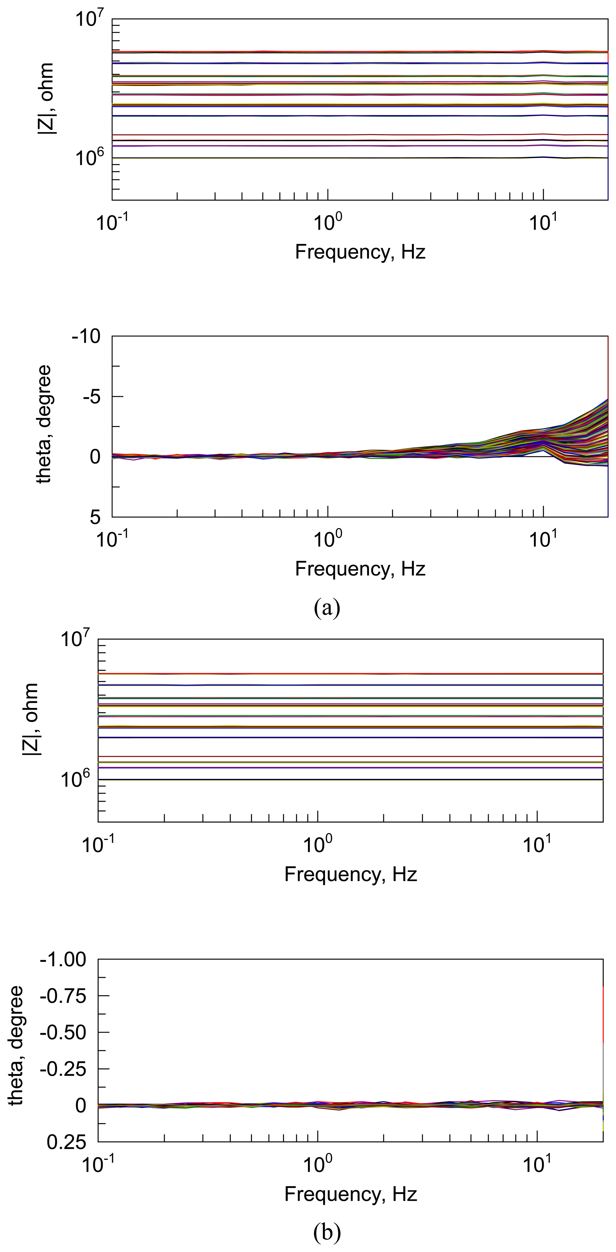
As further demonstration of the efficacy and advantage of the FFT-based parallel method for low frequency impedance measurement of electrode or sensor arrays, the impedance of an array composed of 100 resistors ranging from 1 MΩ to 50 MΩ was determined using the parallel and “standard” sequential approach. Recall that in the standard approach, at each frequency the impedance of each electrode within the array is determined before stepping to the next lower frequency. While this approach is efficient at high frequency, at low frequency the experimental time becomes significant.
Bode plots showing the impedance magnitude and phase angle (theta) as a function of frequency for both the standard sequential and parallel techniques are shown in
Figure 6. Because these figures contain a large data set (100 channels) it is not feasible to compare the results of the two methods for a given resistor value or channel. However, the results qualitatively demonstrate that the parallel method provides results that are consistent with the standard approach, in particular at frequencies less than ∼ 10 Hz for which the phase angle < 2.5° (and ideally should be 0°).
It is worth reiterating the benefit of the parallel approach to low frequency impedance spectroscopy in multi-channel systems. The following conditions were used to measure the impedance of the two types of 100-element resistor arrays presented above: 1 kHz to 0.1 Hz; 10 steps/decade; duration: 5 second per frequency for parallel method, minimum of 0.3 second or 1 cycle for standard method. For these conditions, the parallel measurement method required 7 minutes of data acquisition time whereas the standard sequential method required 120 minutes. Thus, a 17-fold reduction in experimental time was achieved by the parallel measurement method. The increase in time-efficiency of the parallel method as compared to the standard method was derived at frequencies less than about 10 Hz.
Despite the forgoing discussion, it should be recognized that ultimately one probably would not want to apply the parallel method at frequencies greater than about 10 Hz because the advantages of the parallel method, with respect to measurement time efficiency gains, are not realized at higher frequencies and because errors caused by limitations in time-based measurement accuracy are exacerbated at higher frequencies. It is better to use the standard method of impedance measurement at frequencies greater than about 10 Hz and the parallel method at frequencies less than about 10 Hz. Implementation of the optimum solution to broad frequency sweep impedance measurement of large arrays will involve the use of the standard, sequential approach at high frequencies combined with a transition to the parallel approach for the low frequency range. This hybrid or two-pronged approach to time-efficient impedance spectroscopy of large arrays is addressed in the next section.
3.2. Demonstration of efficient broadband impedance spectroscopy of large arrays
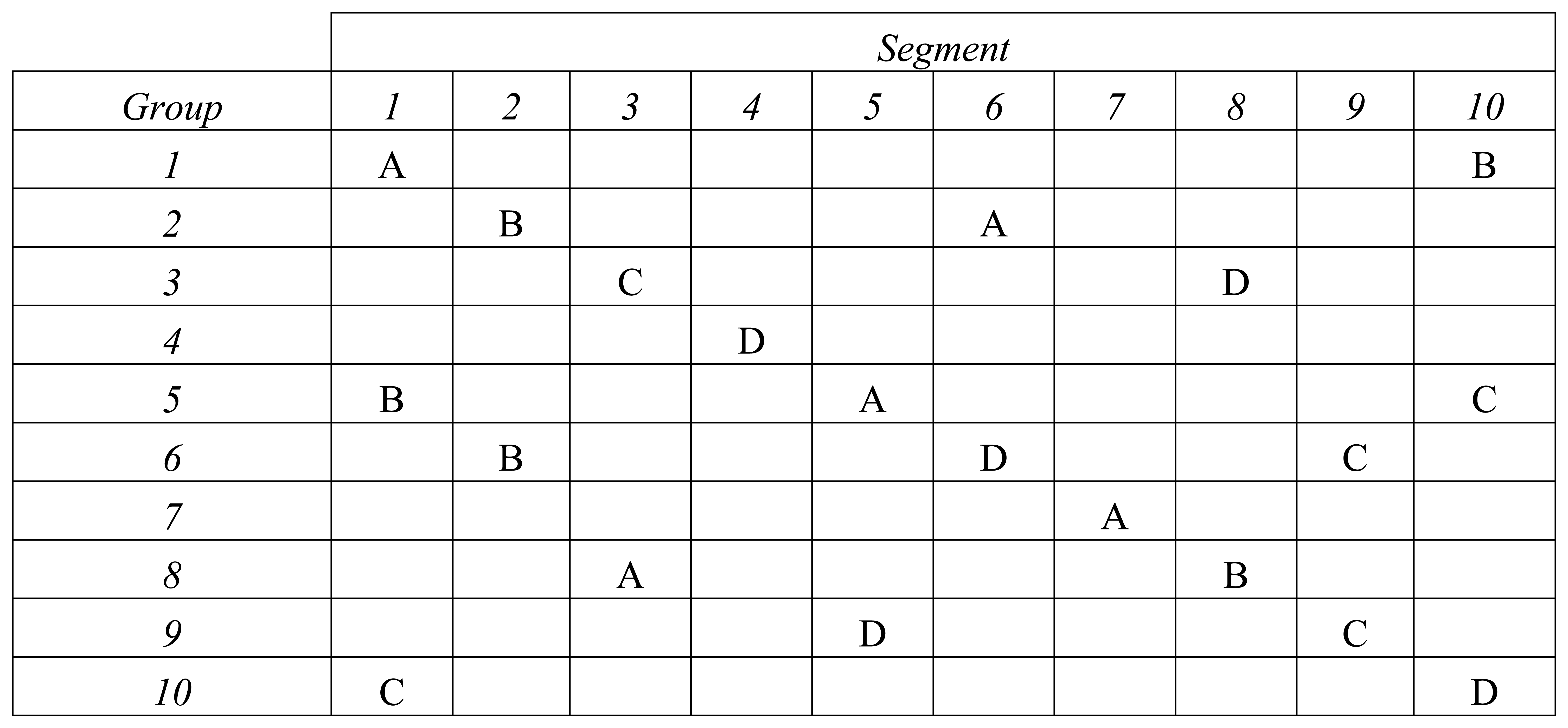
Here, we assess the performance of a multi-channel impedance analyzer with an array of dummy cells that exhibit frequency-dependent response and with impedance and reactance values consistent with typical chemiresistor sensors [
1-
4,
24,
25]. Specifically, each dummy cell was composed of a resistor (R
s) in series with a parallel resistor-capacitor element (R
p‖C
p). This specific resistor-capacitor configuration is commonly used to represent an electrochemical half-cell with a single time constant and negligible mass transport resistance [
21]. Dummy cells composed of electrical components (resistors and capacitors) have the advantage that we know
a priori the (frequency-dependent) impedance of the circuit and therefore can accurately judge the performance of the analytical instrument.
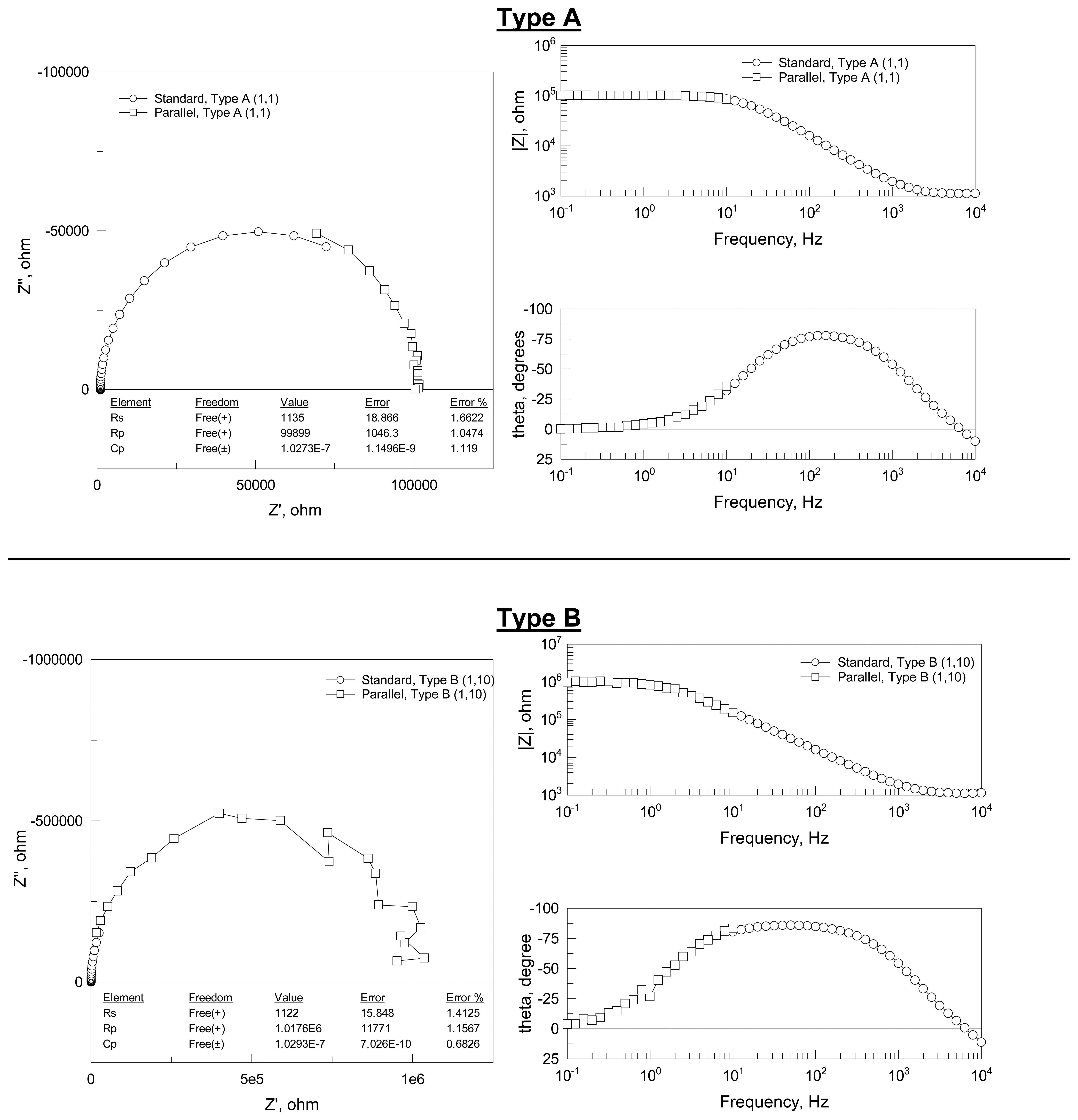
The results for the parallel low frequency impedance method are shown in
Figure 7. Because of the very large range in values of impedance exhibited by the four different types (from 1 kΩ to 11 MΩ) the results for each type of equivalent circuit are presented separately in both complex plane and Bode plot format. In addition, for each of the four different dummy circuits, an equivalent circuit model was created and its impedance modeled (
i.e., predicted) using impedance modeling software (ZView®, Scribner Associates Inc.) using nominal values for the resistors and capacitor used in the dummy cell. The predicted impedance spectra is shown as a dark green line and labeled “FitResult” in
Figure 7.
Figure 7 summarizes the low frequency impedance of the four types of equivalent circuits determined via the parallel measurement method. Within a given type of equivalent circuit the results are very reproducible. Furthermore, despite the noise observed in some of the data sets, the absolute values are correct, as evidenced by the predicted impedance spectra labeled “FitResult” in each graph. The exception are the results for the Type D dummy cell in which the measured low frequency impedance consistently exceeded the predicted value by approximately 1.1 %. The source of the discrepancy is under investigation.
Noise in the data is evident, in particular at low frequencies and for the cells with very high impedance (e.g., Type B and D) where |Z| ≥ 1 MΩ. The source of noise is due to the magnitude of the AC voltage perturbation (50 mV) and the accuracy of current measuring ZRA circuitry. The ZRAs used here were 100 μA full-scale with a resolution of 3.3 nA. At 50 mV AC and Z ∼ 1 MΩ, the current was no more than ∼ 50 nA and generally much less than this value. Higher impedance results in even lower current signal. Such small currents approach the bit-resolution of the instrument and thus increase the noise in the data. The remedy to this problem is to match the current measurement circuitry and/or the magnitude of the AC voltage perturbation to the impedance to be measured. It should be noted that using a larger AC perturbation than used here would significantly reduce the noise (but may not be practical for real systems that exhibit non-linear response).
The array analyzers' ZRA circuitry has a limited number of ranges which it can use to optimize measurement of the current, thus limiting the measurable range of impedance to ∼ 5 to 6. As such there is an inherent challenge when one type of ZRA circuit is called upon to measure the impedance over 8 orders of magnitude. Fortunately, if the impedance range of a given sensor (or electrode system under study) is known, the current measuring circuitry and possibly the AC voltage perturbation can be selected for optimum measurement accuracy and resolution over the full range of the system response.
As indicated in the experimental section, two types of impedance experiments were conducted: the standard sequential measurement approach and the parallel low frequency approach described in detail above. The results of the equivalent circuit dummy cell impedance testing using the parallel approach are presented above. Next, we merged the results of the standard method covering the high frequency range (10 kHz to 10 Hz) with the results of the parallel method restricted to the low frequency range (10 Hz to 0.1 Hz) to demonstrate the efficacy of efficiently obtaining broadband impedance spectra.
Table 4 compares the total measurement time using the standard sequential approach over the whole frequency range (10 kHz to 0.1 Hz)
vs. the combined standard + parallel approach over the indicated frequency ranges. As indicated there is an 11-fold reduction in measurement time when using the combined standard + parallel measurement approach in comparison to the standard sequential method alone. Note that measuring to lower frequencies would exponentially increase the time for the standard method but only linearly increase the time for the parallel method. Hence, even greater benefits in measurement time efficiencies are obtained at lower frequencies through implementation of the parallel method.
Figure 8 summarizes the impedance spectra obtained using the combined measurement approach. The data indicate that it is feasible to merge the results from the two different measurement approaches to produce complete, broadband impedance spectra of large electrode arrays in a time-efficient manner.
The results of equivalent circuit fitting of the combined standard + parallel experimental impedance data provide an indication of the accuracy of the measurement. The results of the fit along with the nominal dummy cell resistor and capacitor values for one of each of the four different types of circuit are shown in
Table 5. In general, the fit results were very close to the nominal values of the component used to build the dummy cell. In all cases, the difference between the predicted value of the circuit capacitance (C
p) and the nominal value was 3 % or better for 3 of the 4 circuits. The exception was for type D which had an error ∼ 7 %. Likewise, the predicted value of the parallel resistor (R
p) was within 2 to 10 % of the nominal value.
There was, however, a > 10 % error in the fitted value of the 1 kΩ series resistor (Rs) used in the Type A and B dummy cells, which was observed in other experiments as well, and only occurs when measuring a dummy cell containing a parallel resistor-capacitor (Rp‖Cp) element. That is, this error is not evident when measuring a resistor alone. Neither was this error observed when Rs ≫ 1 kΩ, e.g., type C and D dummy cells. The source of this error is uncertain.
The results demonstrate that, in general, the large-channel count array analyzer used here was capable of accurately measuring the impedance of dummy cells designed to simulate typical chemiresistor (and other) sensors [
1-
4,
24,
25]. Equivalent circuit fit results of experimental data acquired using the combined standard + parallel approach resulted in predicted values of the circuit components that were very close to the nominal value used to fabricate the dummy cell.


