1. Introduction
Wireless sensor networks (WSNs) can implement various complicated tasks in the sensing field via a large number of smart wireless sensor nodes which have sensing, storage, processing and communication capabilities. All the wireless sensor nodes work collaboratively to leverage their individual efforts for the entire application. Since battery-powered wireless sensor nodes are greatly constrained with regards to energy supply, energy efficiency becomes a critical problem in WSNs. As an essential requirement, sensing coverage has been investigated in a few literature reports [
1,
2]. The coverage problem is defined from several points of view, including deterministic, statistical, worst and best case in [
3]. In particular, efficient network deployment considering coverage as well as connectivity is discussed in [
4,
5]. Target tracking is a typical application for WSNs and poses a great challenge to achieve both high reliability and long lifetime [
6]. For WSNs which implement target tracking applications, the efficiency of energy usage should be taken into account in the deployment. Generally, wireless communication spends much more energy than sensing and computation, so it should be the primary consideration [
7]. In addition, the potential processing capability of multiple wireless sensor nodes may contribute to better optimization performance [
8].
Due to the above-mentioned requirements of deployment in WSNs, we propose distributed particle swarm optimization and simulated annealing (DPSOSA) for energy-efficient coverage. This method takes the energy consumption of target tracking into account to optimize the energy efficiency of WSN coverage with distributed computing. Sensing coverage and energy consumption models for WSNs are introduced first. The purpose of optimization is to find the best deployment of mobile wireless sensor nodes so that the sensing coverage requirement is satisfied and communication energy consumption can be minimized. Then the grid exclusion algorithm is exploited to calculate the coverage rate of specific network deployment, which has minimized computational cost and scalable granularity. We adopt Dijkstra's algorithm to search the lowest cost paths for data collection, which will be regarded as packet transmission paths in target tracking applications. The sensing coverage rate and total energy consumption of data collection are defined as coverage and energy metrics, respectively. The DPSOSA algorithm is then employed to optimize the communication energy consumption under a given sensing coverage requirement. It is executed over a number of nodes, in which the particle swarm optimization (PSO) procedure is aided by the optimization results of simulated annealing (SA) for the global optimal solution. In DPSOSA, a number of particles are given a better view to search for better solutions in their vicinity, by which the PSO procedure can be corrected. Meanwhile, as multiple particles need to be optimized, the optimization task is assigned among wireless sensor nodes to boost up the computational capability. With simulations of deployment optimization and target tracking, the energy efficiency of the proposed distributed optimization algorithm is verified.
The rest of this paper is organized as follows: section 2 formulates the energy-efficient coverage problem with stationary and mobile wireless sensor nodes in WSNs, where the sensing coverage and energy consumption models are presented. In Section 3, two important metrics, coverage and energy, are defined for network deployment evaluation according to the fundamental model, where the grid exclusion and Dijkstra' algorithm are introduced. Then Section 4 presents the DPSOSA algorithm for energy-efficient coverage in WSNs. In Section 5, we simulate the deployment optimization algorithm for target tracking application and analyze energy-efficiency of WSNs. We conclude the paper in Section 6.
2. Preliminaries
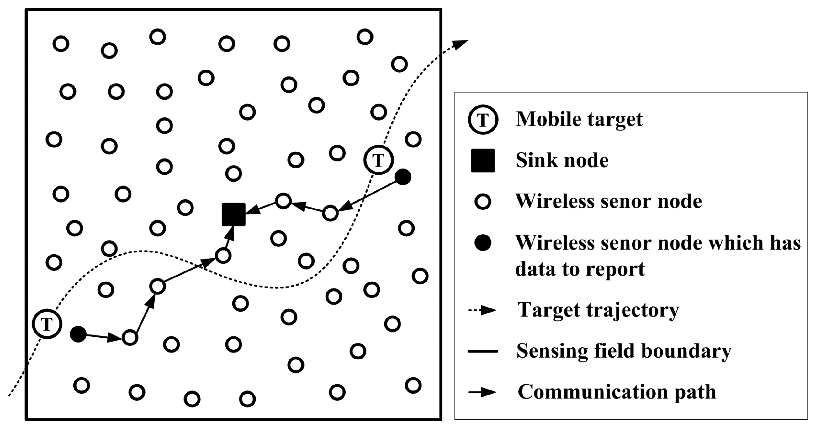
We assume a WSN composed of two types of wireless sensor nodes: stationary and mobile nodes. In the sensing field, the stationary nodes are deployed randomly, while the mobile ones can adjust their positions adaptively against the environment. With the mobile nodes located at their proper positions, WSN can implement target tracking applications. As shown in
Figure 1, wireless sensor nodes which are close to the mobile target trajectory may acquire data. A sink node is located in the centre of sensing field, to which the observations will be forwarded hop by hop [
9,
10]. It is assumed that the positions of nodes can be obtained by global positioning system (GPS) [
11]. In this section, we will describe the sensing coverage model for reliability detection. Considering the energy efficiency problem, energy consumption model of communication will be discussed.
2.1. Sensing coverage model
Each wireless sensor node integrates three radar sensors with the same sensing radius
R, oriented at 120° intervals. Azimuth coverage of radar sensor is −60° ~ +60° [
12]. For each wireless sensor node, it is assumed that the strength of received detection signal varies exponentially with the distance from the target. If the coordinates of wireless sensor node
i and a target are (
xi,
yi) and (
xtarget,
ytarget), respectively, the received signal strength reflected off the target is:
where
G0 is a constant which denotes the strength of emission signal,
β is the attenuation constant. And
dtarget,i is the Euclidean distance between the target and sensor:
According to the sensitivity and reliability of sensor, we can define a threshold of received signal strength
Gth, and calculate the detection reliability as:
where
r0 is the reliability of sensor when the received signal strength exceeds
Gth, 0 <
r0<1. Thus, wireless sensor node
i can physically cover a plate area with radius
Ra, where the centre locates at (
xi,
yi). The sensing radius
Ra can be calculated as:
Considering the inherent redundancy of WSNs, we discuss the
k-coverage problem, that is, certain area is covered by
k or more wireless sensor nodes at the same instant. In this case, synthesis detection reliability of the area is at least:
Therefore, we can acquire high synthesis detection reliability even though the detection reliability of individual wireless sensor node is limited.
2.2. Energy consumption model
During target tracking, wireless sensor nodes have the functions of data acquisition, processing and reporting. The related sensing, computation and communication operations will lead to energy depletion. Out of all the energy consumption sources in WSNs, wireless communication is the largest portion. Thereby, it is the main one taken into account here. As radio signal attenuation in the air is related with the propagation distance, we adopt the free space propagation model [
13], which is expressed as:
where
Lp is the path loss,
λs is the wavelength of signal, and
di,j is the propagation distance. If radio signal propagates between wireless sensor node
i and
j, which are located at (
xi,
yi) and (
xj,
yj), the corresponding propagation distance can be calculated as:
Accordingly, a model of wireless communication is assumed to analyze energy consumption of communication. Here, the power consumption of data transmission between wireless sensor node
i and
j is calculated as [
14]:
where
rd denotes the data rate,
α1 denotes the electronics energy expended in transmitting one bit of data,
α2>
0 is a constant related to the radio energy. Given the transmission tasks through the network, the energy consumption feature of WSNs can be obtained.
3. Evaluation Metrics of Energy-efficient Coverage
To achieve reliable detection and energy conservation in target tracking application, WSNs should apply an energy-efficient coverage scheme. Coverage and energy performance is concerned in potential mobile node deployment. For specified detection reliability, sensing area needs to be covered by certain number of wireless sensor nodes. The area which can satisfy this reliability requirement in the whole sensing field can reflect the coverage performance. On the other hand, data packet transmission from wireless sensor nodes to the sink node results in energy consumption. An energy-efficient communication framework can be established by the lowest cost paths. This framework indicates the lowest energy consumption level which can be provided by different deployment of WSNs.
It is assumed that there are n stationary nodes and m mobile nodes in a L × L square sensing field. The coordinates of sink node are (L/2, L/2). In a possible network deployment, the coordinates of all wireless sensor nodes (xi,yi)(i=1,2,..,n+m) can be obtained, where the indices of the stationary and mobile nodes are (i=1,2,..,n) and (i=n+1,n+2,..,n+m), respectively. Accordingly, coverage and energy metrics and related algorithms will be presented to evaluate the network deployment in this section.
3.1. Coverage metrics
Typically, certain detection reliability
Rreq is required for specific target tracking application. Based on
Equation (5), the required number of wireless sensor nodes, which can detect the target with reliability
r0 at the same time, can be calculated as:
The area which is covered by kreq or more wireless sensor nodes is regarded as the reliable detection area. To provide integrated and continuous detection of targets in the sensing field, the reliable detection area should be as large as possible. Therefore, we define the proportion of reliable detection area in the whole sensing field as the coverage metric.
As discussed in Section 2.1, each wireless sensor node covers a plate area with radius Ra. Due to the irregular network deployment, the coverage state problem is too complicated for geometric analysis. Thus, we exploit a numerical method, the grid exclusion algorithm, to extract the coverage state information. The pseudo-code for grid exclusion algorithm is outlined in Algorithm 1.
Algorithm 1
1. Initialization
Divide the square sensing field into lxl uniform grids. Each grid is a (L/l)×(L/l) square area.
Simplify the grids into points, then each grid can be denoted by its centre point. The coordinates of points are:
Initialize the coverage state matrix {cov(i,j)}:
Set the number of reliable detection point num = 0 and set the number of unreliable detection points nr=0.
2. Coverage state for stationary nodes on the whole sensing field
Check the detection reliability point by point.
| For xg = L/2l,3L/2l,…,(2l-1)L/2l |
| For yg = L/2l,3L/2l,…,(2l-1)L/2l |
| This point is related to the element cov(ig,jg) of the coverage state matrix: |
|
| Check whether stationary node i covers this point. |
| For i= 1, 2,…, n |
| Calculate the distance between stationary node i and the point: |
|
| Update the coverage state matrix as: |
|
| End |
| If cov(ig,jg) > kreq |
| Update the number of reliable detection point: |
|
| Else |
| Record the unreliable detection point: |
|
| End |
| End |
| End |
The coverage state matrix of stationary nodes is obtained.
3.2. Energy metrics
During target tracking in WSNs, wireless sensor nodes spend significant energy reporting their observations. With the model presented in Section 2.2, we analyze the energy consumption of wireless communication.
According to
Equation (8), the wireless sensor nodes which are far away from the sink node would spend too much energy when their data packets are transmitted directly. These nodes may find a number of other nodes for data forwarding and such a multi-hop manner will potentially conserve energy. Thus, the lowest cost path to sink node should be found for each wireless sensor node.
Here, Dijkstra's algorithm is introduced to solve this lowest path problem, which can accomplish breadth-first path search between one single destination vertex and all the other vertexes on the connected graph [
15,
16]. Since any vertex that has shorter path to the destination vertex is traversed, the optimal solution can always be found.
For any given WSN deployment, the sink node is regarded as the destination vertex and denoted by
u0, while wireless sensor nodes are taken as all the other vertexes and denoted by
U={
u1,
u2,…,
un+m}. The edge weight between vertex
ui and
uj is defined according to
Equations (7) and
(8):
Then the pseudo-code for the lowest cost path search is outlined in Algorithm 2.
Algorithm 2
1. Initialization
Adopt variable Di to represents estimate of the lowest cost from ui to u0. It converges to the real value after iterations. Initialize the connected graph as:
The set of vertexes which have found the lowest cost paths is denoted by Q, set Q=Ø.
2. Iteration
| While Q ≠ U |
| Find the next vertex with the lowest cost path to u0. |
| For any vertex ui ∉ Q |
| If Di satisfies: |
|
| The lowest cost path from vertex ui to u0 is found. |
| Update Q: |
|
| Record the vertex ui, set i0=i. |
| End |
| End |
| For any vertex uj ∉ Q |
| Update Dj: |
|
| End |
| End |
After iteration, Di denotes transmission energy consumption per bit from vertex ui to u0 adopting the lowest cost path, where i = 1, 2,…, n+m.
Thus, the lowest cost paths from all wireless sensor nodes to sink node are available, which form an energy-efficient communication framework. This framework reflects the lowest energy consumption level which can be provide by the given network deployment. Since each wireless sensor node has the opportunity to detect a target and report its data, we can evaluate the energy consumption by the total cost of all the reporting paths. Therefore, the energy metric
E of network deployment is calculated as:
Generally, different deployment of mobile nodes corresponds to different energy metric values. The proposed coverage and energy metric will be used to evaluate different network deployment in the optimization algorithm.
4. Distributed Optimization Algorithm for Energy-efficient Coverage
When WSNs are initially organized, proper deployment of mobile nodes is desirable to achieve energy-efficient coverage. Also, the environment may cause changes in WSNs, such as the appearance of node failures. Therefore, position adjusting of mobile nodes is necessary for resource re-allocation. With the proposed coverage and energy metrics, deployment optimization should be implemented to provide adaptability for WSNs in these cases. Then, the optimization results are broadcasted over the network so that WSNs can be self-organized.
Following the previous assumption, there are n stationary nodes and m mobile nodes available in the deployment problem. The coordinates of mobile nodes are taken as non-integral input vectors for optimization. As described in Section 3.1, certain coverage ratio C0, namely the optimized coverage metric, is demanded under the detection reliability requirement. Thus, the objective of optimization is to decrease the energy consumption level of WSNs in target tracking applications under the condition that the required coverage metric is satisfied.
Kennedy
et al. developed particle swarm optimization in 1995 based on the analogy of swarms of birds and fish schools. PSO is an efficient optimization tool for solving combinatorial optimization and dynamic optimization problems in multi-dimensional space, which implements fast convergence and good robustness [
17]. Here, it is considered as a deployment optimization algorithm in WSNs. Like other evolutionary algorithms, PSO uses a fitness function as criterion to evolve the behavior of the solution population. In the algorithm, potential solutions, namely particles, fly through the search space. Each particle keeps track of the best position it has achieved so far, which represents a particle experiment. Another kind of experiment is the best position which has been achieved by the companion of particle so far. The particle velocity is constantly adjusted according to the two kinds of experiences.
PSO has a strong ability for finding the most optimal result. However, it has a disadvantage in local minima. Thus, simulated annealing [
18] which has a strong ability for finding the local optimal result is introduced to avoid the problem of local minima. SA mainly consists of the repeating of two steps: a generation mechanism and an acceptance criterion. It starts off at an initial random state with a high temperature, and then a sequence of iterations is generated. A perturbation mechanism transforms the current state into a next state selected from the neighborhood of the current state. If this neighboring state has better fitness, the neighboring state is accepted as the current state. If this neighboring state has worse fitness, the neighboring state is accepted with a certain probability determined by the acceptance criterion [
19]. After sufficient times of acceptance, the temperature is decreased. This process is repeated until the final temperature is reached.
We propose distributed particle swarm optimization and simulated annealing here. SA is applied on the global best position of PSO. Then the vicinity of the global best position is searched to obtain a local optimal result. Thereby, the procedure of PSO is corrected by the result. In the same way, the best position achieved by individual particle can be corrected by SA. Since SA maintains only one solution, this extended optimization tasks can be assigned simply to a number of wireless sensor nodes utilizing the distributed computing capacity of WSNs. The pseudo-code for DPSOSA is outlined in Algorithm 3.
Algorithm 3
The sink node performs main part of the algorithm.
1. Initialization
The population of particles is set as pop.
| For i = 1, 2,…, pop |
| For particle i, Xi represents the current position, where the elements present the coordinates of all mobile nodes: |
|
| Vi represents the current velocity it has achieved so far: |
|
| Pi represents the best position it has achieved so far: |
|
| Initialize Xi as a random position Xi (1) in the search space. |
| Initialize Vi as a random velocity Vi (1). |
| Set the initial Pi as: |
|
| End |
According to the purpose of energy-efficient coverage in WSN, the minimization objective function
f(X) is defined for the position
X of any given particle as:
where
E and
C are the metrics defined in Section 3.1 and 3.2 respectively.
E0 is a constant which denotes the upper bound of energy metric, while
C0 is the demanded coverage ratio.
ρ is a constant for balancing the two metrics.
2. PSO iterations
| For t = 1, 2,…, PSO_ITER |
| The global best position of particle is calculated as: |
|
| For i = 1, 2,…, pop |
| The velocity of particle is updated as: |
|
Γ
1={
r1j} and Γ
2={
r2j} are two separate random sequences, where
j = 1, 2,…, 2
m,
c1 and
c2 are acceleration constants, representing the weight of acceleration terms that pull each particle toward the local best position and global best position and
η(t) is the inertia weight for balancing the global and local search ability. It is defined as:
|
| The position of particle is updated as: |
|
| The best position of particle is calculated as: |
|
| End |
The sink node sorts Pi(t+1) by their fitness. Select the best SA_NUM positions {Pis|i = 1, 2,…, SA-NUM}, which are to be optimized with SA. The optimization of global best position will be performed by the sink node, while SA_NUM –1 wireless sensor nodes are randomly selected to optimize the other positions.
The sink node transmits each particle to the related node. Then sink node and these nodes perform parallel SA optimization.
| For i = 1, 2,…, SA-NUM |
| Perform SA iterations taking the initial state as: |
|
| Set an initial temperature T. |
| For k = 1, 2,…, SA-ITER |
| The cooling condition is that the best state remains unchanged for K times. |
| While the cooling condition is not satisfied |
| Use a perturbation mechanism to generate a new state A': |
|
| where rand_norm is a normally distributed random number, Δ = {δj|j = 1, 2,…, 2m} and Δ = {δj | j = 1,2, ⋯, 2m} and δj is defined with a random integer j0 in [1, 2m]: |
|
| The decrease of fitness is: |
|
| Check whether the new state should be accepted according to Metropolis criteria. |
| If df < 0 |
| Accept the new state: A = A'. |
| Else if e−df/(γT) > rand, where γ is Boltzmann constant and rand is a random number in [0,1] |
| Accept the new state: A = A'. |
| Else |
| The new state A' cannot be accepted. |
| End |
| End |
| Cool down with a parameter λ: |
|
| End |
| End |
| If any result is better the initial state, the wireless sensor node sends it back to the sink node, where the former position will be replaced. |
| End |
Finally, the global best position presents the optimized deployment of WSN.
In PSOSA, the sink node performs PSO_ITER iterations of PSO, where the inertia weight η(t) linearly decreases through the course of the run. A large inertia weight facilitates a global search while a small inertia weight facilitates a local search. Accordingly, the optimization process can converge to the neighborhood of the global optimal solution smoothly at the prophase and converge to the global optimal solution quickly at the anaphase. SA_NUM local best positions are optimized by SA on the sink node and SA_NUM –1 other wireless sensor nodes. After SA_ITER iterations of SA, the optimized results are utilized to correct the former positions. In this way, the algorithms have good potential to obtain the optimal deployment of WSNs.
5. Simulation Experiments
In this section, we will analyze the efficiency of DPSOSA algorithm with simulation experiments. The simulation environment will be specified. Then the simulation and comparison of algorithms will be given. Finally, the network simulations will be present for target tracking application.
5.1. Simulation environment
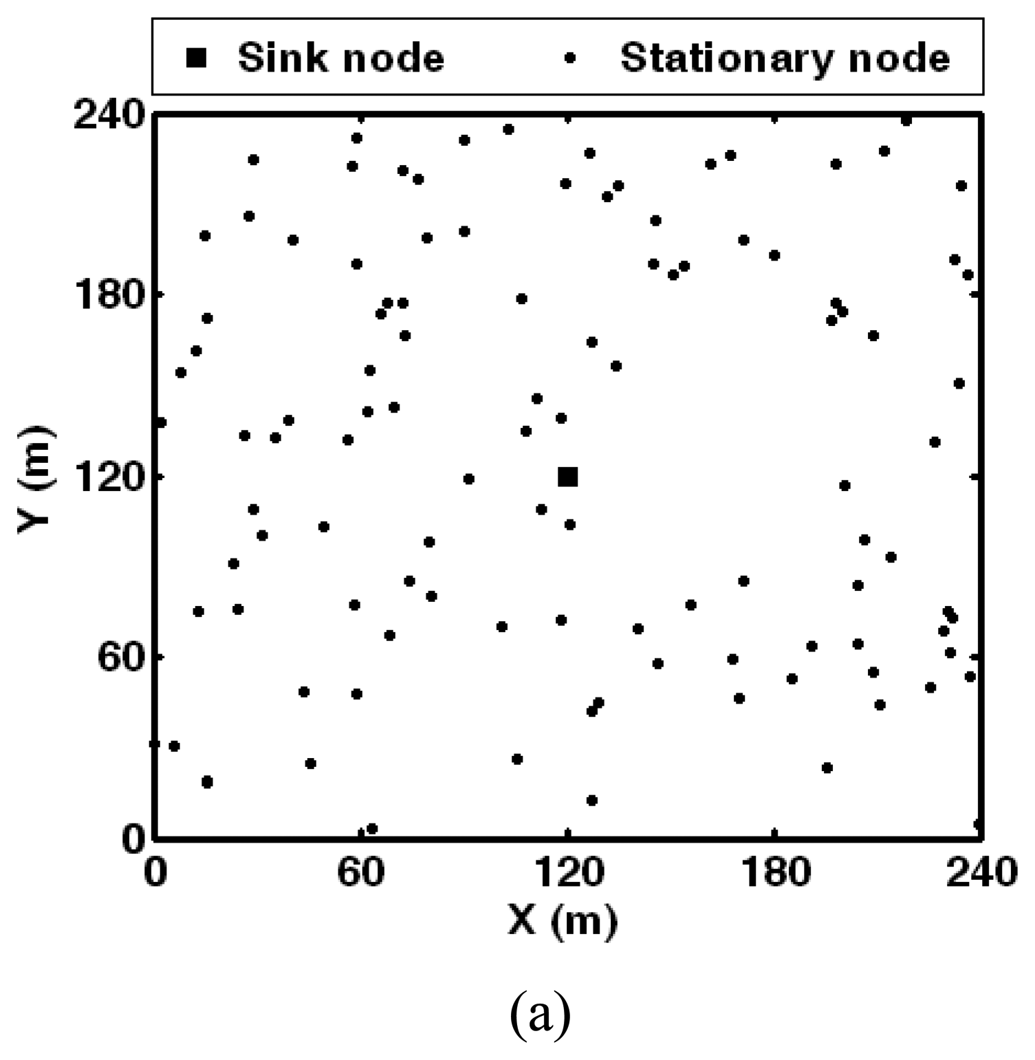
The fundamental parameters of WSN are presented in
Table 1. The stationary nodes are placed randomly in the square sensing field as shown in
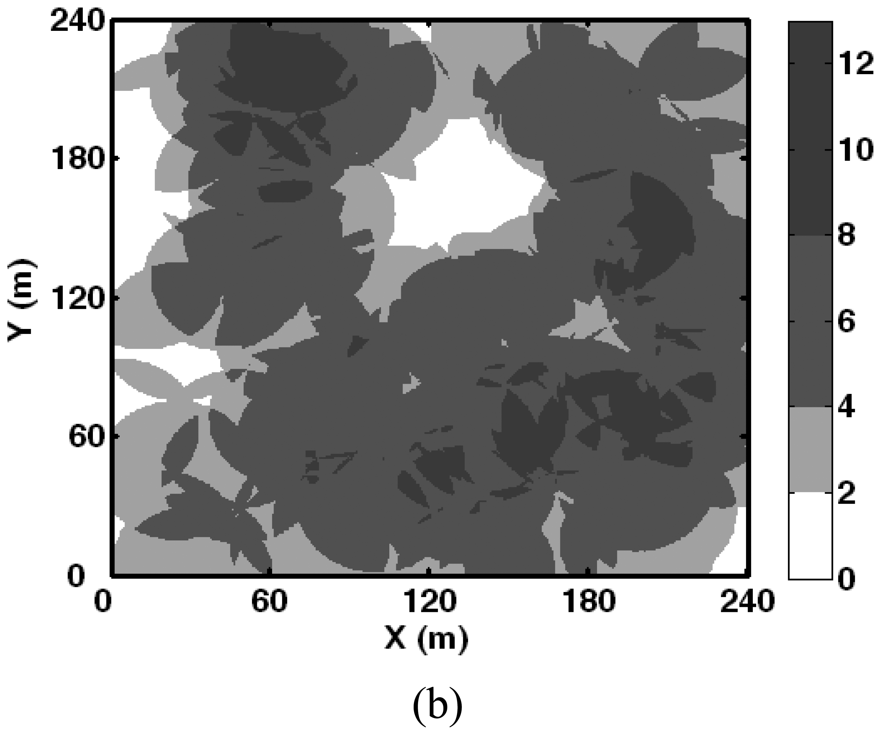
Figure 2(a). With the specified sensing radius of wireless sensor node, we can calculate the initial coverage state of stationary nodes according to Section 3.1.
Figure 2(b) shows the initial coverage state, and the area with darker grey levels means that there is coverage by more nodes.
In the energy consumption model, we set
α1 = 50
nJ/
bit and
α2 = 100
pJ/
bit/
m2. When we calculate the coverage metric, the sensing field is divided into 100 × 100 uniform grids. Accordingly, the initial coverage metric of
k-coverage area is presented in
Table 2, where
k changes from 1 to 6. As more covering nodes are required to satisfy the reliability, the initial coverage metric turns lower rapidly. Based on
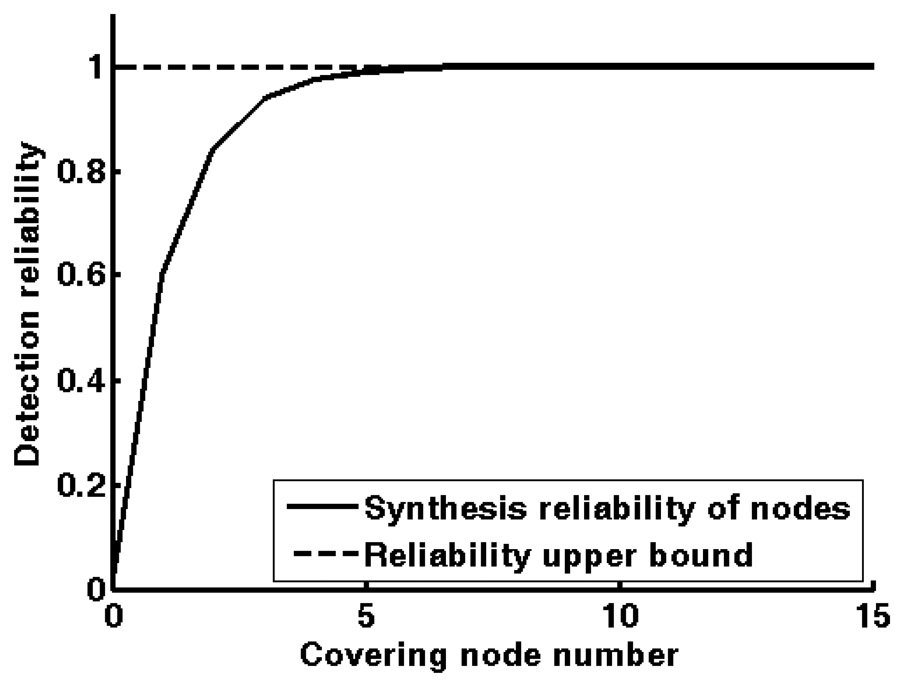
Equation (5),
Figure 3 illustrates the detection reliability with different covering node number. The detection reliability grows exponentially and exceeds 0.99 when the covering node number is 6.
In the DPSOSA algorithm, the particle number pop is set as 30, the acceleration constants c1=c2=1, and the PSO iteration number PSO_ITER is specified as 40. During each SA optimization, we set initial temperature T as 0.0001 according to the fitness function. Parameter K is 4 in the cooling condition, while the cooling parameter λ is 0.6. Besides, Boltzmann constant γ = 1, and the PSO iteration number SA_ITER is specified as 5.
Target tracking application of the optimized WSN will be simulated on a modeling platform, Opnet Modeler, which is developed for communication network and distribution system. It is assumed that the sampling period of WSN is 0.5 s. Without loss of generality, a mobile target moves randomly in the sensing area for 120 s. Wireless channel model is bpsk, the free space propagation model is utilized and data rate is 1 Mbps.
5.2. Simulations of deployment optimization
With the stated simulation environment, the DPSOSA algorithm can be adopted to achieve energy-efficient coverage. First, we should define the coverage requirement, which is given by two parameters, detection reliability
Rreq and coverage ratio
C0. Considering the initial coverage state, we discuss two kind of coverage requirement to analyze the performance of algorithm against different conditions: (1)
Rreq = 0.8,
C0 = 95%; (2)
Rreq = 0.9,
C0 = 95%. The required covering node numbers
kreq are 2 and 3 respectively. According to
Table 2, the latter coverage requirement is much stricter than the former one.
Second, the constant
E0 which denotes the upper bound of energy metric should be specified for the fitness calculation. Here, we search the lowest cost paths of the station nodes without any mobile node. Assume the related path cost is {
Dsi |
i = 1, 2,…,
n}, then
E0 is defined as:
In this case,
E0 is 7.26 × 10
−5J/
bit, and
ρ is set as 10
5.
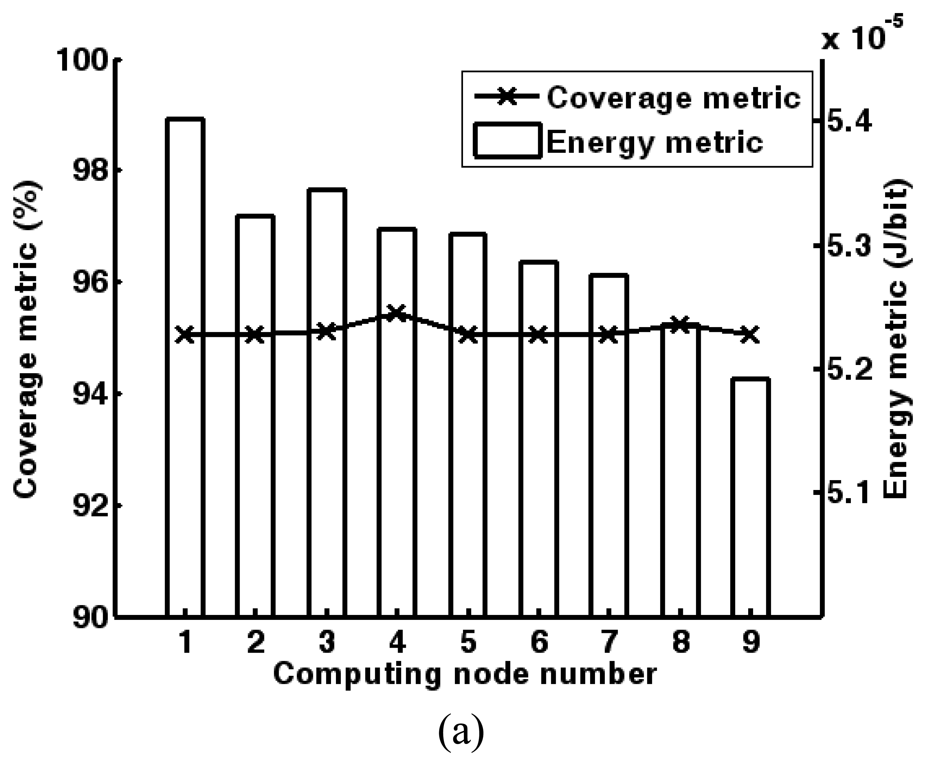
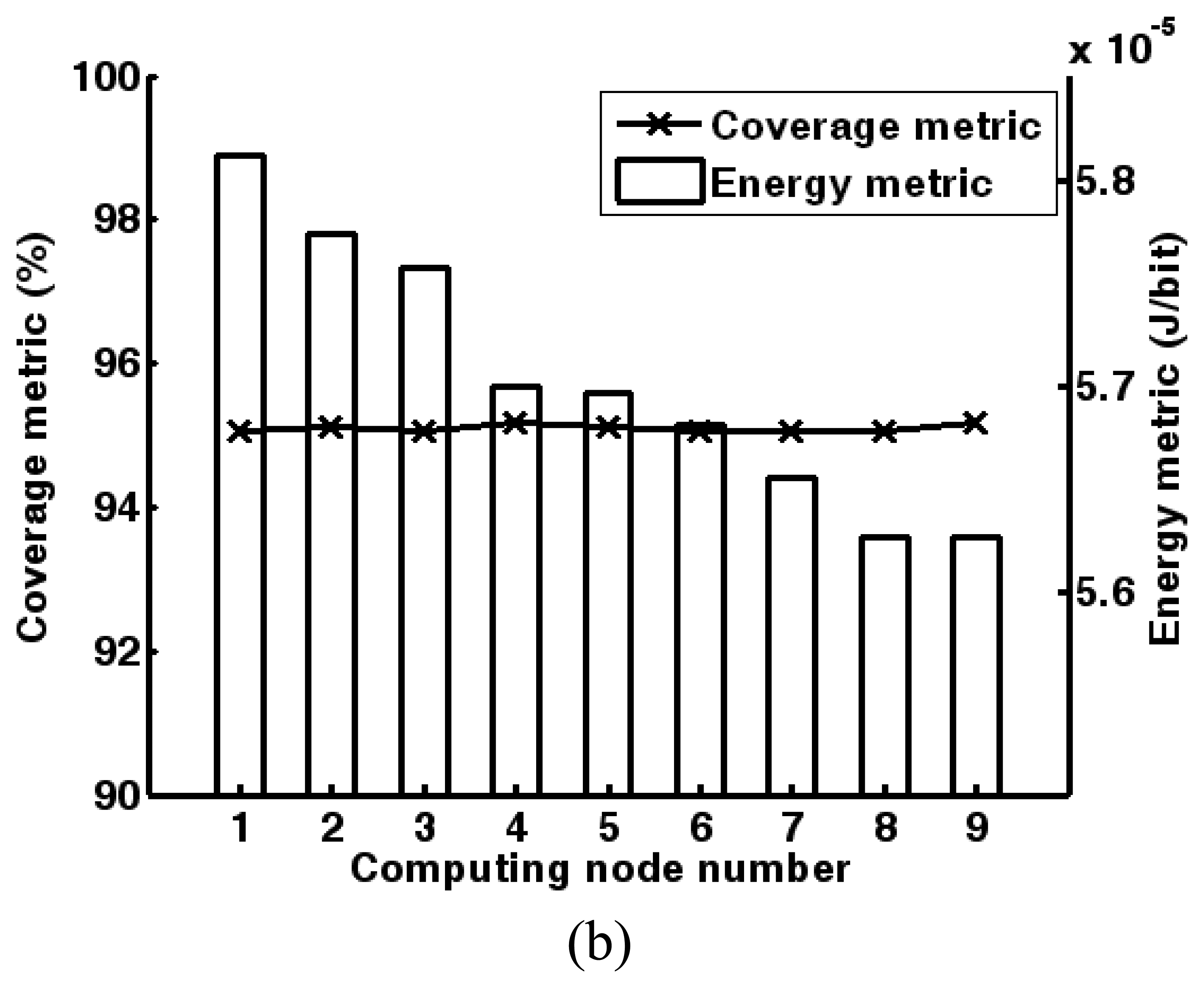
Then, we implement DPSOSA to optimize the deployment of WSN with a different computing node number
SA_NUM, which varies from 1 to 9. Specially, the algorithm is accomplished by the sink node when
SA_NUM is set as 1. Since each wireless sensor node has little information to exchange with the sink node and the computing node number is limited during DPSOSA, its communication cost can be ignored. As shown in
Figure 4, the optimization results of DPSOSA are obtained under the two kinds of coverage requirement. We can find that all the optimized coverage metrics exceed 95%, while the energy metric trends to be lower as the computing node number becomes larger. Hence, the performance of DPSOSA benefits from the computation capacity of multiple wireless sensor nodes.
To obtain ideal optimization results, the computing node number is fixed as 9 in the following discussion. Then,
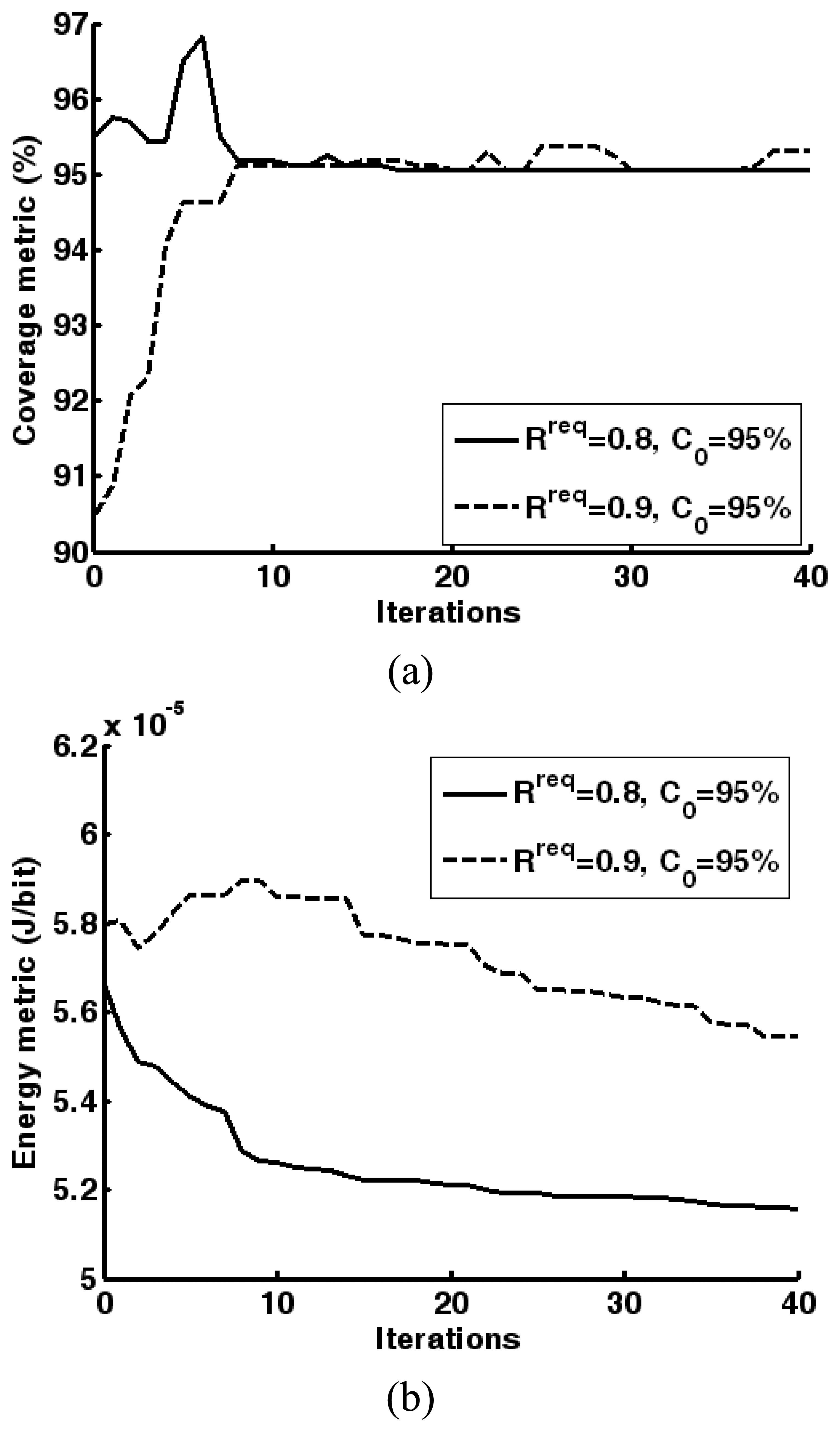
Figure 5 shows the convergence curves of the metrics under the two kinds of coverage requirement. Rather than the coverage requirement that
Rreq = 0.8 and
C0 = 95%, it is more difficult to achieve the coverage requirement that
Rreq = 0.9 and
C0 = 95%. Therefore, the former coverage requirement is satisfied at the beginning, while the latter one is satisfied after 8 iterations in the optimization procedure, which is shown in
Figure 5(a). In
Figure 5(b), the algorithm can make more effort to achieve improved energy metric with the former coverage accordingly. Meanwhile, the former coverage requirement provides more adjustability for mobile node deployment to achieve lower energy metric.
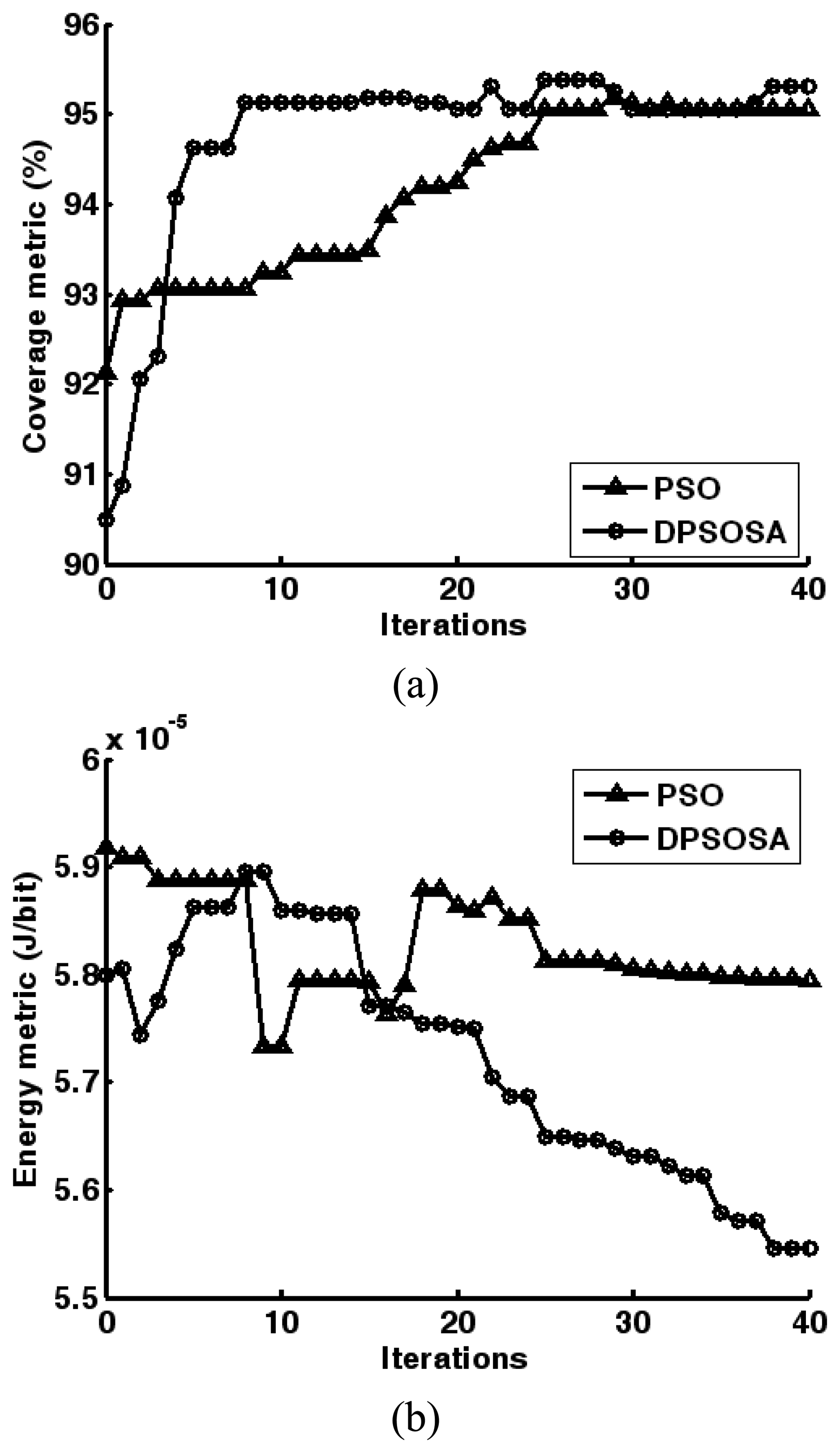
Furthermore, we will compare the performance of DPSOSA and general PSO algorithms. Here, only the coverage requirement that
Rreq = 0.9 and
C0 = 95% is considered. The same scenario and fitness function is employed in PSO. In
Figure 6, the convergence curves of coverage and energy metrics are presented during DPSOSA and PSO. From
Figure 6(a), we can find that PSO spends much more iterations than DPSOSA to satisfy the coverage requirement though it has a better initial coverage of mobile nodes. And the energy metric is significantly improved by DPSOSA compared to the optimization result of PSO as shown in
Figure 6(b).
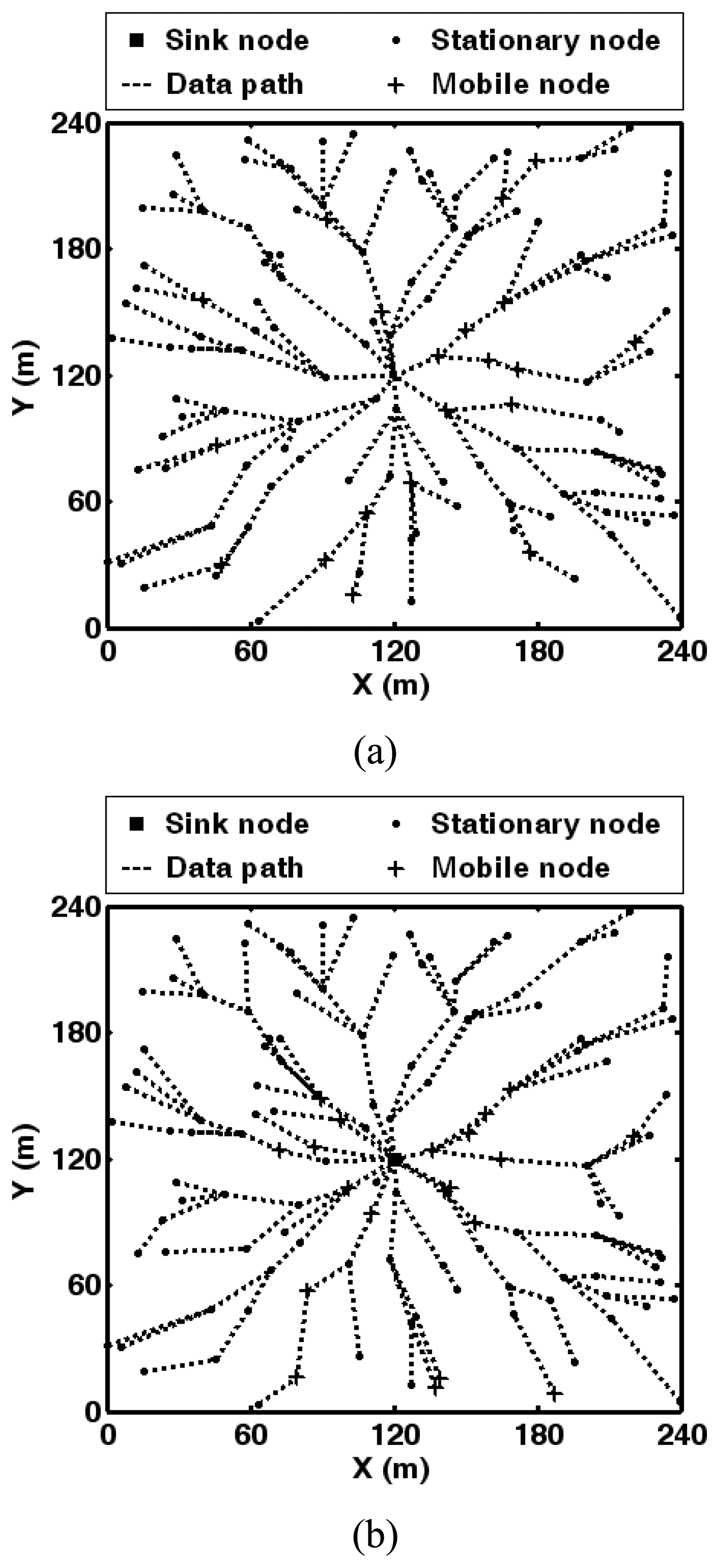
According to the optimization results of PSO and DPSOSA, we can obtain optimized deployment and communication paths of WSN as shown in
Figure 7. The coverage ratio of the WSN in
Figure 7(a) and (b) is 95.13% and 95.31%, respectively. It can be seen that the data paths obtained by DPSOSA tend to provide more potential for multi-hop communication instead of using longer distance data transmission, although both algorithms attempt to achieve energy efficiency. As a result, the energy metrics obtained by PSO and DPSOSA are 5.83 × 10
−5J/
bit and 5.57 × 10
−5J/
bit, respectively.
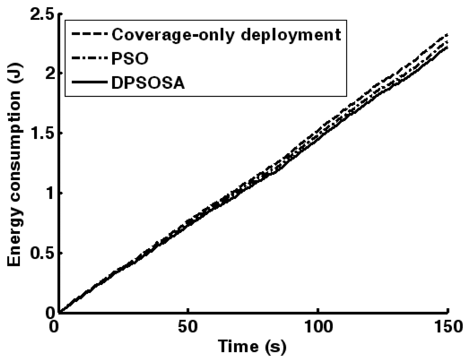
Finally, scenarios of WSN are set up according to
Figure 7(a) and (b) for target tracking simulations. Besides, we discuss a coverage-only deployment, which is optimized by DPSOSA taking only coverage metric into account. In each sensing period, the closest wireless sensor node to the mobile target is chosen via negotiation. It then acquires information and sends a 2KB data packet to the sink node along the optimized path. The total energy consumption over time is extracted from the simulations, as shown in
Figure 8. We find that the WSN optimized by DPSOSA has a lower energy consumption than the one optimized by PSO. Moreover, target tracking is a long term task, so more energy could be saved during the lifetime of WSNs. Compared to the coverage-only deployment, DPSOSA achieves an energy conservation of 4.68%.
From the experiments, the efficiency of multiple computing nodes is verified and it is shown that DPSOSA can applied under different coverage requirements. Then, the improved energy efficiency of DPSOSA is demonstrated by algorithm simulations and target tracking application compared with general PSO.
6. Conclusions
Focusing on the energy-efficient coverage problem of WSNs, this paper has proposed distributed particle swarm optimization and simulated annealing to optimize the network deployment. In a network composed of stationary and mobile wireless sensor nodes, the proper placement of mobile nodes is discussed, considering sensing coverage and energy consumption. Then, the coverage metric is defined utilizing a grid exclusion algorithm, while the energy metric is calculated by Dijkstra's algorithm, which provides the optimal communication paths for data reporting. Particle swarm optimization and simulated annealing are combined to find the global optimal solution, where the fitness function is designed to minimize the energy metric guaranteeing specified coverage ratio. Besides, computation capability of multiple wireless sensor nodes is adopted to enhance the optimization capacity. Experimental results represent that significant energy conservation can be achieved by the proposed optimization algorithm compared to general PSO, and energy efficiency of WSN is boosted up in target tracking application. This paper presents an evaluation method for energy-efficiency of coverage problem in WSNs. The application-oriented property is realized by target tracking. Still, further investigation should be made on adaptive routing schemes and scalable network topologic.


