Simulated Effects of Soil Temperature and Salinity on Capacitance Sensor Measurements

Abstract

Dielectric measurement techniques are used widely for estimation of water content in environmental media. However, factors such as temperature and salinity affecting the readings require further quantitative investigation and explanation. Theoretical sensitivities of capacitance sensors to liquid salinity and temperature of porous media were derived and computed using a revised electrical circuit analogue model in conjunction with a dielectric mixing model and a finite element model of Maxwell's equation to compute electrical field distributions. The mixing model estimates the bulk effective complex permittivities of solid-water-air media. The real part of the permittivity values were used in electric field simulations, from which different components of capacitance were calculated via numerical integration for input to the electrical circuit analogue. Circuit resistances representing the dielectric losses were calculated from the complex permittivity of the bulk soil and from the modeled fields. Resonant frequencies from the circuit analogue were used to update frequency-dependent variables in an iterative manner. Simulated resonant frequencies of the capacitance sensor display sensitivities to both temperature and salinity. The gradients in normalized frequency with temperature ranged from negative to positive values as salinity increased from 0 to 10 g L^-1. The model development and analyses improved our understanding of processes affecting the temperature and salinity sensitivities of capacitance sensors in general. This study provides a foundation for further work on inference of soil water content under field conditions.

1. Introduction

Capacitance-based electronic instruments are gaining common application in the field for estimation of soil water content from bulk dielectric properties. Such instruments are generally sensitive to several factors, including soil temperature and electrical conductivity, affecting the effective complex permittivity of environmental media surrounding the probe. Temperature-dependence of the measured bulk permittivity and apparent water content has been observed in the laboratory [1-8]. Thereby, possible effects caused by temperature sensitivity of the instrumental electronics have been recognized for different transmission line-type electromagnetic methods [4, 9, 10]. Experiments under field conditions have also been conducted to infer temperature effects on capacitance measurements [11].

Baumhardt et al. [3] conducted greenhouse experiments in soils under diurnal soil temperature fluctuations. Bulk soil electrical conductivities were on the order of 100 mS m^-1. They demonstrated that the capacitance probes were sensitive to both temperature and electrical conductivity, where a fluctuation of approximately 15°C caused a fluctuation in the apparent soil water content of 0.04 m³ m^-3 based on the default calibration of the Sentek EnviroSCAN^™ instrument relating sensor readings to soil water content. Subsequently, Evett et al. [12] reported a temperature dependence dθ / dT of 0.0005 to 0.0017 m³ m^-3 K^-1 using factory and soil-specific calibrations.

Despite advances in the theory [4, 13-15], the mechanisms for dielectric loss in porous multi-phase media (soils) over a broad range of frequencies are complicated [16], such that a simple correction for temperature may not be possible [5]. Kelleners et al. [14] used electrical circuit theory as an analogue to describe the capacitance sensor in terms of a resistor-capacitor-inductor (RCL) circuit, where electrical conductivity of test liquids was shown to decrease the resonant frequency. Likewise, Robinson et al. [15] identified a decrease in the resonant frequency with increasing electrical conductivity under isothermal conditions using a different probe configuration (a surface capacitance insertion probe).

There remains a practical need for methods to compensate for temperature effects in soils of various bulk electrical conductivities, especially in shallow applications where temperature and water content fluctuations can be significant. Physics-based theory and methods as presented in this work are needed to predict a range of environmental conditions where temperature and electrical conductivity can affect instrumental measurements used to estimate soil water content.

1.1 Previous Sensor Applications and Testing

The present theoretical developments are meant to be as generic as possible, while the capacitance sensor geometry is specific to a commercial device: Sentek capacitance sensors used on EnviroSMART^™ and EnviroSCAN^™ probes. Both probes are inserted vertically inside a plastic access tube such that the outside diameter of the access tube contacts the surrounding media (soil). Figure 1 shows a cross-section of the sensor geometry. More detailed descriptions and images have been reported in previous studies performed in the laboratory [17,18] and field [19].

1.2 Conversion of Frequency Measurements to Permittivities

The normalized sensor reading N derived from the resonant frequency f_r is a dimensionless number (also known as “scaled frequency”):

$$N\equiv \frac{f_{\text{r},\text{a}}-f_{\text{r}}}{f_{\text{r},\text{a}}-f_{\text{r},\text{w}}}$$

(1)

where f_r,a and f_r,w are the resonant frequencies measured in air and pure water at the reference temperature T_ref = 20°C with corresponding environmental permittivities ε_a = 1 and ε_w′ = 80.2 (real part valid for 100 - 250 MHz). According to the above definition, the normalized reading is N = 0 for an air reading and N = 1 for a measurement in pure water at temperature T = T_ref.

The relation ε̂ (N) between the permittivity ε̂ of environmental media surrounding the access tube and N was determined experimentally in a laboratory characterization of the sensor presented in Schwank et al. [18]:

$$\widehat{\epsilon }(N)=\left({\epsilon }_{\text{a}}+\left({{\epsilon }^{\prime }}_{\text{w}}{e}^{-k}-1-a_2\right)N+a_2{N}^2\right)\cdot e^{kN}$$

(2)

The experiments leading to this empirical relation were performed in almost lossless mixtures of water and dioxane (1,4-diethylene dioxide: C₄H₈O₂) with real permittivities in the range of 2.4 ≤ ε̂ ≈ ε_m′ ≤ 78.4; and the fitting parameters were determined as a₂ = 1.12819 and k = 6.64846. The parameters were optimized to fit permittivities in the range applicable to bulk soil-water-air mixtures (4 < ε_m′ < 40), such that (2) is not intended for applications in pure water. Combining (1) with (2) allows for estimation of ε_m′ ≈ ε̂ of a non-conducting medium from f_r measured with the capacitance sensor. However, in a conducting medium the measurement based ε̂ (N) is expected to deviate significantly from the value ε_m′ which is inherently independent of the medium conductivity.

2. Methods

The resonant frequency f_r(ε_m) of a capacitance sensor is affected by the complex permittivity ε_m = ε_m′ + i ε_m″ of the medium (soil) surrounding the probe. The positive imaginary part used in this notation is the consequence of the negative time factor exp(-i ω t) generally used by physicists for representing wave functions, where $\text{i}\equiv \sqrt{-1}$. The bulk soil electrical DC-conductivity σ_m, volumetric water content θ, and temperature T of the soil medium affect both the real and the imaginary parts ε_m′ and ε_m″. Because the salinity S of the liquid phase affects σ_m, the resonant frequency f_r response of the capacitance probe is sensitive to θ, S, and T specifying the bulk soil status.

The approach to predict f_r(θ, S, T) is based on linking three types of models. First, the electrical circuit analogue shown in figure 1 is used to represent the capacitance sensor which is based on a resonance phenomenon. Second, an effective medium approach is used to estimate the frequency-dependent complex effective permittivity ε_m(f) of the bulk soil surrounding the probe for given θ, S, and T. Third, Maxwell's equations are solved numerically to derive the electrical field E caused by the sensor configuration for the environmental permittivity ε_m(f). The values of the circuit analogue elements (figure 1) are then computed from E. Fourth, the electrical circuit analogue model is solved for f_r. If the bulk soil is considered as a dispersive medium with frequency-dependent ε_m(f), the sensor resonance f_r has to be determined iteratively as illustrated in figure 2.

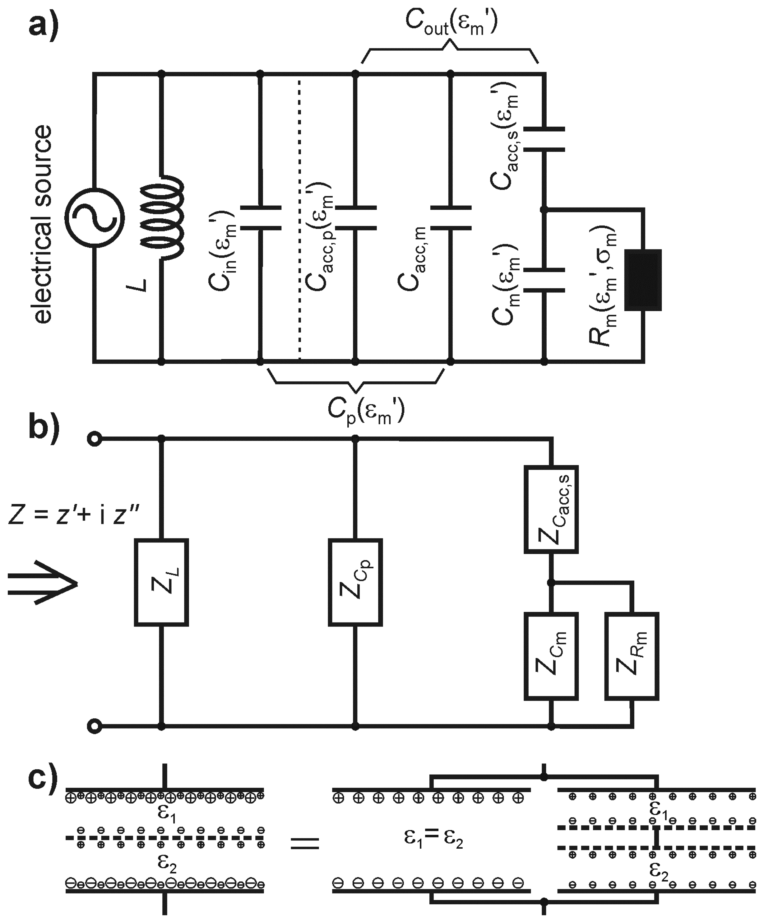
2.1 Electrical Circuit Analogue

The frequency response of the capacitance sensor is modeled using a detailed circuit analogue with more components of capacitance than the one used by Kelleners et al. [14] and a resistor, which was neglected by Schwank et al. [18] in the absence of significant dielectric losses. The arrangement of the circuit diagram components considered here and assumed to represent the spectral characteristics of the sensor are shown in figure 1a.

The electrical source and the inductance L are part of the sensor electronic board which is mounted inside the sensor electrode rings. The value of the inductance L is calculated from the measured coil length l = 4 mm, mean diameter d = 3.5 mm, and the number of turns n = 6.5 such that L = F·n²d = 91.95 nH with the factor F = 0.62181 given in Terman [20, pp. 53-54]. The total capacitance C_tot is composed of inner and outer capacitances with respect to the ring electrodes acting in parallel. These partial capacitances are associated with different volumes in the vicinity of the sensor electrodes.

Figure 3a provides a close-up view of the ring-capacitor sensor with symbolized electric field E spreading through the access tube into the media (soil). The dashed lines indicate the axes of symmetry in the vertical, z, and radial horizontal, r, directions. In Fig. 3b the sensor geometry used for the simulations is shown in cross-section. The inner capacitance C_in is caused by the sensor volume with r ≤ r_acc,in = 1 inch (25.4 mm) inside the access tube. This volume includes the axisymmetric electrode holder and also the electronic board and wiring, which are not axisymmetric. The capacitance caused by the access tube volume r_acc,in < r < r_acc,out is separated into a parallel part C_acc,p and a serial part C_acc,s with respect to the electrical source. The volume outside the access tube (r > r_acc,out) is represented by the capacitance C_m with an electrical resistance R_m in parallel for taking into account the conductivity losses of the medium (soil).

The series capacitors C_acc,s and C_m are interpreted as distinct capacitances by virtue of a double layer of electrical charges accumulated at the dielectric discontinuity at the outer access tube boundary r = r_acc,out associated with the unequal polarization within and beyond the access tube. The polarization P (and the electrical field E) at r = r_acc,out is continuous if the permittivities ε_acc and ε_m of the access tube and the medium are equal, so by definition C_acc,s and C_m do not exist in this case (i.e., in the limit ε_m → ε_acc: C_acc,s = C_m = 0 pF). However, the capacitance between the ring-electrodes caused by the volume r > r_acc,in comprising the access tube and the medium, is certainly not zero for ε_acc = ε_m. For this purpose, the capacitor C_acc,m is introduced to account for the parallel capacitance at ε_acc=ε_m caused by the volume confined by r > r_acc,in.

A symbolic justification of the necessity for introducing C_acc,m is sketched in figure 1c where the role of two partial capacitances given by two dielectric regions ε₁, ε₂ within a composite plate capacitor is illustrated. The large circles with the plus and minus signs symbolize electrical charges on the conducting electrodes of the capacitor associated with ε₁ = ε₂, whereas the corresponding small circles are the charges of the double-layer accumulated at the non-conducting dielectric discontinuity. As it is depicted, the capacitance of the composite capacitor is represented by a capacitor with uniform dielectric ε₁ = ε₂ (corresponding to C_acc,m) in parallel with the series of two capacitors with permittivities ε₁ and ε₂ (corresponding to C_acc,s and C_m).

The resonant frequency f_r of the circuit analogue is derived by applying Complex AC-Circuit Theory [20] to the circuit analogue shown in figure 1b. Complex AC-Circuit Theory states that the impedance Z = z′ + i z″ of a circuit composed of passive elements R [Ω] (resistor), L [H] (inductance), and C [F] (capacitance) can be described using Ohm's-law if corresponding frequency-dependent complex impedances Z_R, Z_L and Z_C are used:

$$Z_{\text{R}}=R,Z_{\text{L}}=\text{i}2\pi f\cdot L,\text{and}{Z}_{\text{C}}=\frac{-\text{i}}{2\pi f\cdot C}$$

(3)

Consequently, the impedance Z(f) of the circuit depicted in figure 1b can be expressed by the impedances Z_Rm, Z_L, Z_Cacc,s, Z_Cm, and Z_Cp where C_p = C_in + C_acc,p + C_acc,m is in parallel to the electrical source:

$$Z(f)={\left[Z_{\text{L}}^{-1}+Z_{{\text{C}}_{\text{P}}}^{-1}+{\left({\left(Z_{{\text{C}}_{\text{m}}}^{-1}+Z_{{\text{R}}_{\text{m}}}^{-1}\right)}^{-1}+Z_{\text{acc},\text{s}}\right)}^{-1}\right]}^{-1}$$

(4)

The circuit is operated at its resonant frequency f = f_r if the energy uptake is maximal, i.e., if the input impedance Z(f = f_r) takes a real value. The physically meaningful solution of the corresponding equation z″(f = f_r) = 0 is:

$$f_{\text{r}}=\frac{1}{2\pi \sqrt{2}}\sqrt{\frac{-\left(C_{\text{acc},\text{s}}+C_{\text{p}}\right)L+{\left(C_{\text{acc},\text{s}}+C_{\text{m}}\right)}^2{R}_{\text{m}}^2+\sqrt{D}}{\left(C_{\text{acc},\text{s}}+C_{\text{m}}\right)\left(C_{\text{m}}{C}_{\text{p}}+C_{\text{acc},\text{s}}\left(C_{\text{m}}+C_{\text{p}}\right)\right)L{R}_{\text{m}}^2}}$$

with

$$D={\left(C_{\text{acc},\text{s}}+C_{\text{p}}\right)}^2{L}^2+{\left(C_{\text{acc},\text{s}}+C_{\text{m}}\right)}^4{R}_{\text{m}}^4-2\left(C_{\text{acc},\text{s}}+C_{\text{m}}\right)\left(C_{\text{acc},\text{s}}^2-C_{\text{m}}{C}_{\text{p}}-C_{\text{acc},\text{s}}\left(C_{\text{m}}+C_{\text{p}}\right)\right)L{R}_{\text{m}}^2$$

(5)

The above expression f_r(L, C_p, C_acc,s, C_m, R_m) is used to calculate the resonance of the circuit analogue (figure 1). For the limits of a lossless (R_m → ∞) and a highly conducting (R_m → 0) medium the expression (5) reduces to the formula valid for a simple LC-oscillator.

$$f_{\text{r}}=\frac{1}{2\pi \sqrt{LC}}$$

(6)

Thereby, the operative capacitance for the lossless case (R_m → ∞) is C = C_p + (C_acc,s · Cm) / (C_acc,s + C_m) representing the total input-capacity of the circuit diagram without the presence of the resistor R_m. In the limit R_m → 0 one finds the larger value C = C_p + C_acc,s representing the corresponding operative capacitance for hot-wired C_m. These considerations already show that f_r is expected to increase with R_m between the two limits for R_m → 0 and R_m → ∞.

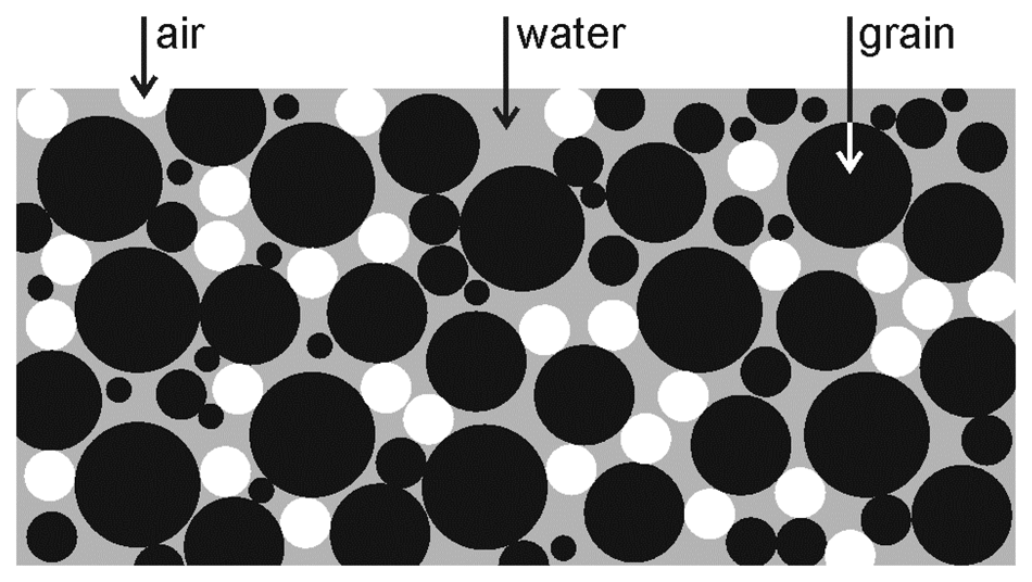
2.2 Electrical Properties of Porous Media

The effective permittivity ε_m = ε_m′ + i ε_m″ and the electrical DC-conductivity σ_m of the media surrounding the sensor are described on the basis of a physical dielectric mixing approach. Thereby, the effective permittivity ε_m is defined using the relation <D> = ε_m <E> between the flux density D and the electrical field E, where < > denotes a linear volume average over all dielectric phases. From these basic considerations, a generalized form of the Maxwell-Garnett formula [21, 22] can be derived to compute ε_m of a multiphase mixture comprising K different types of spherical inclusions:

$${\epsilon }_{\text{m}}={\epsilon }_{\text{e}}+3{\epsilon }_{\text{e}}\frac{\sum _{j=1}^k{v}_j\frac{{\epsilon }_j-{\epsilon }_{\text{e}}}{{\epsilon }_j+2{\epsilon }_{\text{e}}}}{1-\sum _{j=1}^k{v}_j\frac{{\epsilon }_j-{\epsilon }_{\text{e}}}{{\epsilon }_j+2{\epsilon }_{\text{e}}}}$$

(7)

Thereby, only the volume fraction v_j of the guest phases with permittivities ε_j and the permittivity ε_e of the host appear in the mixing formula. In fact, the assumption that the spheres in the mixture be of the same size can be relaxed as long as all spheres are small compared with the wavelength of the operating electrical field. Because this effective medium approach is derived directly from basic electromagnetism, it can be applied for complex permittivity values ε_j and ε_e without any restrictions.

We applied the mixing rule (7) to the simplified model structure depicted in figure 4 for modeling the permittivity ε_m = ε_m′ + i ε_m″ of the porous medium representing the bulk soil with porosity η and volumetric water content θ. This dielectric mixture accounts for spherical grains and air bubbles with permittivities ε_g and ε_a = 1 embedded in the water phase with permittivity ε_w. Accordingly, Equation (7) has to be evaluated for K = 2 with the corresponding volume fractions 1 - η and η - θ of the grain- and of the air-phase respectively:

$${\epsilon }_{\text{m}}={\epsilon }_{\text{w}}+3{\epsilon }_{\text{w}}\frac{(1-\eta )\frac{{\epsilon }_{\text{g}}-{\epsilon }_{\text{w}}}{{\epsilon }_{\text{g}}+2{\epsilon }_{\text{w}}}+(\eta -\theta )\frac{{\epsilon }_{\text{a}}-{\epsilon }_{\text{w}}}{{\epsilon }_{\text{a}}+2{\epsilon }_{\text{w}}}}{1-\left[(1-\eta )\frac{{\epsilon }_{\text{g}}-{\epsilon }_{\text{w}}}{{\epsilon }_{\text{g}}+2{\epsilon }_{\text{w}}}+(\eta -\theta )\frac{{\epsilon }_{\text{a}}-{\epsilon }_{\text{w}}}{{\epsilon }_{\text{a}}+2{\epsilon }_{\text{w}}}\right]}$$

(8)

The above mixing approach is best for sandy soils at relatively high water contents, where the water phase is the host of nearly spherical air bubbles. Complex air-water geometries at low water contents might be not described properly by (8). Furthermore, for very fine textured soils (clays) with high specific surface areas (up to ≈ 200 m²g^-1) the above mixing model is improper due to relaxation phenomena like Maxwell-Wagner or due to the increasing fractional amount of bound water becoming a further dielectric phase to be considered [23].

The constant value ε_g = 5.5 + i 0.2 is reasonable for the permittivity of silicon dioxide (SiO₂, quartz) [24] which is most abundant in natural sands. The complex permittivity of water ε_w = ε_w′ + i ε_w″ is computed from a fit of measurements performed at frequency f, water temperature T and salinity S. The multi-parameter fit for ε_w(f, T, S) described by Meissner and Wentz [25] consists of a double Debye relaxation law for expressing the explicit frequency dependence of ε_w. The T and S dependencies are formulated implicitly by making the involved Debye parameters (static-, intermediate-, and high-frequency dielectric permittivity and two relaxation frequencies) dependent on T and S. The electrical DC-conductivity σ_w(T, S) of the saline water, used in the conductivity-term of the fitting approach, is calculated using a fit to measurements, where salinity is expressed in parts per thousand (ppt) by weight, which at low concentrations is approximately equal to grams (g) of salt per liter (L) of water. We followed the empirical derivations of Meissner and Wentz [25], who assumed the salinity of sea water was dominated by monovalent cations, which affects the conversion from mass concentration in ppt to electrical conductivity of the solutions.

The validity of the semi-empirical model for ε_w(f, T, S) holds for the following ranges: f ≤ 90 GHz, -2°C ≤ T ≤ +29°C, S ≤ 40 ppt. However, for pure water (S = 0) the fit is based on measurements taken within the broader temperature range -21°C ≤ T ≤ +40°C. As a consequence, the upper temperature limit of the applicability of the fit ε_w(f, T, S) is expected to be broader for low salinities S ≤ 10 ppt used in our evaluations.

The DC-conductivity σ_m of a medium can be deduced from ε_m by expressing the spectral properties of ε_m as the sum of a conductivity term comprising σ_m, the constant ε_{m ∞} representing the high-frequency limit, and a Debye relaxation term. The Debye term considers the rotational relaxation frequency f_rel ≫ 1 GHz (figure 5) and low- and high-frequency limits, ε_{m DC} and ε_{m ∞}, respectively. The conductivity term describes the steadily increasing (hyperbolic) losses for frequencies f < 1 GHz contributing exclusively to ε_m″. The frequency spectrum of ε_m(f) is thus (ε₀ = 8.85 10^-12 F m^-1):

$${\epsilon }_{\text{m}}(\text{f})=\frac{{\epsilon }_{\text{m DC}}-{\epsilon }_{\text{m}\infty }}{1-\text{i}f/f_{\text{rel}}}+{\epsilon }_{\text{m}\infty }+\text{i}\frac{{\sigma }_{\text{m}}}{{\epsilon }_{0}2\pi f}$$

(9)

Here, relaxation losses can be neglected, because the frequencies of the electric field (100 – 160 MHz) excited by the considered capacitance sensor are much smaller than 1 GHz (f ≪ f_rel). Thus, the DC-conductivity σ_m(ε_m″, f) is directly proportional to the imaginary part ε_m″(f) of the medium permittivity measured at the frequency f:

$${\sigma }_{\text{m}}\left({\epsilon }_{\text{m}}^{″},f\right)={\epsilon }_{0}2\pi f{\epsilon }_{\text{m}}^{″}$$

(10)

As a matter of clarification, the fact that the above expression involves f does not mean that the DC-conductivity σ_m is frequency dependent, because ε_m″ is inversely proportional to f.

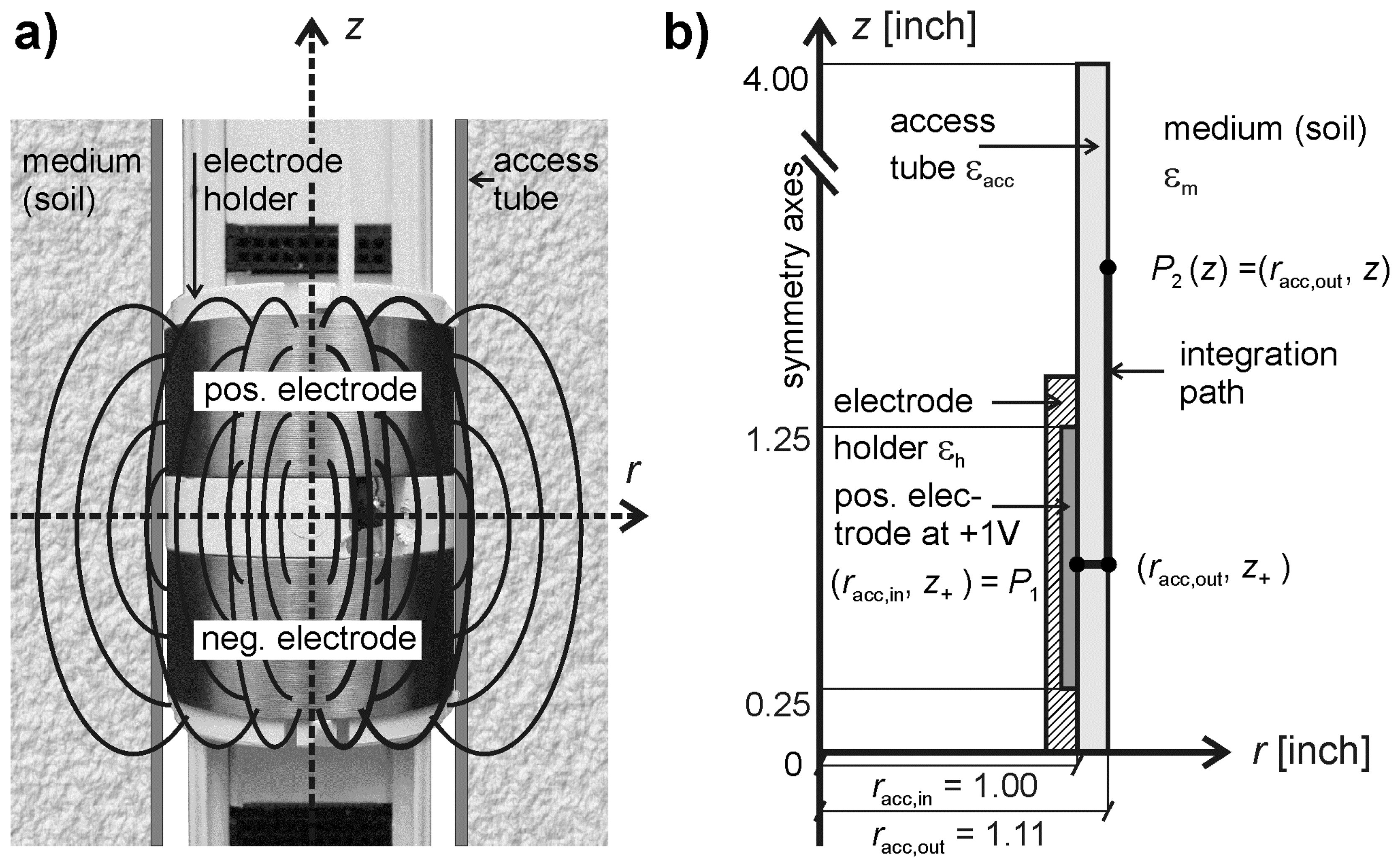
2.3 Electric Field Simulations

Schwank et al. [18] introduced the use of a numerical simulator to compute the electric field distributions within and around an axisymmetric capacitance sensor. Electrical fields E were simulated using the free version of the commercial finite element software Maxwell®2D, which can be downloaded from http://www.ansoft.com/maxwellsv/.

The model geometry implemented in the numerical simulation for computing E in the vicinity of the two ring electrodes is depicted in figure 3b. The sketch utilizes the rotationalsymmetry around the z-axis of the sensor and the mirror symmetry with respect to the plane perpendicular to z in the middle of the two ring electrodes. With respect to these symmetry properties, the fields were calculated in cylindrical coordinates yielding E(r, z) = (E_r, E_z) in radial and tangential components. The simulations were performed within the volume confined by 0 ≤ r ≤ r_max and -z_max ≤ z ≤ z_max with r_max = 8 inches (203 mm) and z_max = 4 inches (102 mm) for the potential difference U_± = 1 V applied between the ring electrodes of the sensor. Furthermore, the permittivities of the access tube and of the electrode holder were set to ε_acc = ε_h = 3.35 in accordance with measured values for f ≤ 1 GHz [18]. Quasi-steady field solutions E(r, z) were computed for a set of real media permittivities ε_m′ in the range 3.35 = ε_acc ≤ ε_m′ ≤ 80. It has been proven numerically that an imaginary part ε_m″ ≠ 0 of ε_m does not alter the values of E(r, z) and the quasi-steady field approximation is justified as the relevant wavelengths of the electrical field are clearly larger than the dimensions of the volume considered in the simulations.

The recursion proceeded until reaching the targeted change of 0.01 % of the total field energies of subsequent iterations. Meeting this stopping criterion typically required 10 grid points in the adaptive finite-element mesh. The modeled fields E(r, z) were then used to calculate the circuit diagram elements C_in(ε_m′), C_acc,p(ε_m′), C_acc,m, C_acc,s(ε_m′), C_m(ε_m) and R_m(ε_m′, ε_m″) for the permittivity range 3.35 = ε_acc ≤ ε_m′ ≤ 80.

2.4 Components of the Circuit Diagram

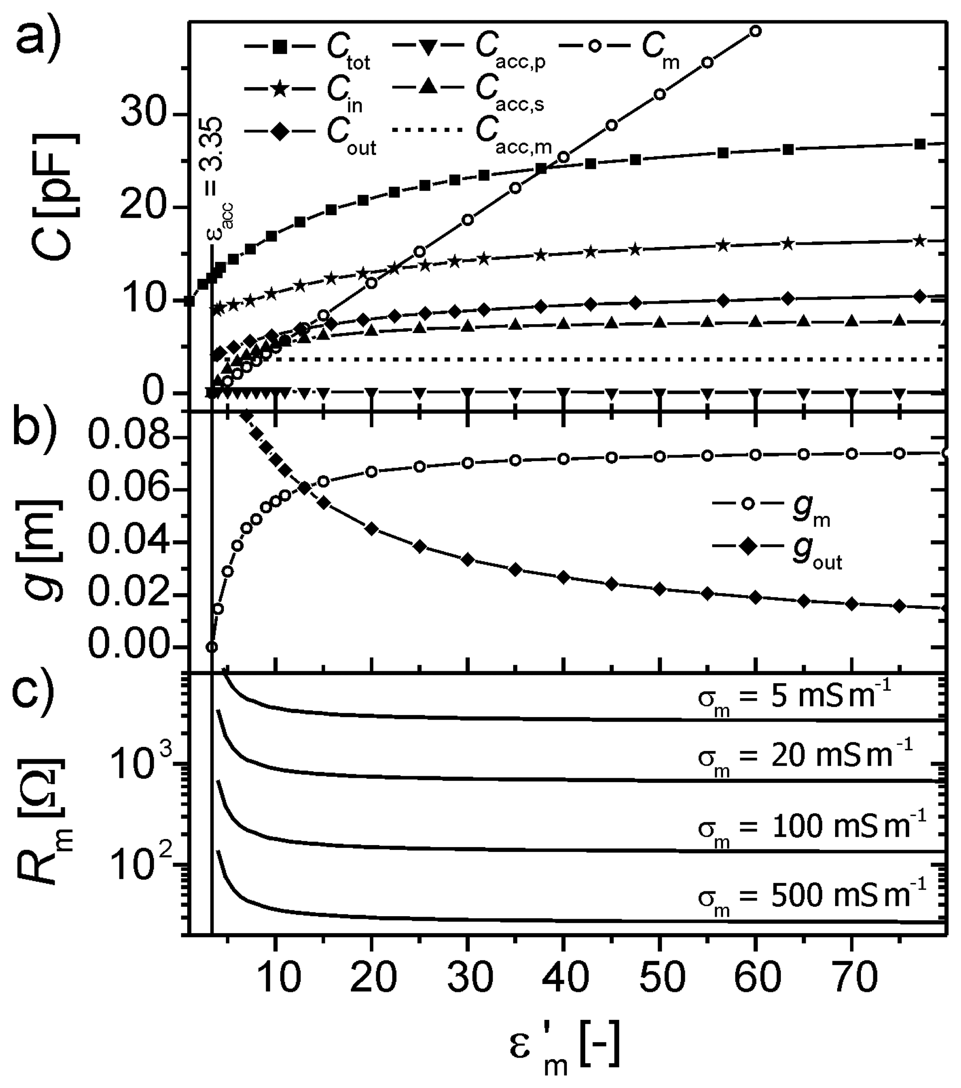
2.4.1 Capacitances

The total capacitance C_tot was first decomposed into two basic parallel capacitance components associated with the volumes V_in and V_out confined by r ≤ r_acc,in and r > r_acc,in (compare figure 1 and 3):

$$C_{\text{tot}}=C_{\text{in}}+C_{\text{out}}$$

(11)

Based on the circuit analogue, the capacitance C_out caused by the axisymmetric volume V_out is:

$$C_{\text{out}}=C_{\text{acc},\text{p}}+C_{\text{acc},\text{m}}+\frac{C_{\text{acc},\text{s}}{C}_{\text{m}}}{C_{\text{acc},\text{s}}+C_{\text{m}}}$$

(12)

As will be explained below the capacitances C_acc,m, C_acc,s, C_m, C_acc,p, and C_out were computed from the field E(r, z) simulated for ε_m′. These capacitance values ultimately were used for computing f_r(L, C_p, C_acc,s, C_m, R_m) from (5). Also, the capacitance C_p used in (5) is the parallel connection of three capacitors (figure 1a):

$$C_{\text{p}}=C_{\text{in}}+C_{\text{acc},\text{p}}+C_{\text{acc},\text{m}}$$

(13)

Because the field caused by the asymmetric wiring and the electronic board cannot be simulated with the two-dimensional finite element software, C_in was derived from the difference between the measured total capacitance C_tot and the simulated capacitance C_out. Simulated and measured values of C_tot(ε_m′) deviate significantly from each other as shown in Schwank et al. [18]. Internal asymmetrical material (electronic board, wiring) plus on-board capacitance of the electronics were identified as the main reason for the inaccuracy of the simulations. Thus, C_tot(ε_m′) used in (11) is derived from the experimental data (Schwank et al. [18], figure 8) measured in water-dioxane mixtures (2.4 ≤ ε_m′ ≤ 78.4) and corrected for the effect of the Fluorinated Ethylene-Propylene (FEP) coating (figure 11a in Schwank et al. [18]).

The capacitance C_out(ε_m′) due to the volume outside the access tube is calculated from the field energy ϕ_out within the volume V_out given by r > r_acc,in. Thereby, ϕ_out equals the volume integral of the scalar product of the E-field and the flux-density D:

$${\varphi }_{\text{out}}=\frac{1}{2}\underset{V_{\text{out}}}{\int }\mathbf{\text{E}}\cdot \mathbf{\text{D}}dV$$

(14)

Furthermore, ϕ_out is related to the electrode potential difference U_± and the capacitance C_out:

$${\varphi }_{\text{out}}=\frac{C_{\text{out}}{U}_{\pm }^2}{2}$$

(15)

Combining (14) with (15) allows for calculating C_out(ε_m′) from the field E(r, z) = (E_r, E_z) simulated for ε_m′. The special case when ε_m′ = ε_acc = 3.35 yields the value C_acc,m = C_out(ε_m′ = ε_acc) = 3.63 pF.

C_m(ε_m′) and C_acc,s(ε_m′) can not be calculated using (14) and (15), because these capacitances are not defined between two conducting electrodes but between an electrode and the dielectric discontinuity at the outer boundary of the access tube. However, C_m and C_acc,s can still be computed from E(r, z) = (E_r, E_z) if understood to be the parallel connection of infinitesimal capacitances dC_m(z) and dC_acc,s(z) given by appropriate pairs of surface elements at the outer access tube boundary with radius r_acc,out. Thus, for ring surfaces with radius r_acc,out located at ± z relative to the mirror-symmetry of the sensor, we get:

$${\text{C}}_{\text{m}}=\underset{Z=0}{\overset{\infty }{\int }}d{C}_{\text{m}}(z)\text{and}{C}_{\text{acc},\text{s}}=\underset{Z=0}{\overset{\infty }{\int }}d{C}_{\text{acc},\text{s}}(z)$$

(16)

The infinitesimal capacitances dC_m(z) and dC_acc,s(z) are given by the infinitesimal charge dq(z) accumulated at the ring-shaped surface at z, the voltage u_m(z) between the two mirrored surface elements at ± z, and the voltage u_acc,s(z) between the positive ring-electrode and the outer access tube surface at height z:

$$d{C}_{\text{m}}(z)=\frac{dq(z)}{u_{\text{m}}(z)}\text{and}d{C}_{\text{acc},\text{s}}(z)=\frac{1}{2}\frac{dq(z)}{u_{\text{acc},\text{s}}(z)}$$

(17)

The factor 1/2 is due to the fact that dC_acc,s is the series of two identical capacitances joined at the symmetry plane.

According to Kirchhoff s voltage law, u_m(z) and u_acc,s(z) can be expressed by the electrode potential difference U_± and the voltage U_+P2(z) between the positive electrode and the outer access tube surface element at P₂(z) = (r_acc,_out, z) (figure 3b):

$$u_{\text{m}}(z)=U_{\pm }-2U_{+P_2}(z)\text{and}{u}_{\text{acc},\text{s}}(z)=U_{+P_2}(z)$$

(18)

U_+P2(z) was calculated as the line integral of E(r, z) = (E_r, E_z) from a point P₁= (r_acc,in, z₊) at z₊ within the surface of the positive electrode to the point P₂(z) = (r_acc,out, z). As verified numerically, this integration is path independent because ∇ × E = 0 in the charge-free space within the access tube. Integrating along a convenient path (figure 3b) connecting P₁ with P₂(z) yields:

$$U_{+P_2}(z)=\underset{P_1}{\overset{P_2(z)}{\int }}\mathbf{\text{E}}\cdot d\text{s}=\underset{r_{\text{acc}.\text{in}}}{\overset{r_{\text{acc}.\text{out}}}{\int }}{E}_{\text{r}}(r,z_{+})dr+\underset{z_{+}}{\overset{z}{\int }}{E}_{\text{z}}(r_{\text{acc},\text{out}},z^{\prime })d{z}^{\prime }$$

(19)

For calculating the surface charge density at a dielectric discontinuity, it is appropriate to separate the total volume charge density ρ into parts ρ_u and ρ_p produced by unpaired (u) and paired (p) charges accumulated via charges that can move far away from their partners of opposite sign and by charges accumulated via displacements of paired charges [26]. A polarization P of a dielectric medium causes a paired charge volume density ρ_p= -∇ · P, and the corresponding ρ_u of the free charges is given by the flux density D = ε₀E + P via Gauss's law for electricity ρ_u= ∇·D. Combining these basic relations yields:

$${\epsilon }_0\nabla \cdot \mathbf{\text{E}}={\rho }_{\text{u}}+{\rho }_{\text{p}}$$

(20)

Integrating (20) over an infinitesimal volume enclosing a section of a dielectric discontinuity and using the divergence theorem yields the surface charge densities γ_u and γ_p expressed by the normal components of the fields E₁ and E₂ at both sides of the interface (n̂ = unit-vector normal to the interface;:

$$\widehat{\mathbf{n}}{\epsilon }_0({\mathbf{\text{E}}}_1-{\mathbf{\text{E}}}_2)={\gamma }_{\text{u}}+{\gamma }_{\text{p}}$$

(21)

Because D is continuous across a dielectric discontinuity, the density of unpaired charges is γ_u = 0, whereas the polarization charge density γ_p occurs at a dielectric discontinuity. Therefore, γ_p at the interface separating the access tube from the environmental medium with permittivities ε_m = ε_acc can be calculated from E(r, z). Following the relation (21) and considering the symmetry properties of the sensor and of E(r, z) = (E_r, E_z) with respect to the z-axis, γ_p was determined by the difference between E_r(r, z) at the radii r = r_acc,out − δ and r = r_acc,out + δ where δ is an infinitesimal radius increment.

The resulting infinitesimal charge dq(z) = γ_p·dA used in (17) on a ring-shaped element with area dA = 2π·r_acc,outdz at P₂(z) = (r_acc,out, z) (see figure 3b) on the outer boundary of the access tube is therefore:

$$dq(z)={\epsilon }_0\left[E_{\text{r}}\left(r_{\text{acc},\text{out}}-\delta ,z\right)-E_{\text{r}}\left(r_{\text{acc},\text{out}}+\delta ,z\right)\right]\cdot 2\pi r_{\text{acc},\text{out}}dz$$

(22)

Equations (16) - (22) comprise our method for numerical integration of E(r, z) to compute C_m(ε_m′) and C_acc,s(ε_m′) for ε_m′ ≠ ε_acc (see methods above for ε_m′ = ε_acc).

The parallel part C_acc,p(ε_m′) of the access tube capacitance is calculated from the charge Q_acc,z=0 that would occur on a virtual conductor at the symmetry plane z = 0 of the sensor and the corresponding potential difference U_acc,z=0 to the positive ring electrode:

$$C_{\text{acc},\text{p}}=\frac{1}{2}\frac{Q_{\text{acc},\text{z}=0}}{U_{\text{acc},\text{z}=0}}$$

(23)

Because this virtual conductor coincides with the equipotential at U_acc,z=0 = U_± / 2, it does not affect the field E(r, z) = (Er, Ez). The factor 1/2 in (23) accounts for the fact that C_acc,p is the series of two identical capacitors comprised of the positive ring electrode and the virtual electrode at z = 0. The radial component is E_r = 0 at z = 0, so Q_acc,z=0 can be deduced from E_z(r, z = 0) by integrating the virtual charge density ε₀ · E_z(r, z = 0) on the virtual conductor over the radial extension r_acc,in ≤ r ≤ r_acc,out of the access tube:

$$Q_{\text{acc},\text{z}=0}={\epsilon }_{0}2\pi \underset{r_{\text{acc},\text{in}}}{\overset{r_{\text{acc},\text{out}}}{\int }}{E}_z(r,z=0)r\cdot dr$$

(24)

2.4.2 Resistor

Values of the resistance R_m(ε_m′, ε_m″) of a porous medium outside the access tube (soil) with conductivities σ_m(ε_m″) were derived from E(r, z) = (E_r, E_z) computed for ε_m′ in the corresponding volume V_out (r > r_acc,out). For this purpose a relationship between C_m and R_m is deduced below.

In accordance with (3) the absolute values of local infinitesimal ohmic and capacitive impedances dZ_R and dZ_C can be expressed by corresponding local infinitesimal resistor dR and capacitance dC. For the simplest possible electrode arrangement consisting of infinitesimal parallel electrodes with area dA separated by the distance dD one finds:

$$\left|d{Z}_{\text{R}}\right|=\frac{dD}{dA\cdot {\sigma }_{\text{m}}}\text{and}\left|d{Z}_{\text{C}}\right|=\frac{dD}{2\pi f{\epsilon }_0{{\epsilon }_{\text{m}}}^{\prime }dA}$$

(25)

The corresponding absolute values of the ohmic and the capacitive impedances |Z_Rm| and |Z_Cm| of the medium outside the sensor are:

$$\left|Z_{{\text{R}}_{\text{m}}}\right|=R_{\text{m}}\text{and}\left|Z_{{\text{C}}_{\text{m}}}\right|=\frac{1}{2\pi f{C}_{\text{m}}}$$

(26)

In general, the ohmic and the capacitive impedances associated with an arbitrary arrangement of dielectric and conductive components are determined by the arising configuration of the field E. Consequently, the ratio |dZ_R| / |dZ_C| between the local impedances is the same as the ratio |Z_Rm| / |Z_Cm| between the ohmic and capacitive impedances caused by the volume V_out. Thus R_m can be expressed as a function of C_m and σ_m using the relations (25) and (26):

$$R_{\text{m}}\left({{\epsilon }_{\text{m}}}^{\prime },{{\epsilon }_{\text{m}}}^{″}\right)=\frac{{\epsilon }_0{{\epsilon }_{\text{m}}}^{\prime }}{C_{\text{m}}\left({{\epsilon }_{\text{m}}}^{\prime }\right)\cdot {\sigma }_{\text{m}}\left({{\epsilon }_{\text{m}}}^{″}\right)}$$

(27)

Furthermore, the geometric factor g_m(ε_m′) of the volume filled with the medium outside the access tube can be calculated from C_m(ε_m′):

$$g_{\text{m}}\left({{\epsilon }_{\text{m}}}^{\prime }\right)=\frac{C_{\text{m}}\left({{\epsilon }_{\text{m}}}^{\prime }\right)}{{\epsilon }_0{{\epsilon }_{\text{m}}}^{\prime }}$$

(28)

Thus, R_m is inversely related to both σ_m(ε_m″) and g_m(ε_m′).

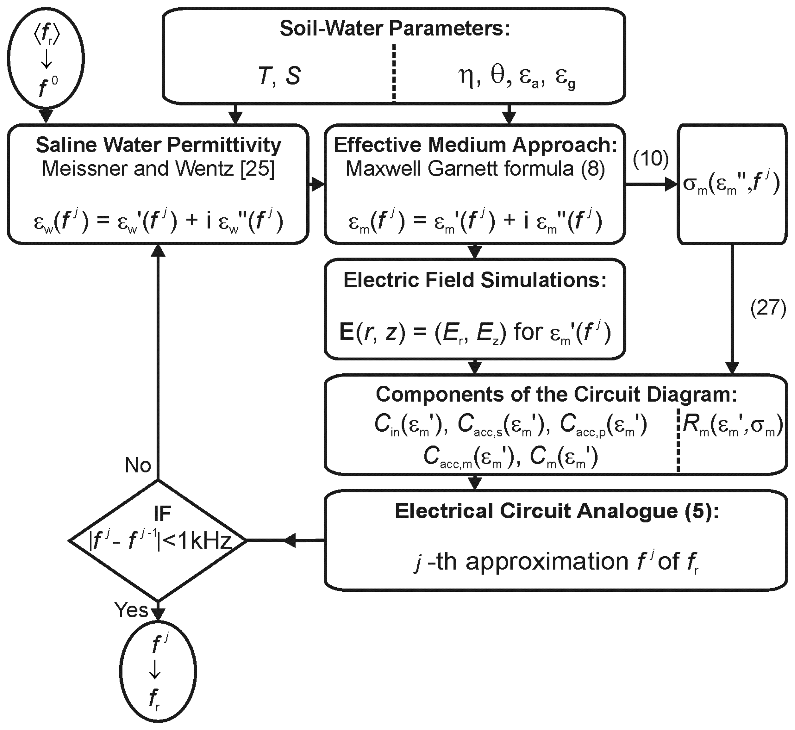
2.5 Iterative Solution Method for the Sensor Resonant Frequency

Because the water permittivity ε_w(f) used in the effective medium approach depends on frequency f, the composite medium is dispersive with ε_m(f) calculated from (8). This implies that the values of the electrical components used for calculating f_r(L, C_p, C_acc,s, C_m, R_m) are not known a priori, because they also depend on f. For this reason the iterative approach sketched in figure 2 involving the models presented above has to be used to compute f_r for a dispersive medium.

The capacitances C_acc,s(ε_m′(f^j)), C_m(ε_m′(f^j)) and C_p(ε_m′(f^j)) = C_in(ε_m′(f^j)) + C_acc,p(ε_m′(f^j)) + C_acc,m used in (5) in the j-th iteration were interpolated from the corresponding capacitances derived from simulated E, and the resistance R_m(ε_m′(f^j), ε_m″(f^j)) was calculated from (10) and (27). The first approximation f¹ is calculated with the circuit diagram elements associated with ε_m(f⁰) corresponding to f⁰ = <f_r> = 130 MHz. Higher-order approximations f^j (j > 1) were calculated from (5) with capacitances and resistor values computed for the permittivity ε_m(f^j-1) at frequency f^j-1. For a broad range of starting frequencies f⁰, this procedure converged within three iterations to an accuracy of |f^j - f^j-1| ≤ 1 kHz yielding the final resonant frequency f_r of the sensor encompassed in a dispersive dielectric medium.

3. Results and Discussion

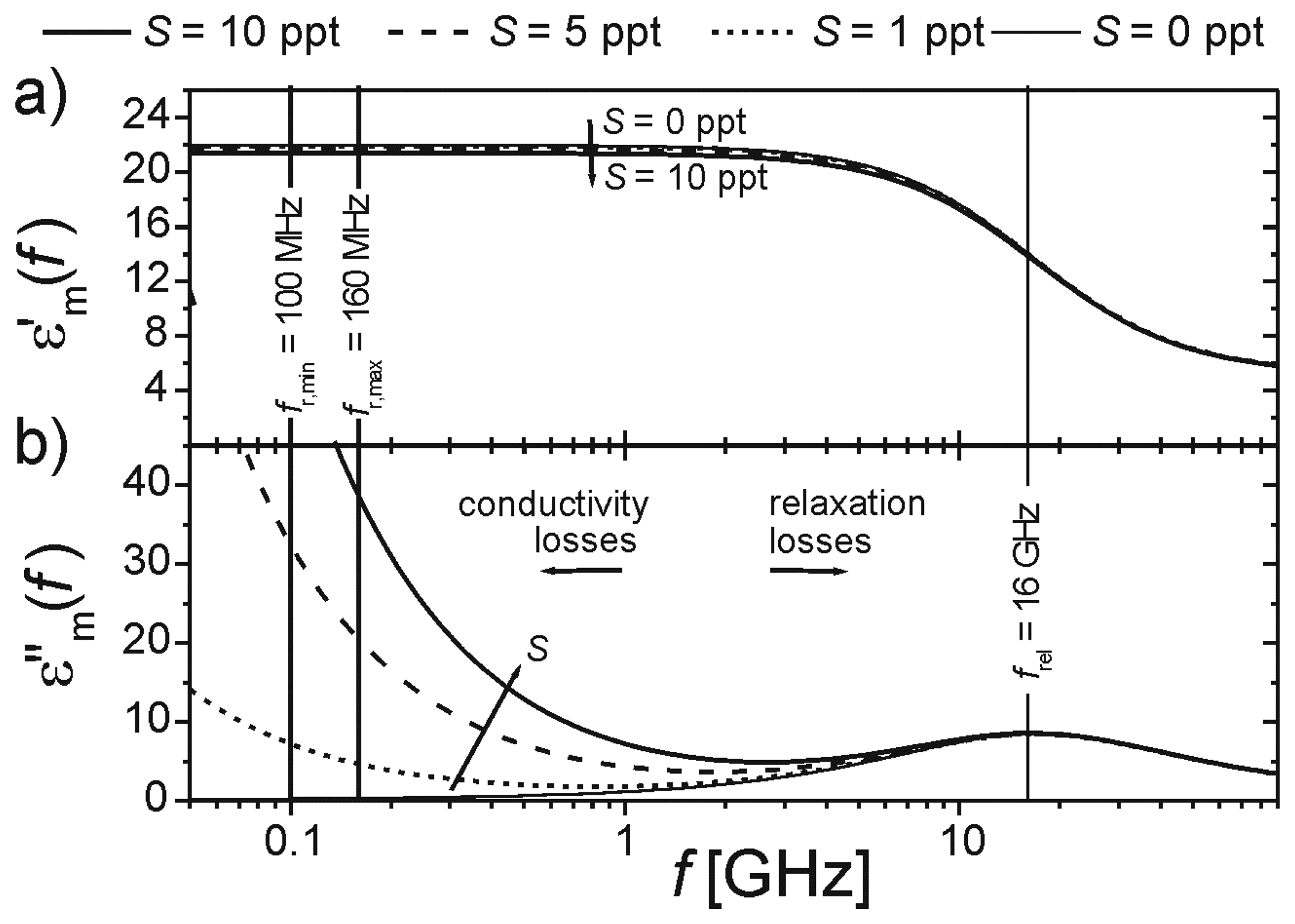
3.1 Frequency-Dependent Permittivity of Porous Media

Figure 5 shows ε_m(f) = ε_m′(f) + i ε_m″(f) computed from the dielectric mixing formula (8). The permittivities ε_g = 5.5 + i 0.2 and ε_a = 1 of the spherical grains and air-bubbles are assumed to be non-dispersive, so the frequency dependence of ε_m(f) is solely due to the dispersive behavior of the water permittivity ε_w(f) = ε_w′(f) + i ε_w″(f) modeled with the approach proposed by Meissner and Wentz [25]. The frequency spectra of the real and the imaginary parts ε_m′(f) and ε_m″(f) were computed for four salinity values S = 0, 1, 5, 10 ppt of the water phase with volumetric content θ= 0.30 m m^-3. The porosity was η=0.4 and the reference temperature T=T_ref=20°C was chosen.

The real part ε_m′(f) decreases slightly with increasing S (figure 5a). Furthermore, the slight slope dε_m′ / df ≈ -5·10^-5 MHz^-1 within the frequency range 100 MHz ≤ f ≤ 1 GHz is almost the same for 0 ppt ≤ S ≤ 10 ppt. The frequency spectra of ε_m″(f) (figure 5b) reveal the relevance of the conductivity losses for f < 1 GHz and of the relaxation losses for higher frequencies. Salinity increases the conductivity contribution to ε_m″(f) but does not affect the contribution due to relaxation. The maximum impact of the relaxation term occurs at f_rel ≈ 16 GHz corresponding to the relaxation frequency of non-saline pure water at T = T_ref = 20°C. The imaginary part ε_m″(f) for S = 0 (thin solid line) includes almost no conductivity contribution. For f = f_rel the gradient dε_m′(f) / df is most distinct as a consequence of the Kramers-Krönig relations [27] relating ε_m′(f) to ε_m″(f).

The resonance frequency band f_r,min ≤ f ≤ f_r,max of the sensor with the boundaries f_r,min = 100 MHz and f_r,max = 160 MHz corresponds with the excited frequencies of the E-field. Therefore, the above spectral analysis of ε_m(f) confirms the assumption made in (10) that ε_m″ is determined solely by σ_m.

Furthermore, the necessity of using an iterative approach to derive f_r becomes obvious by inspecting the variability of θ ε_m″(f). Within the range f_r,min ≤ f ≤ f_r,max, the maximum variation is rather pronounced: ε_m″(f_r,min) - ε_m″(f_r,max) ≈ 23 for S = 10 ppt. Therefore, the value of σ_m calculated from (10) can not be determined if the frequency of the E-field is unknown. By contrast, the maximum difference of the real part is ε_m′(f_r,min) - ε_m′(f_r,max) < 10^-3 for S = 0 ppt, implying that the frequency dependence of ε_m′ does not require f_r to be determined iteratively.

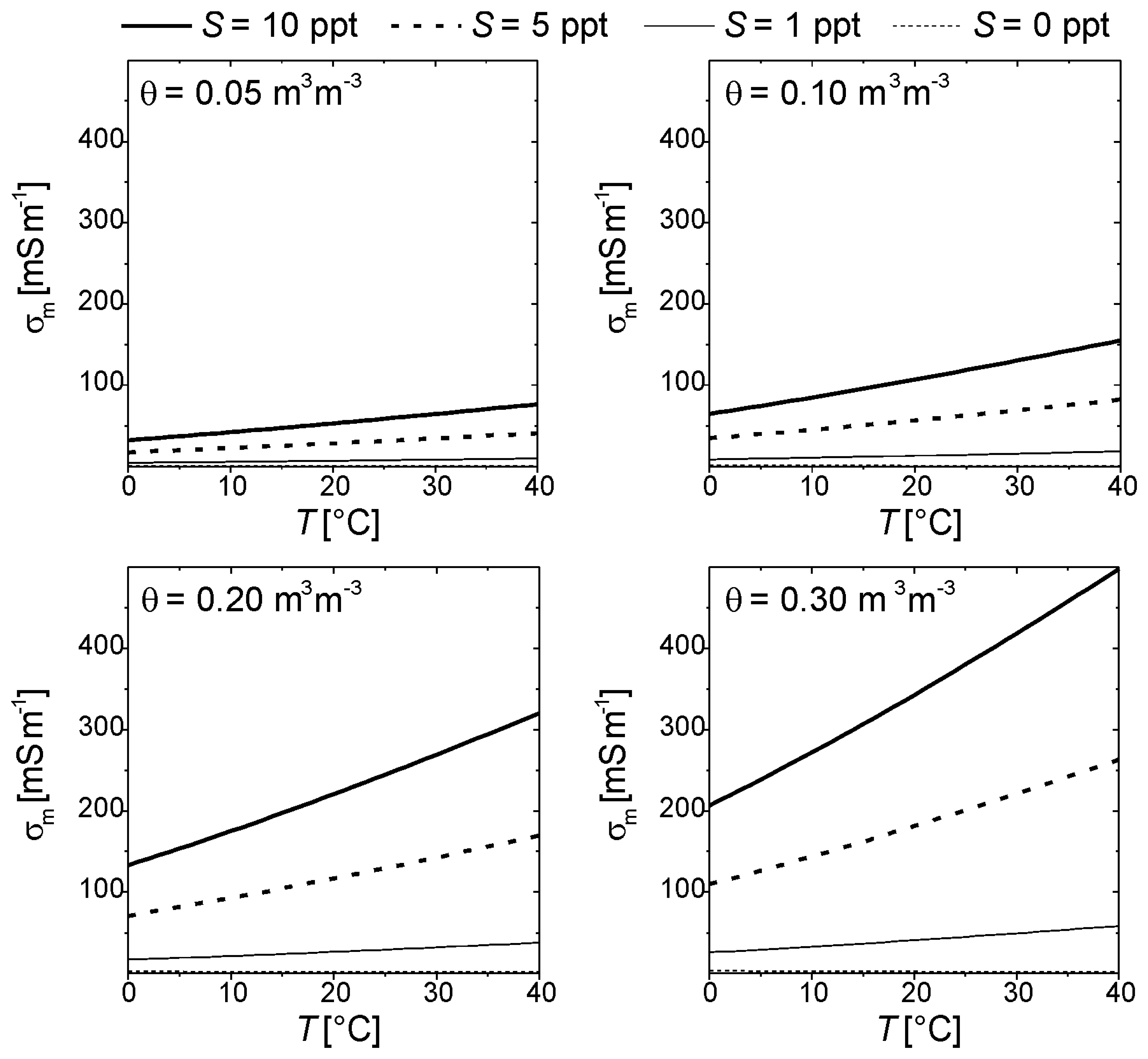
3.2 Temperature Dependencies of Permittivity and Electrical Conductivity

Figure 6 shows temperature dependencies of ε_m′ and ε_m″ computed from (8) for temperatures 0°C ≤ T ≤ 40°C. For this illustration, the frequency of the E-field was set to f = <f_r> = 130 MHz corresponding to an intermediate sensor resonance. The four different line types are results for liquid salinities S = 0, 1, 5, 10 ppt and each of the four bundles of lines in figure 6a (indicated by the ellipses) contains ε_m′(T) computed for the water contents θ = 0.05, 0.10, 0.20, 0.30 m³m^-3. Bound water was ignored here, which may have affected the results at low values of θ.

The real part ε_m′(T) decreases whereas the imaginary part ε_m″(T) increases with increasing T. As expected, increasing θ increases both ε_m′ and ε_m″, and increasing S generally reduces ε_m′ but increases ε_m″ (compare lines for equal θ in figure 6b). The temperature gradients dε_m′/dT are negative and essentially unaffected by S but more distinct for higher q taking values of dε_m″/dT ≈ -0.01 K^-1 for θ = 0.05 m³m^-3 to dε_m′/dT ≈ -0.08 K^-1 for θ = 0.30 m³m^-3. The temperature gradients dε_m″/dT of the imaginary parts are always positive and clearly increase with θ and S. For S = 0 ppt, the values of ε_m″ are close to zero and dε_m″/dT < 0 (thin dashed lines in figure 6b).

The same set of θ and S used in the calculations of ε_m(T) shown in figure 6 were selected for the computation of σ_m(T, θ, S) shown in figure 7. Again, σ_m increases with T for all θ and all S > 0. Values of σ_m ≈ 400 mS m^-1 were modeled for T ≈ 30°C, θ = 0.30 m³m^-3, and S = 10 ppt. Thus, the range of σ_m evaluated here is reasonable for the electrical conductivity of field soils. However, bulk electrical conductivity values of field soils are not necessarily the exclusive result of soil-water salinity. The implied relationship between S and σ_m is limited to “ideal” granular media, but many soils with clay minerals exhibit enhanced electrical conductivity even for non-saline soil water. Nevertheless, the relationship in (10) for σ_m(ε_m″) remains valid.

3.3 Numerical Simulations of Electrical Fields

Figure 8a shows values of circuit diagram capacitances for media permittivities ε_acc = 3.35 ≤ ε_m′ ≤ 80. C_tot(ε_m′) (solid squares) are the measured values of total capacitance; and C_in(ε_m′) values (stars) were derived from (11) using C_out(ε_m′) values (diamonds) computed from the field energy ϕ_out within the volume V_out using the relations (14) and (15). The capacitance of the media C_m(ε_m′) (open circles) and the serial part of the access tube capacitance C_acc,s(ε_m′) (up-triangles) caused by the double-layer of charges at the outer access tube boundary were calculated using the relations (16) - (22), and C_acc,m (dashed line) representing the capacitance due to the volume V_out for ε_m′ = ε_acc = 3.35 was computed as C_acc,m = C_out(ε_m′ = ε_acc) = 3.63 pF. The parallel part C_acc,p(ε_m′) (down-triangles) was computed using (23) and (24).

The values of C_tot, C_in, and C_out increase nonlinearly with ε_m′ taking values of 12.5 pF ≤ C_tot ≤ 26.9 pF and 8.8 pF ≤ C_in ≤ 16.5 pF, and 4.1 pF ≤ C_out ≤ 10.5 pF for 3.35 = ε_acc ≤ ε_m′ ≤ 80. Both C_in(ε_m′) and C_out(ε_m′) increase at similar rates, even though there is no change in permittivity of the inner volume (r ≤ r_acc,in), which indicates that the electrical field inside the capacitor rings is affected by ε_m′ outside the rings and access tube. The values of C_acc,p(ε_m′) < 0.22 pF are clearly small compared with the other parallel capacitances of the circuit diagram (figure 1a) and thus of minor importance for the resonance of the sensor. For ε_m′ approaching ε_acc = 3.35, the values of the two polarization-induced capacitances C_acc,s(ε_m′) and C_m(ε_m′) approach zero, because no double-layer of charges exists at the outer access tube boundary r = r_acc,out.

Values of the geometric factor of the medium g_m(ε_m′) (open circles) were calculated from (28) using the almost linearly increasing C_m(ε_m′) as shown in figure 8b. Unlike previous assumptions that geometric factors are constant for a given sensor [14], we found that g_m(ε_m′) varies substantially and nonlinearly over the permittivity range corresponding to soils from dry to wet conditions. Another geometric factor g_out(ε_m′) (diamonds) associated with C_out(ε_m′) is plotted together with g_m(ε_m′), because g_out(ε_m′) includes the parallel influence of C_acc,m, which together with C_acc,s(ε_m′) and C_m(ε_m′) causes g_out(ε_m′) to decrease with ε_m′. Evett et al. [12] noted that the sensed volumes of capacitance sensors may vary with water content. Furthermore, Paltineanu and Starr [17] tested both axial and radial sensitivities of the sensor to the measurement volume. They observed a small difference in radial distance sensed between measurements in soil at different water contents (θ = 0.124 m³m^-3 and 0.179 m³m^-3), which concurs with measured and simulated results in dielectric liquids [18, Table 4] showing increasing radial distance with ε_m′. These studies offer experimental evidence for the fact that the relative distribution of the field energies within the sensor and within the volume proximate to the sensor changes with water content. The dependency of the computed values of g_m and g_out on ε_m′ corroborates these experimental findings qualitatively, but the quantitative relationship between geometric factors and the measurement volume is unknown.

Figure 8c shows R_m(ε_m′, σ_m) evaluated for σ_m = 5, 20, 100, 500 mS m^-1 and 3.35 ≤ ε_m′ ≤ 80. There is a dramatic decrease of R_m with increasing ε_m′ for ε_m′ < 10 (noting the log scale for R_m) corresponding to low water contents θ and represented by the decreasing g_m(ε_m′) in this range. However, as already mentioned and discussed in the next section, for R_m < 10 Ω and for R_m > 1000 Ω, the effects of the resistor on f_r are asymptotic to no resistance and perfect insulation, respectively.

3.4 Sensor Outputs

All of the analyses above lead to the ability to predict the joint effects of salinity S (a surrogate for bulk electrical conductivity here) and media temperature T on the sensor readings. In this section, we present the predicted resonant frequencies f_r as functions of the electrical resistance R_m and conductivity σ_m, then show the predicted temperature sensitivities for a range of water contents θ and salinities S. The normalized sensor reading N from (1) is the final sensor output used to estimate both ε_m′ and θ in field applications.

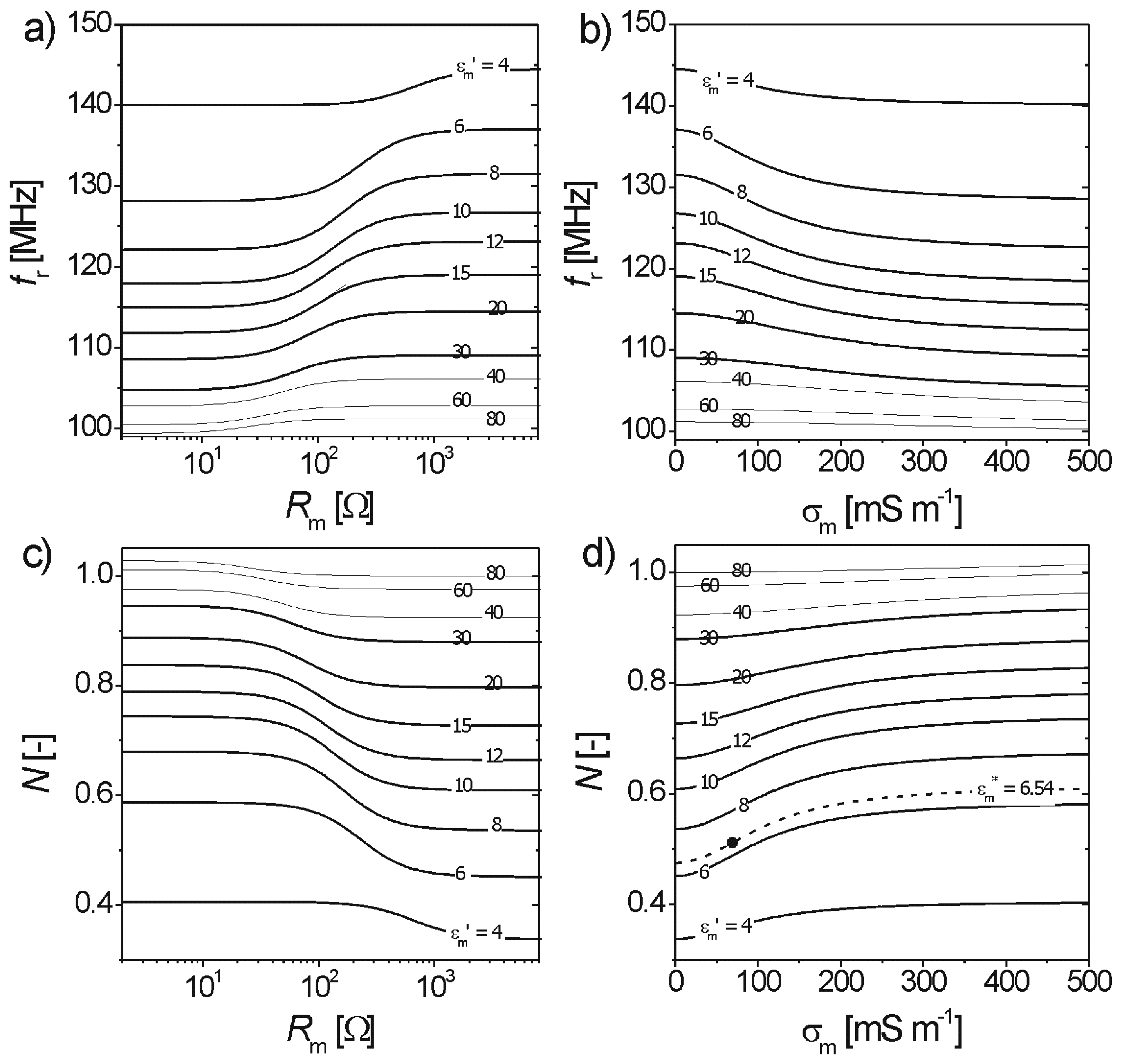
3.4.1 Sensor Resonant Frequency derived from the Circuit Diagram

The sensor resonant frequencies f_r presented below were calculated from (5) representing the resonant frequency of the circuit diagram shown in figure 1. In figure 9a, R_m is considered as an independent variable in the relationship f_r(R_m). The inductance L = 91.95 nH was used as discussed earlier, and the capacitances C_acc,s(ε_m′), C_m(ε_m′), and C_p(ε_m′) used in (5) and computed from the E-field simulated for ε_m′ are listed in

Table 1. Values of capacitances C_acc,s(ε_m′), C_m(ε_m′), and C_p(ε_m′) = C_in(ε_m′) + C_acc,p(ε_m′) + C_acc,m + C_el used in (5) for computing the resonant frequency f_r of the circuit diagram assumed to represent the sensor resonance.

εm′ [-]	Cacc,s [pF]	Cm [pF]	Cp [pF]
4	1.22	0.52	12.83
6	3.38	2.06	13.39
6.54	3.75	2.47	13.51
8	4.50	3.46	13.97
10	5.19	4.93	14.62
12	5.66	6.33	15.18
15	6.13	8.39	15.91
20	6.61	11.84	16.77
30	7.09	18.65	18.03
40	7.34	25.43	18.75
60	7.59	38.98	19.74
80	7.71	52.53	20.19

.

For a realistic range of soil permittivities ε_m′ < 30, the resonant frequencies shown in figure 9a and b (bold lines) are in the range of 104 MHz to 144 MHz and monotonically increasing with decreasing ε_m′. This behavior is in accordance with the increasing resonant frequency of a simple LC-oscillator with decreasing capacitance (compare (6)). Furthermore, for all ε_m′ the computed f_r(R_m) shown in figure 9a takes asymptotically lower values for low R_m and reaches asymptotically higher values for large R_m. This emanates from the circuit diagram (figure 1), revealing that the total capacitance reaches a minimum for R_m → ∞ when C_m(ε_m′) is in series with C_acc,s(ε_m′) and a maximum value for R_m → 0 when C_m(ε_m′) is bypassed. Thus, the resonances of basic LC-oscillators with different operative capacitances (see Equation (6)) qualitatively explains the behavior of f_r(R_m) for low and high values of R_m.

Likewise the dependence f_r(σ_m) shown in figure 9b was calculated from (5). Thereby, R_m(ε_m′, ε_m″) was calculated from C_m(ε_m′) given by (27), and σ_m is considered the free parameter. A corresponding asymptotic behavior is observed for f_r(σ_m). For each ε_m′ the maximum resonance f_r(σ_m = 0) is equal to f_r(R_m → ∞) representing the lossless cases. Likewise, the values of f_r(σ_m = 500 mS m^-1) are almost the same as the corresponding lower-limits f_r(R_m → 0) obtained for a highly lossy medium. The fact that the difference f_r(σ_m = 0) - f_r(σ_m = 500 mS m^-1) is very similar to the difference f_r(R_m → ∞) - f_r(R_m → 0) for any ε_m′ shows that the range 0 ≤ σ_m ≤ 500 mS m^-1 yields values of R_m (see also figure 8c) covering the sensitive range of approximately 10 Ω < R_m < 1000 Ω. This theoretical sensitivity of f_r to R_m coincides with observations of other investigators [3] that f_r may be sensitive to bulk electrical conductivity in the range 0 ≤ σ_m ≤ 500 mS m^-1.

Normalized readings N(R_m) and N(σ_m) calculated from f_r(R_m) and f_r(σ_m) using (1) are shown in figure 9c and d, respectively. Thereby the reference resonant frequencies f_r,k (k = a, w) are associated with a lossless environmental medium (R_m = ∞, σ_m = 0) and thus simply calculated using Equation (6) with L = 91.95 nH, and the operative capacitances C = C_tot,a = 9.93 pF and C = C_tot,w = 26.92 pF for air and pure water at the reference temperature T_ref = 20°C. These values are in agreement with the measured total capacitances presented in Schwank et al. [18] and corrected for the presence of the FEP shrink fit. The resulting reference resonant frequencies are f_r,a = 166.6 MHz and f_r,w = 101.2 MHz, respectively. By virtue of definition (1), dN/dR_m and dN/dσ_m vary in the opposite directions of those for the corresponding df_r/dR_m and df_r/dσ_m.

Based on the simulated sensor responses to changes in electrical conductivity shown in figure 9, we do not expect the predicted response to salinity in water (ε_w′ = 80) to be very large. A simple experimental check of the model response to salinity is given in figure 10, which shows N(S) for water at T = T_ref = 20°C measured in the laboratory (symbols) and simulated (line). The simulated magnitude of response underestimated the measured response, but the shape of the curve, particularly the salinity at which N plateaus, matches the data well. Further experiments in an unsaturated porous medium would be needed to test the model response at lower bulk permittivities, where the sensor response to electrical conductivity is expected to be much greater (figure 9). Such model validation experiments are beyond the scope of the present study.

Permittivities ε̂ (N) derived from sensor outputs N are the proxy-quantities used to infer soil water contents θ in field applications. Soil permittivities ε̂imeasured with the capacitance sensor are predicted to deviate from the value of ε_m′ as the result of electrical conductance σ_m occurring in natural moist soils. The sensitivity dε̂ /dσ_m of the measured proxy ε̂ with respect to σ_m is explored below. Thereby, dε̂ / dσ_m is expressed as:

$$\frac{d\widehat{\epsilon }}{d{\sigma }_{\text{m}}}\left({{\epsilon }^{\prime }}_{\text{m}},{\sigma }_{\text{m}}\right)={\frac{\partial \widehat{\epsilon }}{\partial N}|}_{N\left({{\epsilon }^{\prime }}_{\text{m}},{\sigma }_{\text{m}}\right)}\cdot {\frac{\partial N}{\partial {\sigma }_{\text{m}}}|}_{{{\epsilon }^{\prime }}_{\text{m}},{\sigma }_{\text{m}}}$$

(29)

The partial derivative ∂ε̂ / ∂N is calculated from the empirical relationship ε̂(N) given by (2). The normalized reading N(ε_m′, σ_m) and the corresponding derivative ∂N/∂σ_m evaluated at (ε_m′, σ_m) are computed from the modeled data shown in figure 9d.

The values of dε̂/dσ_m plotted in figure 11a are all positive showing that ε̂ in a conductive medium is always an overestimation of the value ε_m′, which would be measured for σ_m = 0. The distortion of a measurement within the realistic range ε_m′ < 30 (bold lines in figure 11a) is predicted to increase with ε_m′. For 30 < ε_m′ < 80 (thin lines in figure 11a) the gradients dε̂ / dσ_m decrease with increasing ε_m′ because ∂N/∂σ_m becomes very small for high ε_m′ (see figure 9d). However, as a consequence of the distinct nonlinearity of ε̂(N) given by (2), the maximum values of dε̂ / dσ_m do not occur at ε_m′ = 6.54 and σ_m= 69.3 mS m^-1 where the derivative ∂N/∂σ_m = 0.81·10^-3 mS m^-1 is greatest (bold dot on the dashed line in figure 9d).

Simulated relative changes δε̂ = Δε̂ / ε_m′ of permittivities ε̂ measured with the capacitance sensor in conductive media are plotted in figure 11b. Wherein, the absolute change Δε̂ is defined as the difference between the simulated value in a non-conducting medium (σ_m = 0) and corresponding simulations for σ_m > 0 at the same water content θ. The difference Δε̂(ε_m′, σ_m) can be expressed using (29) as:

$$\mathrm{\Delta }\widehat{\epsilon }\left({{\epsilon }^{\prime }}_{\text{m}},{\sigma }_{\text{m}}\right)=\underset{0}{\overset{{\sigma }_{\text{m}}}{\int }}d\widehat{\epsilon }=\underset{0}{\overset{{\sigma }_{\text{m}}}{\int }}\frac{d\widehat{\epsilon }}{d{\sigma }_{\text{m}}}\left({{\epsilon }^{\prime }}_{\text{m}},{\sigma }_{\text{m}}\right)\cdot d{\sigma }_{\text{m}}$$

(30)

The calculations reveal rather large positive values of δε̂ for σ_m > 50 mS m. This clearly shows that permittivities of electrically conducting media (soils) are expected to be overestimated if measured with a capacitance sensor. Other investigators [28, 29] reported salinity effects on capacitance sensors continuing at high bulk electrical conductivities (i.e., σ_m > 500 mS m^-1), which may not contradict the present model at relatively high soil water contents and associated permittivities (e.g., ε_m′ > 30). However, we do not expect σ_m to affect the sensor readings much at low θ and σ_m > 500 mS m^-1.

In practice the simulated δε̂ can be used to compensate for the enhancing effect of σ_m on ε̂(N) measured in a conductive medium. The resulting real part ε_m′ of the soil permittivity, which would be measured for σ_m = 0, is the proxy-quantity used to infer the soil water content θ. Thus, one can compute permittivity ε_m′ corrected for electrical conductivity using such a correction function:

$${{\epsilon }^{\prime }}_{\text{m}}\left(\widehat{\epsilon },{\sigma }_{\text{m}}\right)=\widehat{\epsilon }\cdot \left(1-\delta \widehat{\epsilon }\left(\widehat{\epsilon },{\sigma }_{\text{m}}\right)\right)$$

(31)

In this equation, temperature affects permittivity via its effect on electrical conductivity, but the direct effect of temperature on water permittivity is not included as it is not a sensor effect.

3.4.2 Temperature Dependence of Resonant Frequency and Normalized Reading

The temperature dependence of f_r(T) is caused primarily by the temperature sensitivity of the imaginary part of the medium permittivity ε_m″(T). As ε_m(f) and especially ε_m″(f) are frequency dependent, the resonance f_r must be calculated iteratively following the procedure illustrated in figure 2.

Figure 12a shows f_r(T) calculated for the porosity η = 0.4, grain permittivity ε_g = 5.5 + i 0.2, and for a set of salinities S = 0, 1, 5, 10 ppt and water contents θ = 0.05, 0.10, 0.20, 0.30 m³ m^-3. The corresponding predicted resonant frequencies are in the range of 109 MHz ≤ f_r ≤ 136 MHz. This is approximately the same as the range from f_r(R_m → ∞) to f_r(σ_m = 0) calculated for 6 ≤ ε_m′ ≤ 30 (figure 9) representing a reasonable permittivity range for soil-water conditions.

Depending on S and θ, positive or negative temperature responses f_r(T)/dT were predicted. For low S, values of ε_m″ are low, leading to values of R_m which exceed the upper limit of the sensitivity range (≈ 1000 Ω) affecting f_r. Under these circumstances, f_r values are determined predominantly by the total capacitance C_tot(ε_m′) which increases with ε_m′ (figure 8a). Therefore, the negative temperature gradient dε_w′/dT ≈ -0.36 K^-1 [25] leads to the predicted positive frequency responses f_r(T)/dT > 0 for low S. Observations in real soils [3, 29] displayed f_r/dT < 0 even for nonsaline soil water due to σ_m > 0 associated with charged particles. This difference points out a limitation of the simplified model, such that one needs to consider σ_m rather than merely S in real soils.

As S increases to 10 ppt, df_r(T)/ dT decreases and becomes negative, particularly for the intermediate water contents 0.10 m³ m^-3 ≤ θ ≤ 0.20 m³ m^-3. This behavior is in accordance with increasing losses leading to R_m within the sensitive range (10 Ω < R_m < 1000 Ω) affecting f_r. Consequently, the gradients df_r(T)/dT are affected by dσ_m/dT which reaches highly positive values for large S (see figure 7) leading to dR_m/dT < 0 (not shown here). The negative temperature coefficients dR_m/dT < 0 explain the negative gradients df_r(T)/dT predicted for high S, because f_r decreases with decreasing R_m (figure 9a). Normalized readings N(T) shown in figure 12b were computed from f_r(T) using (1) with f_r,a = 166.6 MHz and f_r,w = 101.2 MHz respectively. As a result, dN/dT varies in the opposite directions of those for the corresponding df_r/dT.

Finally, we estimated ε̂(T) (the apparent, measured permittivity in a conducting soil medium) from the empirical relationship (2) for comparison with the value ε_m′ of the real part of the medium permittivity computed directly from the mixing model (figure 6). Figure 13 shows temperature dependencies of relative deviations δε̂ = Δε̂/ε_m′ simulated for θ = 0.05, 0.10, 0.20 0.30 m³ m^-3 , S = 0, 1, 5, 10 ppt and for ε_g = 5.5 + i 0.2, η = 0.4. In the following, Δε̂ is defined as the difference between simulated values ε̂ expected to be derived from the sensor reading N at the reference temperature T = T_ref = 20°C and the corresponding simulation for T ≠ T_ref. As an extension to (30) Δε̂(S, θ, T) is expressed as:

$$\mathrm{\Delta }\widehat{\epsilon }\left(S,\theta ,T\right)=\underset{T_{\text{ref}}}{\overset{T}{\int }}d\widehat{\epsilon }=\underset{T_{\text{ref}}}{\overset{T}{\int }}\frac{d\widehat{\epsilon }}{dT}\left(S,\theta ,T\right)\cdot dT$$

(32)

Thereby, the temperature sensitivity of the proxy value ε̂ used to infer the soil moisture is expressed as:

$$\frac{d\widehat{\epsilon }}{dT}\left(S,\theta ,T\right)={\frac{\partial \widehat{\epsilon }}{\partial N}|}_{N\left(S,\theta ,T\right)}\cdot {\frac{\partial N}{\partial T}|}_{S,\theta ,T}$$

(33)

Again, ∂ε̂/∂N evaluated at N(S, θ, T) was derived from (2), and ∂N/∂T evaluated at (S, θ, T) was computed from the simulated values of N(S, θ, T) shown in figure 12b.

The real part of the medium permittivity ε_m′ used to estimate the relative deviation δε̂ = Δε̂/ε_m′ is computed from the dielectric mixing model (8) evaluated for T = T_ref = 20°C, S = 0 ppt and f = <f_r> = 130 MHz. The frequency-dependence of these ε_m′ for 0 ppt ≤ S≤ 10 ppt and for f within the resonant frequency band f_r,min ≤ f≤ f_r,_max is minor (see figure 5), so the choice of f is not critical.

The resulting values computed for the four water contents θ are indicated in the corresponding panels of figure 13. For increasing T > T_ref and for S = 0 (thin dashed lines in figure 13) computed δε̂ are increasingly negative. As σ_m is almost zero in this case for all T (see figure 7), the difference Δε̂ between the simulated ε̂ for T ≠ T_ref and for T = T_ref is not caused by the effect of the medium conductivity on the sensor output N (see figure 9).

Consequently, the relative deviations δε̂ for S = 0 are associated with the decrease of the real part of the permittivity ε_m′ with increasing T in accordance with the negative temperature coefficient dε_w′/dT ≈ -0.36 K^-1 [25] of the liquid phase with volumetric content θ. Computed δε̂ for S = 1 ppt (thin solid lines) are less negative for T > T_ref because the sensor output N increases with σ_m as a function of T (see figure 7), which partially compensates for the negative gradients dε_m′/dT (see figure 6a). For S = 5 ppt and 10 ppt (bold dashed and solid lines) the even higher values of σ_m with T (see figure 7) cause N to increase with T such that δε̂ becomes greater than zero for T > T_ref meaning that the negative gradients dε_m′/dT of the real parts of the medium permittivities are dominated by conductivity effects. However, for S = 10 ppt and θ = 0.30 m³ m^-3 the correspondingly high values σ_m exceed the sensitive range of N (figure 9) such that the negative temperature gradient dε_m′/dT has a dominant effect on ε̂ deduced from N simulated for T > 20°C. At lower water contents (e.g., θ = 0.10 m³ m^-3), the positive effect of T on δε̂ is nearly linear for S = 10 ppt over the whole temperature range.

4. Summary and Conclusions

The capacitance sensor investigated here is used to infer soil water content θ either from a direct empirical relationship between θ and measured resonant frequency f_r (after normalization by air and water counts) or via estimation of the real part of permittivity ε_m′ as a proxy for θ(ε_m′). Here, we refined the theoretical understanding and quantification of the sensor responses to variable θ, temperature T, and liquid salinity S, including resulting changes in the bulk electrical conductivity of granular soils σ_m. This was achieved by combining a dielectric mixing model, electrical circuit analogue, and finite-element numerical model of the electrical field in and around the sensor for a range of environmental conditions. Within the mixing model, the complex permittivity of saline water was based on previous empirical studies [24]. The model does not handle bulk electrical conductivity due to charged clays, but liquid salinity provides analogous dielectric conditions in the combined model. Effects of bound water on em were not considered here, but are left for future investigations using a more sophisticated mixing model.

The frequency dependence of ε_m is confirmed and quantified by the mixing model, showing that ε_m′ is relatively insensitive to S, while ε_m″ can be highly sensitive to both S and f at a given water content and temperature (see figure 5). In the measured frequency range of the sensor (100 < f_r < 160 MHz), this sensitivity is due to conductivity losses rather than high-frequency relaxation losses. The computed values of ε_m′(θ, S, T) decrease with T for all values of θ and S, while the imaginary part ε_m″(θ, S, T) increases with T, and the slope dε_m″/dT increases with both θ and S. Again, S may be considered as surrogate for bulk electrical conductivity, σ_m, given knowledge of the multivariate response of σ_m(θ, S, T). Monotonic increases in σ_m with θ, S, and T were estimated (figure 7) and used to compute bulk electrical resistance R_m in the electrical circuit analogue. R_m(ε_m′) was shown to be highly sensitive to ε_m′ only for ε_m′ < 10 (figure 8c).

In addition to R_m, various components of the total sensor capacitance as functions of ε_m′ were computed from numerical simulations of the electrical field, where C_m(ε_m′) was found to be nearly linear (figure 8a). However, the associated geometric factor g_m(ε_m′) of the medium of interest was shown to be highly variable (0 < g_m < 0.75) and nonlinear for ε_m′ < 25 (figure 8b). This indicates that the geometry of the electrical field surrounding the ring capacitor changes with the permittivity of the medium being measured, as indicated in previous experiments [12, 17, 18].

Given all circuit component values as functions of the environmental variables (θ, S, and T), the resonant frequency and its normalized value N were computed as functions of R_m or σ_m. Values of N increased with σ_m for all values of ε_m′(θ), with a maximum sensitivity at ε_m′ = 6.54 (figure 9). Thus, the apparent permittivity ε̂(N) and water content θ(N) are sensitive to σ_m. Estimation errors for ε_m′ were computed as functions of σ_m and T using the combined model. Temperature variations in the range 0 < T < 40°C caused deviations in ε̂_m′ within a range of almost ± 10 % (figure 13). No additional temperature drifts of the sensor electronics were considered here.

The physics-based theory presented here is of general validity for understanding the sensitivity of capacitance sensors to the electrical conductivity of the surrounding media. Because the soil electrical conductivity also depends on temperature, the resulting modeled instrumental sensitivity has to be taken into account before interpreting thermal effects in measured data. Future studies may use the present approach and results to identify functions to correct for temperature and salinity effects on the estimated soil water content. Such correction functions can then be compared with laboratory and field data. Based on the potential errors in frequency-based estimates of permittivity computed here, field data measured with such capacitance sensors will not provide reliable absolute estimates of water content without such correction functions.

References

1. Fares, A.; Hamdhani, H.; Jenkins, D.M. Temperature-Dependent Scaled Frequency: Improved Accuracy of Multisensor Capacitance Probes. Soil Sci. Soc. Am. J. 2007, 71(3). accepted for publication. [Google Scholar]
2. Bakhtina, E.Y.; Il'in, V.A. Investigation of dielectric properties of sand at cryogenic temperatures. Journal of Communications Technology and Electronics 1999, 44(8), 939–941. [Google Scholar]
3. Baumhardt, R.L.; Lascano, R.J.; Evett, S.R. Soil material, temperature, and salinity effects on calibration of multisensor capacitance probes. Soil Sci. Soc. Am. J. 2000, 64(6), 1940–1946. [Google Scholar]
4. Jones, S.B.; Or, D. Surface area, geometrical and configurational effects on permittivity of porous media. Journal of Non-Crystalline Solids 2002, 305(1-3), 247–254. [Google Scholar]
5. Logsdon, S.; Laird, D. Cation and water content effects on dipole rotation activation energy of smectites. Soil Sci. Soc. Am. J. 2004, 68(5), 1586–1591. [Google Scholar]
6. Seyfried, M.S.; Murdock, M.D. Response of a new soil water sensor to variable soil, water content, and temperature. Soil Sci. Soc. Am. J. 2001, 65(1), 28–34. [Google Scholar]
7. Seyfried, M.S.; Murdock, M.D. Measurement of soil water content with a 50-MHz soil dielectric sensor. Soil Sci. Soc. Am. J. 2004, 68(2), 394–403. [Google Scholar]
8. Wraith, J.M.; Or, D. Temperature effects on soil bulk dielectric permittivity measured by time domain reflectometry: Experimental evidence and hypothesis development. Water Resources Research 1999, 35(2), 361–369. [Google Scholar]
9. Blonquist, J.M., Jr.; Jones, S.B.; Robinson, D.A. Standardizing Characterization of Electromagnetic Water Content Sensors: Part 2. Evaluation of Seven Sensing Systems. Vadose Zone J. 2005, 4(4), 1059–1069. [Google Scholar]
10. Jones, S.B.; Blonquist, J. M., Jr.; Robinson, D. A.; Rasmussen, V. P.; Or, D. Standardizing Characterization of Electromagnetic Water Content Sensors: Part 1. Methodology. Vadose Zone J. 2005, 4(4), 1048–1058. [Google Scholar]
11. Gong, Y.; Cao, Q.; Sun, Z. The effects of soil bulk density, clay content and temperature on soil water content measurement using time-domain reflectometry. Hydrological Processes 2003, 17(18), 3601–6314. [Google Scholar]
12. Evett, S.R.; Tolk, J.A.; Howell, T.A. Soil Profile Water Content Determination: Sensor Accuracy, Axial Response, Calibration, Temperature Dependence, and Precision. Vadose Zone J. 2006, 5(3), 894–907. [Google Scholar]
13. Or, D.; Wraith, J.M. Temperature effects on soil bulk dielectric permittivity measured by time domain reflectometry: A physical model. Water Resources Research 1999, 35(2), 371–383. [Google Scholar]
14. Kelleners, T.J.; Soppe, R.W.O.; Robinson, D.A.; Schaap, M.G.; Ayars, J.E.; Skaggs, T.H. Calibration of capacitance probe sensors using electric circuit theory. Soil Sci. Soc. Am. J. 2004, 68(2), 430–439. [Google Scholar]
15. Robinson, D.A.; Kelleners, T.J.; Cooper, J.D.; Gardner, C.M.K.; Wilson, P.; Lebron, I.; Logsdon, S. Evaluation of a Capacitance Probe Frequency Response Model Accounting for Bulk Electrical Conductivity: Comparison with TDR and Network Analyzer Measurements. Vadose Zone J. 2005, 4(4), 992–1003. [Google Scholar]
16. Robinson, D.A.; Jones, S.B.; Wraith, J.M.; Or, D.; Friedman, S.P. A Review of Advances in Dielectric and Electrical Conductivity Measurement in Soils Using Time Domain Reflectometry. Vadose Zone J. 2003, 2(4), 444–475. [Google Scholar]
17. Paltineanu, I.C.; Starr, J.L. Real-time soil water dynamics using multisensor capacitance probes: Laboratory calibration. Soil Sci. Soc. Am. J. 1997, 61, 1576–1585. [Google Scholar]
18. Schwank, M.; Green, T.R.; Mätzler, C.; Benedickter, H.; Flühler, H. Laboratory Characterization of a Commercial Capacitance Sensor for Estimating Permittivity and Inferring Soil Water Content. Vadose Zone J. 2006, 5(3), 1048–1064. [Google Scholar]
19. Starr, J.L.; Timlin, D.J. Using High-Resolution Soil Moisture Data to Assess Soil Water Dynamics in the Vadose Zone. Vadose Zone J. 2004, 3(3), 926–935. [Google Scholar]
20. Terman, F.E. Radio engineers' handbook.Vol., 1st ed.; 6th impr; 1943; New York; McGraw-Hill; p. 1019. [Google Scholar]
21. Sihvola, A. Electromagnetic mixing formulas and applications.; Electromagnetic Waves Series 47; 1999; London; The Institution of Electrical Engineers. [Google Scholar]
22. Maxwell Garnett, J.C. Colours in metal glasses and metal films. Trans. Royal Society (London) 1904, CCIII, 197–202. [Google Scholar]
23. Santamarina, J.C.; Klein, K.A.; Fam, M.A. Soils and Wave.; 2001; Hoboken; NJ John Wiley & Sons. [Google Scholar]
24. Mätzler, C. in Minerals and rocks; Thermal Microwave Radiation-Applications for Remote Sensing; 2006; London, UK. [Google Scholar]
25. Meissner, T.; Wentz, F.J. The complex dielectric constant of pure and sea water from microwave satellite observations. IEEE Trans. Geosci. Remote Sensing 2004, 42(9), 1836–1849. [Google Scholar]
26. Haus, H.A.; Melcher, J.R. Electromagnetic Fields and Energy. 1998. available from: http://web.mit.edu/6.013_book/www/ [cited 11 Oct. 2006].
27. Jackson, J.D. Classical Electrodynamics., Third ed.; 1999; Wiley, cop., 1999; p. 808.
28. Kelleners, T.J.; Soppe, R.W.O.; Ayars, J.E.; Skaggs, T.H. Calibration of capacitance probe sensors in a saline silty clay soil. Soil Sci. Soc. Am. J. 2004, 68, 770–778. [Google Scholar]
29. Evett, S.R.; Lauerent, J.P.; Cepuder, P.; Hignett, C. Neutron scattering, capacitance, and TDR soil water content measurements compared on four continents. Proc. 17th World Congress Soil. Sci., Thailand, 14-21 Aug. 2002; pp. 1021-1–1021-10.
Figure 1. Circuit diagram used for modeling the frequency response of the capacitance sensor (a and b).Total capacitance is composed of Cin and Cout due to volume inside and outside the inner access tube boundary. Cacc,p and Cacc,s are the parallel and the serial parts of the access tube capacitance, respectively. Cacc,m accounts for the capacitance of the volume outside the inner access tube boundary if the dielectric contrast between the medium and the access tube disappears. The parallel connection of Cm and Rm is the electrical analogue of the conductive medium (soil) outside the access tube. The symbolic justification of Cacc,m is sketched in panel c.
Sensors 07 00548f1
Figure 2. Flow-chart of the iterative approach for modeling the sensor resonance fr determined by the sensor properties (figure 1) and the effective permittivity εm of the porous solid-water-air medium (soil) surrounding the probe. Relevant equation numbers are indicated (in parentheses).
Sensors 07 00548f2
Figure 3. a) Sensor with symbolized electric field E. b) Sketch of the cross section of the sensor considering the rotational symmetry with respect to the z-axis and the mirror symmetry with respect to the plane perpendicular to z in the middle of the two ring electrodes (z = 0). This geometry is used for simulating the electric field E caused by a potential difference between the ring electrodes (1 inch = 25.4 mm).
Sensors 07 00548f3
Figure 4. Schematic diagram of the structure of the porous medium used for modeling the effective medium permittivity εm representing the moist soil surrounding the sensor access tube. The grains with permittivity εg and the air-bubbles with permittivity εa are approximated by spherical inclusions in water with permittivity εw.
Sensors 07 00548f4
Figure 5. Frequency spectrum of εm(f) = εm′(f) + i εm″(f) for a set of liquid salinities S = 0, 1, 5, 10 ppt calculated for: η = 0.4, εg = 5.5 + i 0.2, T = Tref = 20°C, θ = 0.3 m3m-3. The frequencies fr,min and fr,max are the boundaries of the resonance frequency band of the sensor.
Sensors 07 00548f5
Figure 6. a) Computed real parts εm′(T) and b) imaginary parts εm″(T) of the porous two-phase mixture (η = 0.4) comprising spherical grains (εg = 5.5 + i 0.2) and air-bubbles (εa = 1) embedded in water, computed for S = 0, 1, 5, 10 ppt and θ = 0.05, 0.10, 0.20, 0.30 m3m-3.
Sensors 07 00548f6
Figure 7. Calculated electrical conductivities σm(T) of the porous multiphase medium assumed to be representative for the wet soil. The same set of values for θ and S are chosen as for the results shown in figure 6.
Sensors 07 00548f7
Figure 8. Capacitances used in the circuit analogue for computing sensor resonance fr. Ctot was based on measurements, Cin, Cout, Cacc,p, Cacc,s, and Cm were calculated from the E-field modeled for 3.35 = εaccεm′ ≤ 80, and Cacc,m = 3.63 pF represents the capacitance for εm′ = εacc of the volume Vout. b) Geometric factors gm and gout derived from Cm and Cout. c) Resistance Rm of the medium derived from Cm using (27) for four different conductivities σm = 5, 20, 100, 500 mS m-1.
Sensors 07 00548f8
Figure 9. a) Resonance frequencies fr versus resistance Rm of the medium and b) fr versus medium conductivity σm. c) Normalized sensor reading N versus Rm and d) N versus σm.
Sensors 07 00548f9
Figure 10. Measured (symbols) and simulated (line) values of normalized sensor reading N(S) for saline water surrounding the sensor. Electrical conductivity σw of water with salinity S is computed for the experimental conditions (T = Tref = 20°C).
Sensors 07 00548f10
Figure 11. a) Gradients dε̂ / m representing the sensitivities of measured permittivities ε̂ (N) with respect to electrical medium conductivity σm. b) Simulated relative overestimations δε̂ = Δε̂ / εm′ of measurements taken in conductive media.
Sensors 07 00548f11
Figure 12. a) Computed resonant frequencies fr(T) and b) corresponding normalized readings N(T) of the capacitance sensor. The calculations were based on the electrical properties εm(T) and σm(T) of the environmental porous medium shown in figure 6 and 7, respectively. Furthermore, the electrical circuit analogue evaluated for the partial capacitances derived from the field simulations were used to calculate fr.
Sensors 07 00548f12
Figure 13. Relative deviations δε̂ = Δε̂/ εm′ between simulated ε̂ for T = Tref = 20°C and TTref. The value εm′ is computed from (8) with S = 0 ppt, Tref = 20°C, f = 130 MHz, εg = 5.5 + i 0.2, and η = 0.4.
Sensors 07 00548f13